Experimental entanglement distillation using Schmidt projection on multiple qubits

Abstract

Entanglement distillation is a procedure for extracting from one or more pairs of entangled qubits a smaller number of pairs with a higher degree of entanglement that is essential for many applications in quantum information science. Schmidt projection is a unique distillation method that can be applied to more than two pairs of entangled qubits at the same time with high efficiency. We implement the Schmidt projection protocol by applying single-photon two-qubit quantum logic to a partially hyperentangled four-qubit input state. The basic elements of the procedure are characterized and we confirm that the output of Schmidt projection is always maximally entangled independent of the input entanglement quality and that the measured distillation efficiency agrees with theoretical predictions. We show that our implementation strategy can be applied to other quantum systems such as trapped atoms and trapped ions.

I INTRODUCTION

Shared entanglement is an essential resource in many quantum information processing applications such as quantum teleportation Teleportation , quantum computation KLM ; QTeleportationComputing ; OneWayQComputer , quantum cryptography QKDEntanglement , and quantum repeaters QRepeater . These applications generally require that two remote parties maintain a very high degree of entanglement in order for their protocols to work properly. Therefore, the generation of maximally entangled states such as the Bell states is an essential task in quantum information science. However, even if one can initially generate maximally entangled states with ease, they often become non-maximally entangled or partially mixed at the remote locations because of dissipation and decoherence through interactions with the environment. While each application has its own level of tolerance to entanglement degradation, most applications would be practically unusable without some kind of procedure to restore the degraded entanglement to its initial maximally entangled state.

The need for most quantum information processing applications to overcome unavoidable loss of entanglement has led to several methods for entanglement restoration Concentration ; PurificationCNOT ; PurificationParity1 ; LocalFiltering ; NoPostSelection ; Procrustean ; PurificationParity2 ; Parity1 ; Parity2 . These techniques typically seek to improve the quality of entanglement between a pair of entangled qubits by selecting, filtering, and applying unique processing algorithms to a larger number of lower quality entangled qubits. Entanglement restoration provides a path to utilizing entangled qubits that would otherwise be dicarded because their entanglement quality is below the threshold necessary for specific applications. The cost of entanglement restoration is that many pairs of the lower quality entangled qubits must be generated and processed, which requires more resources and longer times for each application processing step. It is therefore of interest to choose a method that is efficient in terms of resources and processing required to achieve a certain level of entanglement quality. Among these methods, Schmidt projection (SP) Concentration has the interesting property that it can be applied to more than two pairs of entangled qubits at the same time and that the distillation efficiency can approach unity when applied to a large number of initial pairs. Despite these advantages, Schmidt projection is considered difficult to implement because it requires simultaneous collective measurements on multiple qubits.

In this work, we illustrate the working principle of Schmidt projection Concentration by applying the technique to two pairs of partially entangled qubits. First, we use the concept of physical mapping to encode the two pairs of entangled qubits into four physically distinguishable states of two hyperentangled photons. The two photons are entangled in both polarization and momentum degrees of freedom so that the four qubits can be distinguished by their photon, polarization, and momentum. By hosting two qubits per photon carrier, we eliminate the problem of bringing the two qubits together to overlap completely in time for quantum logic gate operations. Moreover, the two types of qubits can be manipulated deterministically using single-photon two-qubit (SPTQ) quantum logic PCNOT ; SPTQSWAP . The SP protocol is carried out efficiently using SPTQ quantum gates to produce a single maximally-entangled pair of qubits. In Sect. II we describe the basic idea of the SP protocol and show how this protocol can be implemented with hyperentangled photon pairs. Section III describes our experimental implementation including the generation of partially hyperentangled photons and the use of SPTQ logic to perform the Schmidt projection. The resulting maximally polarization-entangled photons are characterized and the effectiveness and efficiency of the protocol are analyzed and discussed in Sect. IV, and finally we summarize and show how the concept of physical mapping can be applied to trapped-atom and trapped-ion systems.

II THEORETICAL BACKGROUND

Before we describe how the Schmidt projection protocol can be implemented in our experiment, it is useful to clarify the sometimes confusing terminology in entanglement restoration. Given one or more pairs of entangled qubits one can extract from them a smaller number of pairs with a higher degree of entanglement (or the same number of pairs with less than unity probability) by using local operations and classical communication. This process of improving the amount of entanglement is called entanglement distillation. In the literature, this process is sometimes called entanglement purification or entanglement concentration. In this work, we follow the convention given by Ref. LocalFiltering , in which entanglement purification refers to the process of enhancing the purity of a mixed state by extracting a number of purer entangled states from a larger number of less pure entangled pairs. Entanglement concentration is the process for increasing both the degree of entanglement and the purity of a given initial state.

To be more specific, we use the definition suggested by Bennett et al. Concentration to quantify entanglement. For a partially entangled pure state $|\psi\rangle$ shared by Alice ($A$) and Bob ($B$), the von Neumann entropy of the partial density matrix gives a measure of the entanglement $E(\psi)$:

$$E(\psi)=-{\rm Tr}(\rho_{A}{\rm log}_{2}\rho_{A})=-{\rm Tr}(\rho_{B}{\rm log}_{2}\rho_{B})\,,$$ (1)

where $\rho_{A}(\rho_{B})$ is the partial trace of $|\psi\rangle\langle\psi|$ over subsystem $B$ ($A$). In general, the entanglement measure is bounded by $0\leq E(\psi)\leq\log_{2}d$ for a bipartite qudit system in a $2d$-dimensional Hilbert space. A natural extension of the definition to a mixed state with a density matrix $\rho$ is the entanglement of formation $E(\rho)$, which is the smallest expectation value of entanglement $E$ of any ensemble of pure states realizing $\rho$ MixedStateEntanglement . In other words, to calculate the entanglement of formation, one needs to consider all possible decompositions of $\rho$, that is, all ensembles of states $|\psi_{i}\rangle$ with probabilities $p_{i}$ satisfying $\rho=\Sigma_{i}p_{i}|\psi_{i}\rangle\langle\psi_{i}|$. Then the entanglement of formation is defined as $E(\rho)={\rm min}\Sigma_{i}p_{i}E(\psi_{i})$, which in general is difficult to calculate. However, for a bipartite qubit system, an explicit formula for entanglement of formation exists EOF .

Most of the protocols for enhancing $E$ can only be applied to one LocalFiltering ; Procrustean or two pairs of entangled qubits at a time Parity1 ; Parity2 ; NoPostSelection and therefore have a fixed distillation efficiency independent of the number of initial pairs. In contrast, Bennett et al. showed that Schmidt projection can be applied to $n$ pairs of partially entangled pure state with $E(\psi)$ to extract $n\cdot E(\psi)$ pairs of maximally entangled Bell state in the limit of large $n$ Concentration , and this property is used to justify the definition of $E$ in Eq. (1) as a measure of the degree of entanglement. Entanglement $E(\psi)$, and hence the SP technique, forms the basis of or is related to other common measures such as entanglement of formation, concurrence Concurrence ; ConcurrenceMeasure , and tangle Tangle . Despite its role in the theoretical foundation of quantum information science, Schmidt projection has not been experimentally demonstrated due to the difficulty of performing the required collective measurements.

To understand how Schmidt projection works, consider two pairs of identically entangled state, $|\psi\rangle_{AB}=\cos\theta|0\rangle_{A}\otimes|0\rangle_{B}+\sin\theta|1\rangle_{A}\otimes|1\rangle_{B}$, which can be described by

$$|\psi\rangle_{A_{1}B_{1}}\otimes|\psi\rangle_{A_{2}B_{2}}$$ (3)

$$=\cos^{2}\theta|0\rangle_{A_{1}}|0\rangle_{A_{2}}|0\rangle_{B_{1}}|0\rangle_{B_{2}}+\cos\theta\sin\theta|0\rangle_{A_{1}}|1\rangle_{A_{2}}|0\rangle_{B_{1}}|1\rangle_{B_{2}}$$

$$+\sin\theta\cos\theta|1\rangle_{A_{1}}|0\rangle_{A_{2}}|1\rangle_{B_{1}}|0\rangle_{B_{2}}+\sin^{2}\theta|1\rangle_{A_{1}}|1\rangle_{A_{2}}|1\rangle_{B_{1}}|1\rangle_{B_{2}}\,,$$

$$\equiv\cos^{2}\theta|0\rangle_{A}|0\rangle_{B}+\sin^{2}\theta|3\rangle_{A}|3\rangle_{B}+\cos\theta\sin\theta(|1\rangle_{A}|1\rangle_{B}+|2\rangle_{A}|2\rangle_{B})\,.$$

In Eq. (3) we replace the binary representation of Alice’s qubits and Bob’s qubits by qudit notation (decimal number). For two entangled pairs, the task of collective measurements is reduced to projecting terms with the same coefficient ($\cos\theta\sin\theta$) whose output form is that of a maximally entangled state. Equation (3) shows that each of the three terms is locally orthogonal to each other, and therefore the result of Alice’s local projection is perfectly correlated to that of Bob’s local projection, thus making post-processing and the associated classical communication unnecessary. In contrast, the non-Schmidt projection methods used in Ref. Parity1 ; Parity2 require that Alice and Bob compare their measurement results over a classical channel and change the phase based on their measurements.

Schmidt projection is most useful when it is applied to $n>2$ pairs of $|\psi\rangle_{AB}$ that has the initial tensor product state given by

$$|\psi\rangle_{AB}^{\otimes n}$$ (4)

$$=\left(\cos\theta|0\rangle_{A_{1}}|0\rangle_{B_{1}}+\sin\theta|1\rangle_{A_{1}}|1\rangle_{B_{1}}\right)\otimes\cdots\otimes\left(\cos\theta|0\rangle_{A_{n}}|0\rangle_{B_{n}}+\sin\theta|1\rangle_{A_{n}}|1\rangle_{B_{n}}\right)$$

$$=\cos^{n}\theta|0\rangle_{A_{1}}\ldots|0\rangle_{A_{n}}|0\rangle_{B_{1}}\ldots|0\rangle_{B_{n}}$$

$$+\cos^{n-1}\theta\sin\theta(|0\rangle_{A_{1}}\ldots|0\rangle_{A_{n-1}}|1\rangle_{A_{n}}|0\rangle_{B_{1}}\ldots|0\rangle_{B_{n-1}}|1\rangle_{B_{n}}+\cdots$$

$$\;\;\;\;\;\;\;\;\;\;\;\;\;\;\;\;\;\;\;\;\;\;\;\;+|1\rangle_{A_{1}}|0\rangle_{A_{2}}\ldots|0\rangle_{A_{n}}|1\rangle_{B_{1}}|0\rangle_{B_{2}}\ldots|0\rangle_{B_{n}})$$

$$+\cdots+\sin^{n}\theta|1\rangle_{A_{1}}\ldots|1\rangle_{A_{n}}|1\rangle_{B_{1}}\ldots|1\rangle_{B_{n}}.$$

Among the $2^{n}$ terms in Eq. (4), there are $n+1$ distinct Schmidt coefficients ($\cos^{n}\theta,$ $\cos^{n-1}\theta\sin\theta,...,\sin^{n}\theta$), and each group with the same coefficient $\cos^{n-k}\theta\sin^{k}\theta$ has $(^{n}_{k})$ terms that are maximally entangled, for $n>k>0$ Concentration . Alice and Bob project this initial state into one of $n-1$ orthogonal subspaces to extract the associated maximally-entangled states. The extracted state can be directly used for faithful teleportation in a $(^{n}_{k})$-dimensional or smaller Hilbert space, or, alternatively, one can efficiently convert this state into a tensor product of Bell states, as suggested by Bennett et al. Concentration .

In our experiment, we demonstrate a proof-of-principle implementation of Schmidt projection by applying the SP protocol to two pairs of entangled qubits such as those given by Eq. (3). We choose to implement the four-qubit SP protocol with a pair of partially hyperentangled photons as the initial state given by

$$|\psi_{P}\rangle\otimes|\psi_{M}\rangle =\left(\cos\theta_{P}|V\rangle_{A}|V\rangle_{B}+\sin\theta_{P}|H\rangle_{A}|H\rangle_{B}\right)$$ (5)

$$\otimes\left(\cos\theta_{M}|L\rangle_{A}|L\rangle_{B}+\sin\theta_{M}|R\rangle_{A}|R\rangle_{B}\right)\,,$$

where subscript $P$ ($M$) refers to the polarization (momentum) degree of freedom, $H$ ($V$) represents horizontal (vertical) polarization, and $L$ ($R$) is the left (right) path shown in Fig. 1. Schmidt projection requires that the two input qubit pairs are identically entangled, $\theta_{P}=\theta_{M}=\theta$, which we are able to set by the method described in the next section. With this setting, Eq. (5) can be expanded as

$$\cos^{2}\theta|VL\rangle_{A}|VL\rangle_{B}+\sin^{2}\theta|HR\rangle_{A}|HR\rangle_{B}$$

$$+\cos\theta\sin\theta\left(|VR\rangle_{A}|VR\rangle_{B}+|HL\rangle_{A}|HL\rangle_{B}\right).$$ (6)

In Eq. (6) the SP protocol is applied by projecting the term associated with the coefficient $\cos\theta\sin\theta$ that can be realized by transmitting the $V$-polarized photon in the $R$ path and the $H$-polarized photon in the $L$ path by both Alice and Bob.

III EXPERIMENTAL SETUP

The use of hyperentangled photons for demonstrating a four-qubit SP protocol has a number of experimental advantages. Only a pair of hyperentangled photons is needed to produce two pairs of entangled qubits, one pair entangled in the polarization mode and the other pair in the momentum (or path) mode. Therefore, the photon serves as a carrier for the polarization and momentum qubits that can be manipulated with single-qubit and two-qubit quantum gates using deterministic single-photon two-qubit quantum logic gates PCNOT ; SPTQSWAP . We have previously demonstrated deterministic SPTQ quantum logic gates such as polarization-cnot PCNOT , momentum-cnot and swap SPTQSWAP using linear optical components. The SPTQ implementation is simple and offers a useful platform for few-qubit quantum information processing tasks. In this section, we describe the method for generating partially hyperentangled photon pairs with adjustable degrees of entanglement using a bidirectionally pumped polarization Sagnac interferometer (PSI). We then detail the experimental implementation of the SP protocol for extracting a pair of maximally-entangled qubits from the initial partially hyperentangled four-qubit state using SPTQ quantum logic. The setup for verifying the input and output states of the distillation procedure will be described.

III.1 Generation of partially hyperentangled photon pairs

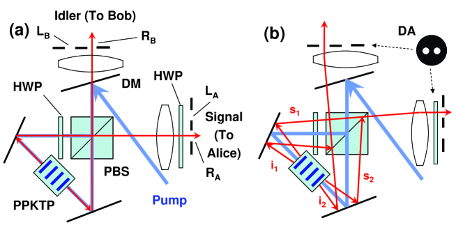
Figure 1: (Color online) Hyperentangled photon pair source in a PSI configuration, showing generation of polarization-entangled photon pairs in (a) collinear output modes along $R_{A}$ and $R_{B}$ and (b) non-collinear output modes along $L_{A}$ and $L_{B}$. The PSI consists of the crystal, two flat mirrors, a dual-wavelength half-wave plate (HWP), and a dual-wavelength polarizing beam splitter (PBS). The hyperentangled output state is a superposition of these two output modes each with a different probability amplitude. The two HWPs are used to rotate the polarizations by 90^∘. The subscripts 1 and 2 for the signal and idler outputs in (b) refer to the clockwise and counter-clockwise directions of the SPDC outputs, respectively. DM: dichroic mirror, DA: double aperture mask.

To generate the hyperentangled state that are entangled in both polarization and momentum degrees of freedom, we utilized a polarization-entangled photon pair source based on spontaneous parametric down-conversion (SPDC) in a type-II phase-matched periodically poled KTiOPO₄ (PPKTP) crystal in a bidirectionally pumped PSI configuration SagnacSource ; SagnacSource2 . The SPDC source was driven with $\sim$5 mW of a continuous-wave (cw) diode laser operating at a wavelength of 404.775 nm that was delivered to the PSI in a single-mode optical fiber. The 1-cm long PPKTP crystal was set at a temperature of $\sim$19 ^∘C for nearly frequency-degenerate operation. The signal and idler outputs at $809.55\pm 0.5$ nm were detected through 1-nm interference filters (IF) to restrict the SPDC output bandwidth. More details of the PSI source can be found in Ref. SagnacSource ; SagnacSource2 .

Normally the PSI entanglement source is operated in a collinearly propagating geometry for high collection efficiency of the polarization-entangled photons. However, it can also be operated in a slightly non-collinear configuration to exploit the momentum correlation of SPDC outputs. By collecting the non-collinear output modes from the PPKTP crystal the output photons are also momentum entangled MtmEntanglement ; PCNOT , as illustrated schematically in Fig. 1. After the PSI outputs are collimated the momentum of the output mode can be identified equivalently by its path location that is defined by the double-aperture (DA) mask. Unlike other hyperentanglement sources Hyperentangled1 ; Hyperentangled2 ; AVNExp2 , our experiment requires partial hyperentanglement with adjustable but equal amounts of entanglement in both polarization and momentum degrees of freedom, as indicated in Eq. (5). To control the degree of momentum entanglement ($\theta_{M}$), we aligned the DA mask at an asymmetric location with respect to the pump beam axis so that the right aperture ($R_{A}$ or $R_{B}$) coincided with the pump axis as shown in Fig. 1. The diameter of each aperture of the DA mask was 1 mm, and the distance between the centers of two apertures was 2 mm.

Consider the collinear $R_{A}$ and $R_{B}$ output modes of Fig. 1(a), which is the standard PSI configuration for generating polarization-entangled photons. We showed in previous PSI experiments SagnacSource ; SagnacSource2 that the output state is proportional to

$$|\psi\rangle_{R_{A}R_{B}}\equiv(\cos\theta_{P}\hat{a}_{H,R_{A}}^{\dagger}\hat{b}_{V,R_{B}}^{\dagger}+e^{i\phi}\sin\theta_{P}\hat{a}_{V,R_{A}}^{\dagger}\hat{b}_{H,R_{B}}^{\dagger})|0\rangle\,,$$ (7)

where $\hat{a}_{V,R_{A}}^{\dagger}(\hat{b}_{H,R_{B}}^{\dagger})$ is a $V$ ($H$) polarized photon creation operator for Alice’s $R_{A}$ (Bob’s $R_{B}$) path, and similarly for $\hat{a}_{V,R_{B}}^{\dagger}$ and $\hat{b}_{H,R_{A}}^{\dagger}$. The relative amplitude ($\theta_{P}$) and phase ($\phi$) of the output state are determined by the adjustable relative amplitude and phase between the $H$ and $V$ polarization components of the pump. Similarly, for the non-collinear $L_{A}$–$L_{B}$ output modes of Fig. 1(b), the output state is proportional to

$$|\psi\rangle_{L_{A}L_{B}}\equiv(\cos\theta_{P}\hat{a}_{H,L_{A}}^{\dagger}\hat{b}_{V,L_{B}}^{\dagger}+e^{i\phi}\sin\theta_{P}\hat{a}_{V,L_{A}}^{\dagger}\hat{b}_{H,L_{B}}^{\dagger})|0\rangle\,,$$ (8)

where $\theta_{P}$ and $\phi$ are the same as those in Eq. (7) because they are generated by the same pump laser.

For hyperentanglement, we consider the coherently driven outputs of all four paths and obtain a final state that is a superposition of the $|\psi\rangle_{R_{A}R_{B}}$ and $|\psi\rangle_{L_{A}L_{B}}$ outputs of Eq. (7) and Eq. (8), respectively. In general, the collinear output modes ($\hat{a}_{R_{A}}^{\dagger},\hat{b}_{R_{B}}^{\dagger}$) and the non-collinear output modes ($\hat{a}_{L_{A}}^{\dagger},\hat{b}_{L_{B}}^{\dagger}$) are excited with different probability amplitudes depending on the phase-matched emission angle ConeEntangle . Therefore, the four-path output is a partially hyperentangled state given by

$$\cos\theta_{M}|\psi\rangle_{L_{A}L_{B}}+\sin\theta_{M}|\psi\rangle_{R_{A}R_{B}}$$

$$= \cos\theta_{M}(\cos\theta_{P}|HL\rangle_{A}|VL\rangle_{B}+e^{i\phi}\sin\theta_{P}|VL\rangle_{A}|HL\rangle_{B})$$

$$+ \sin\theta_{M}(\cos\theta_{P}|HR\rangle_{A}|VR\rangle_{B}+e^{i\phi}\sin\theta_{P}|VR\rangle_{A}|HR\rangle_{B})$$

$$= (\cos\theta_{P}|H_{A}\rangle|V_{B}\rangle+e^{i\phi}\sin\theta_{P}|V_{A}\rangle|H_{B}\rangle)$$

$$\otimes(\cos\theta_{M}|L_{A}\rangle|L_{B}\rangle+\sin\theta_{M}|R_{A}\rangle|R_{B}\rangle)\,.$$

By varying the crystal phase-matching temperature to change the solid angle of the SPDC emission cone, one can adjust the flux ratio between the collinear output mode and the non-collinear output mode, thereby controlling $\theta_{M}$. We set the pump relative phase such that the output phase $\phi=0$, and the half-wave plate placed in Alice’s path in Fig. 1 was used to rotate Aice’s output polarization by 90^∘ to yield a partially hyperentangled output state given by Eq. (5). As an input state for Schmidt projection, we adjusted the pump relative amplitudes to set $\theta_{P}=\theta_{M}=\theta$.

III.2 Implementation of Schmidt projection

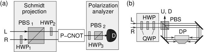
Figure 2: (Color online) Entanglement distillation scheme for hyperentangled photons. Alice and Bob have the same setup. (a) Schmidt projection transmits only the two relevant terms, $|VR\rangle$ and $|HL\rangle$, of the initial state given in Eq. (6). p-cnot gate combines two paths ($R$, $L$) into a common path for final state extraction and for polarization state analysis. (b) p-cnot gate with phase compensation. PBS: polarization beam splitter; HWP: half-wave plate; QWP: quarter-wave plate; DP: dove prism.

We applied single-qubit and two-qubit gates of single-photon two-qubit quantum logic to implement Schmidt projection on the partially hyperentangled state of Eq. (5), or its expanded form of Eq. (6). The SP procedure is to extract from the initial state the maximally entangled term $|\psi\rangle_{SP}=|VR\rangle_{A}|VR\rangle_{B}+|HL\rangle_{A}|HL\rangle_{B}$, which is orthogonal to the other two terms in Eq. (6). Therefore, $|\psi\rangle_{SP}$ can be simply isolated by using a polarization beam splitter to separate the polarizations and choosing the appropriate beam paths. However, the extracted state $|\psi\rangle_{SP}$ still contains four modes even though $V$ ($H$) is always associated with $R$ ($L$). It is more useful to convert the extracted state to a more familiar form such as the polarization triplet state

$$|\phi^{+}\rangle=|H_{A}H_{B}+V_{A}V_{B}\rangle/\sqrt{2}\,.$$ (9)

The transformation from $|\psi\rangle_{SP}$ to $|\phi^{+}\rangle$ can be accomplished with a polarization controlled not (p-cnot) gate PCNOT that converts $\psi\rangle_{SP}$ to $|\phi^{+}\rangle\otimes|L\rangle$, thus bringing the momentum qubit to a fixed value, which we can ignore in the final output state $|\phi^{+}\rangle$. The polarization-entangled triplet final state is much easier to analyze using polarization correlation measurements than dealing with a state containing both $L$ and $R$ paths.

Fig. 2(a) shows the apparatus for implementing the Schmidt projection method. The key step is to project the initial state given by Eq. (6) into a subspace composed of $|VR\rangle$ and $|HL\rangle$ for both Alice and Bob without destroying the qubits. In principle, this can be accomplished by using one PBS in the $L$ path to transmit the $H$-polarized photon in the $L$ path and another PBS in the $R$ path but is rotated by 90^∘ about the propagating axis to transmit the $V$-polarized photon in that path. The first two terms in Eq. (6) are then reflected. In the actual setup of Fig. 2 we modify this arrangement by using the HWP₁ to flip the polarization in the $R$ path before PBS₁ that transmits the desired subspace components in both paths. Instead of recovering the polarization state in the $R$ path after PBS₁, we flip the polarization state in the $L$ path with HWP₂, so that the output after Schmidt projection is $\cos\theta\sin\theta(|HR\rangle_{A}|HR\rangle_{B}+|VL\rangle_{A}|VL\rangle_{B})$. Note that HWP₁ and HWP₂ are essentially momentum-controlled not (m-cnot) gates described in Ref. SPTQSWAP . We should point out that the arrangement of having one HWP in each path eliminates the need for path-length compensation between the two paths that is necessary if only one m-cnot gate (i.e., a HWP) is used.

To eliminate the path dependence of the Schmidt-projected state $|HR\rangle_{A}|HR\rangle_{B}+|VL\rangle_{A}|VL\rangle_{B}$, we fold the $L$-path output and the $R$-path output onto a common path by use of a p-cnot gate, as indicated in Fig. 2(a). The final output state becomes $|\phi^{+}\rangle$ and we simplify the notation by removing the path designation. The implementation of this p-cnot gate is schematically shown in Fig. 2(b). The p-cnot gate consisted of a dove prism embedded in a polarization Sagnac interferometer that would rotate the incoming image ($L$ and $R$ beams) by $\pm 90^{\circ}$ depending on the beam polarization PCNOT . The p-cnot gate has the following mapping: $|HL\rangle\rightarrow|HU\rangle,|HR\rangle\rightarrow|HD\rangle,|VL\rangle\rightarrow|VD\rangle,|VR\rangle\rightarrow|VU\rangle$, where $U$ ($D$) refers to the upside (downside) path. For the purpose of relating to the usual $|0\rangle$ and $|1\rangle$ states, we identify $H$, $L$, and $U$ with $|0\rangle$, and $V$, $R$, and $D$ with $|1\rangle$. Our p-cnot implementation introduced a fixed amount of phase shifts depending on the input polarization SimAttackBB84 and they were compensated by adding a HWP sandwiched by two quarter-wave plates (QWPs) whose optic axes were tilted by 45^∘, as shown in Fig. 2(b). This phase compensator was also utilized to add the necessary $\pi/2$ phase shift in our quantum state tomography measurements in the next Section.

To verify that the final output is the maximally-entangled polarization triplet $|\phi^{+}\rangle$, we analyzed the polarization correlation between Alice’s and Bob’s coincidence counts. The polarization measurements were carried out with polarization analyzers each consisting of HWP₃, PBS₂, and a Si single-photon counter, as shown in Fig. 2(a). The measurement basis for the polarization analyzer was set by HWP₃.

IV EXPERIMENTAL RESULTS

Our implementation of the Schmidt projection protocol is best characterized by first demonstrating the required input hyperentangled state of Eq. (6) was generated and then measuring the degree of entanglement of the output state. Given a general hyperentangled state with arbitrary degrees of entanglement for the polarization and momentum qubit pairs of Eq. (5), $\theta_{P}=\theta_{M}=\theta$ is required for the input. In our verification of the input state, we characterized the partially hyperentangled state by comparing the different amounts of entanglement in the polarization and momentum modes at different $\theta=44^{\circ},41.9^{\circ},39.3^{\circ},35.9^{\circ}$. For each $\theta$ the SP protocol was carried out on the input state and we analyzed the extracted output state. In particular, we measured how close the extracted state was to the expected polarization triplet $|\phi^{+}\rangle$.

IV.1 Input state characterization

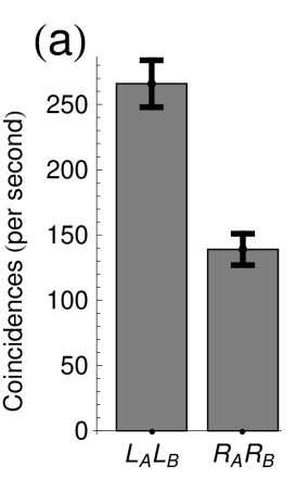
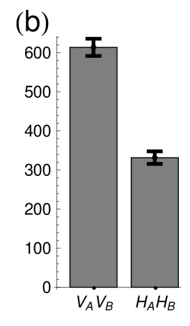
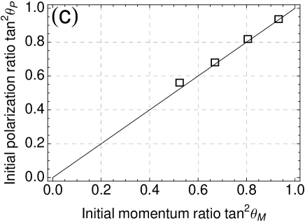
Figure 3: Characterization of initial hyperentangled state. Detected coincidences of (a) $|L\rangle_{A}|L\rangle_{B}$ and $|R\rangle_{A}|R\rangle_{B}$ terms for momentum input state $\theta_{M}=35.9^{\circ}$ ($\theta_{P}=45^{\circ}$), and (b) $|V\rangle_{A}|V\rangle_{B}$ and $|H\rangle_{A}|H\rangle_{B}$ terms for polarization input state $\theta_{P}=35.9^{\circ}$ ($\theta_{M}=45^{\circ}$). (c) Initial state of polarization qubits $\tan^{2}\theta_{P}$ as a function of initial state of momentum qubits $\tan^{2}\theta_{M}$. Open squares are the measurement results, and the straight line indicates the ideal case. Pump power was 5 mW, and detection bandwidth was 1 nm.

To characterize the input hyperentangled state of Eq. (5), we utilized the SP and p-cnot apparatus of Fig. 2(a) and our ability to control $\theta_{M}$ and $\theta_{P}$ independently, as described in Sect. III. The combination of the SP and p-cnot gate transforms the input state of Eq. (5) into

$$(\cos\theta_{P}\sin\theta_{M}|H\rangle_{A}|H\rangle_{B}+\sin\theta_{P}\cos\theta_{M}|V\rangle_{A}|V\rangle_{B})|D\rangle_{A}|D\rangle_{B}\,.$$ (10)

To evaluate the distribution of the momentum entanglement, we set $\theta_{P}=45^{\circ}$ in Eq. (10) so that $\cos\theta_{P}=\sin\theta_{P}=1/\sqrt{2}$. As discussed in Sect. III, we adjusted the relative $H$ and $V$ components of the pump to control $\theta_{P}$. We then obtained the ratio of $\sin^{2}\theta_{M}/\cos^{2}\theta_{M}$ by measuring the coincidence ratio of $C(H,H)$ and $C(V,V)$, where $C(X,Y)$ denotes the detected coincidence rate between $X$-qubit measurement by Alice and $Y$-qubit measurement by Bob. Any desired momentum entanglement distribution can be obtained by adjusting the SPDC crystal temperature while monitoring this coincidence ratio. Fig. 3(a) shows the measured distribution of the momentum qubits for $\theta_{M}=35.9^{\circ}$. For all the coincidence measurements in this work, each consisted of an average of 60 1-s measurements without background subtraction.

Similarly, to obtain the distribution of the polarization entanglement, we set $\theta_{M}=45^{\circ}$ by choosing an appropriate PPKTP temperature. After Schmidt projection and the p-cnot gate, we measured the polarization distribution by monitoring the coincidence ratio of $C(V,V)$ and $C(H,H)$ to yield $\tan^{2}\theta_{P}$. Fig. 3(b) shows the distribution of the polarization qubits for the case of $\theta_{P}=35.9^{\circ}$. Note that Fig. 3(a) and (b) have different scales because the two measurements were taken at two different temperatures that resulted in different output fluxes. More importantly is that Fig. 3(a) and (b) show that both ratios are nearly identical, as required by the Schmidt projection protocol.

The above measurements for determining the crystal temperature to obtain $\theta_{M}=35.9^{\circ}$ and the pump’s $H$–$V$ component ratio to set $\theta_{P}=35.9^{\circ}$ were repeated for other $\theta_{M}$ and $\theta_{P}$ values of $44^{\circ},41.9^{\circ}$, and $39.3^{\circ}$. Fig. 3(c) shows the measured polarization coincidence ratio $\tan^{2}\theta_{P}$ at various measured momentum coincidence ratio $\tan^{2}\theta_{M}$, showing clearly that the degree of partial entanglement in the polarization and momentum qubit pairs were well matched, $\theta_{M}\approx\theta_{P}$. The ideal distribution ratio is also shown in Fig. 3(c) as a straight line. To obtain the partially hyperentangled state required for the SP protocol (and for the measurements in Fig. 3(c)), we set $\theta_{M}=\theta_{P}=\theta$ in the following way. First, we set $\theta_{P}=45^{\circ}$ that could be confirmed by monitoring the coincidence ratio in the polarization qubits of the collinear $R$-path outputs. Then we adjusted the crystal temperature to the value that would yield the desired $\theta_{M}$, which we verified with the measurements presented in Fig. 3(a). Finally, we set $\theta_{P}$ to the same value as $\theta_{M}=\theta$ that we confirmed by again measuring the polarization coincidence ratio of the collinear $R$-path outputs.

IV.2 Characterization of Schmidt projected output state

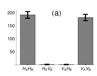
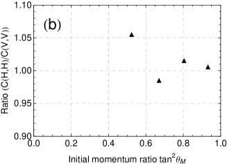
Figure 4: Coincidence measurements of output state in the $H$–$V$ basis. (a) Measured coincidence rate of the two parallel and two orthogonal polarization terms of the output state for input state with $\theta=35.9^{\circ}$. (b) Plot of $C(H,H)/C(V,V)$ of the output state as a function of initial momentum qubit ratio $\tan^{2}\theta_{M}$. Pump power was 5 mW, and detection optical bandwidth was 1 nm.

After the distillation procedure, we expect the final state to be a maximally polarization-entangled triplet state $|\phi^{+}\rangle$ of Eq. (9). We first analyzed the output state by measuring the coincidences between Alice and Bob in the $H$–$V$ basis, that for $|\phi^{+}\rangle$ should yield equal probability of detecting parallel polarizations but zero probability of detecting orthogonal polarizations. Fig. 4(a) shows the four measured coincidence rates $H_{A}H_{B}$, $H_{A}V_{B}$, $V_{A}H_{A}$, and $V_{A}V_{B}$ for an input state with $\theta\simeq 35.9^{\circ}$. The measurement results clearly show that the output state had nearly balanced $|H\rangle_{A}|H\rangle_{B}$ and $|V\rangle_{A}|V\rangle_{B}$ terms and negligible $|H\rangle_{A}|V\rangle_{B}$ and $|V\rangle_{A}|H\rangle_{B}$ components. We then made the same coincidence measurements for input states with different values of $\theta$. The coincidence rates for orthogonal polarizations $H_{A}V_{B}$ and $V_{A}H_{B}$ were negligible, as expected for $|\phi^{+}\rangle$. Fig. 4(b) plots the ratio of coincidence rates $C(H,H)/C(V,V)$ of the output state (solid triangles) as a function of the input state set by $\theta$. The measured coincidence ratios lie close to the expected value of unity for a maximally entangled output state with less than 5% error.

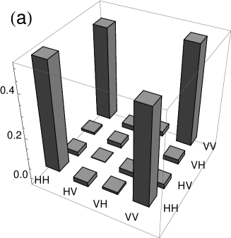
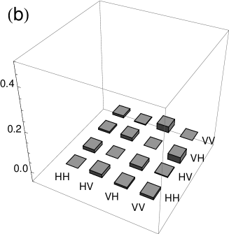
Figure 5: (a) Real part, and (b) imaginary part of measured density matrix of the Schmidt projected output state for initial state with $\theta=35.9^{\circ}$.

To show that the distilled output was indeed entangled as a coherent superposition, and not as a classical mixture, of $|H\rangle_{A}|H\rangle_{B}$ and $|V\rangle_{A}|V\rangle_{B}$, we made additional measurements for verification. We first performed quantum state tomography QTomography on the output state. We can reconstruct the density matrix of Alice’s and Bob’s polarization qubits by making coincidence measurements for the 16 combinations of their polarization analyzers set along $|H\rangle$, $|V\rangle$, $(|H\rangle+|V\rangle)/\sqrt{2}$, and $(|H\rangle-i|V\rangle)/\sqrt{2}$. The real and imaginary parts of the output density matrix $\rho$ for the case $\theta=35.9^{\circ}$ are displayed in Fig. 5(a) and (b), showing clearly that the state is $|\phi^{+}\rangle$ with a fidelity, $\langle\phi^{+}|\rho|\phi^{+}\rangle$, of 0.952.

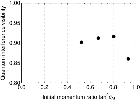
Figure 6: Measured quantum-interference visibilities in the $\pm 45^{\circ}$ diagonal basis $(|H\rangle\pm|V\rangle)$.

Another useful indicator of the output state coherence is two-photon quantum interference visibility measured in the $\pm 45^{\circ}$ diagonal basis $(|H\rangle\pm|V\rangle)$. Quantum interference visibility is defined as $(C_{max}-C_{min})/(C_{max}+C_{min})$, where $C_{max}$ is the maximum coincidence counts and $C_{min}$ is the minimum coincidence counts. Fig. 6 plots the measured visibilities for different input states, all showing $\sim$90% visibility except one lower-visibility point that was caused by a slight misalignment of the apparatus. The visibilities in Fig. 6 were primarily limited by the imperfect p-cnot gate that had a classical visibility of only $\sim$93% PCNOT . Another possible source of the visibility loss is the slight spectral mismatch of the output photons from the $L$ and $R$ output spatial modes. Even though the spectra of the output photons were mainly determined by the two interference filters, a slight mismatch in the filtered output spectra could happen because slightly different emission angles for the $L$ and $R$ paths (see Fig. 1) would yield slightly different spectral distribution.

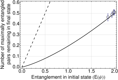
Figure 7: Measured efficiency of Schmidt projection implementation. Expected number of maximally entangled pairs after Schmidt projection is applied to a pair of hyperentangled state as a function of entanglement in the initial state ($E(\psi)$). Open circle is the measured number and the solid curve is the theoretical prediction when Schmidt projection is applied to a hyperentangled state. The dashed curve shows the maximum number of maximally entangle pairs obtainable by Schmidt projection when the input consists of an infinite number of pairs.

From the different state analysis measurement results shown in Fig. 4, 5, and 6, we conclude that our distillation outputs were in the $|\phi^{+}\rangle$ state independent of the input states with different $\theta$ values. One of the key advantages of the SP protocol is its high distillation efficiency, especially for a large number of initial pairs. We have measured the efficiency of our Schmidt projection implementation in terms of the expected number of maximally entangled pairs remaining in the final state as we varied the amount of initial entanglement $E(\psi)$ that we plot in Fig. 7 as open circles. We find that the measured efficiency is in good agreement with the theoretically calculated values (solid curve). For comparison, the dashed line in Fig. 7 shows the maximum number of maximally entangled pairs obtainable by the Schmidt projection protocol when it is applied to an infinite number of input pairs. In general, Schmidt projection shows a lower yield than Procrustean methods Concentration ; Procrustean when it is applied to less than 5 pairs, as in our case. However, even with a small number of initial pairs, Schmidt projection still has the practical advantage that it is not necessary to adjust the distillation setup as a function of the input states.

V DISCUSSION

In this work, we have experimentally demonstrated the Schmidt projection method that is considered one of the most powerful distillation protocols. We employed hyperentangled photons produced by spontaneous parametric down-conversion to generate pairs of partially-entangled states. We developed a technique to independently control the amount of entanglement in the polarization (by pump adjustments) and momentum (by crystal temperature) degrees of freedom of the hyperentangled photon pairs. This entanglement control capability was utilized to prepare the identical pairs of partially entangled qubits as the initial state for the SP protocol. Schmidt projection on the hyperentangled photon pairs was realized by a PBS and two m-cnot gates, and we used a p-cnot gate to convert the output into a polarization Bell state. Our experimental results show that Schmidt projection can distill a pair of maximally entangled qubits in the form of a polarization-entangled triplet and it is independent of the degree of entanglement in the initial state. Furthermore, the measured distillation efficiencies agree with the theoretical prediction. We note that Schmidt projection can be selectively applied to perform entanglement purification. If classical communication is used to compare the projection results, then certain types of mixed states can be purified, such as $\rho=\Sigma p|\psi\rangle\langle\psi|+(1-p)|01\rangle\langle 01|$, as well as a mixture of two identically decohered pairs Parity1 .

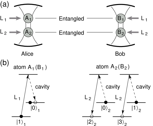
Figure 8: Schematic illustration of applying Schmidt projection to cQED. (a) Alice and Bob have two pairs of entangled atoms (A₁–B₁, A₂–B₂) trapped in an optical cavity. Pulses from two lasers, L₁ and L₂, are applied in a specific sequence to implement adiabatic transfer of the dark state cQED . (b) Proposed electronic-level structure for implementing the SP protocol. Atoms A₁ and A₂ are of the same kind (e.g., Rb BellMeasurement ), and different levels are used to encode the initial qubit state. After adiabatic passage, A₁ will be in the $|0\rangle_{1}$ state, and A₂ will be a superposition of all four states ($|0\rangle_{2}$–$|3\rangle_{2}$).

It is important to recognize that the key to our Schmidt projection implementation is that distinct tensor products of local qubits, $|0\rangle_{1}|0\rangle_{2}$, $|0\rangle_{1}|1\rangle_{2}$, $|1\rangle_{1}|0\rangle_{2}$, and $|1\rangle_{1}|1\rangle_{2}$, are encoded in physically distinguishable states, $|VL\rangle$, $|VR\rangle$, $|HL\rangle$, $|HR\rangle$. Therefore the same concept can be applied to other qubit systems such as cavity quantum electrodynamics (cQED) cQED ; BellMeasurement or trapped ion IonTrapCNOT systems, where multiple-qubit product states can be mapped into different internal states within the same atom. For example, in a cQED system illustrated in Fig. 8(a), Alice has two trapped atoms each of which is entangled with the corresponding trapped atom in Bob’s cavity, where the qubits are stored in the ground-state Zeeman levels. Consider the case in which the first qubit is stored in $|0\rangle_{1}$ and $|1\rangle_{1}$ of A₁ (B₁) and the second qubit is in $|0\rangle_{2}$ and $|1\rangle_{2}$ of A₂ (B₂) on Alice’s (Bob’s) side as shown in Fig. 8(a). One can coherently transfer the quantum states stored in Alice’s two atoms completely to A₂ while leaving A₁ in $|0\rangle_{1}$ by adiabatic passage via a dark state of the two-atom + cavity system cQED . That is, $|p\rangle_{1}|q\rangle_{2}\Rightarrow|0\rangle_{1}|p\,q\rangle_{2}$ when $p\,q$ is in a binary representation. By mapping all four possible quantum states into four internal states of A₂, the undesirable states such as $|0\rangle_{2}$ or $|3\rangle_{2}$ can be eliminated by driving the cycling transitions from the undesirable states to an auxiliary state (not shown in the level structure) BellMeasurement , and the process can be confirmed by the induced fluorescence. If no fluorescence is observed, we can conclude that Schmidt projection has successfully taken place.

In the trapped-ion case, one can use the quantized center-of-mass vibrational mode (‘bus mode’) in a similar way as in the cQED case. When there are two ions, the electronic state of the first ion can be transferred to the bus mode IonTrapCNOT with a red-sideband transition, and this bus mode can be transferred to the second ion while mapping four different two-qubit states to four distinct internal states of the second ion. The rest of the procedure is similar to the cQED case. We believe that further studies of Schmidt-projection implementations in atoms and ions and for mixed states should enhance our expanding collection of tools in quantum information science.

This work was partially supported by the Hewlett Packard-MIT Alliance.

References

- (1) C. H. Bennett, G. Brassard, C. Crépeau, R. Jozsa, A. Peres, and W. K. Wootters, Phys. Rev. Lett. 70, 1895 (1993).
- (2) E. Knill, R. Laflamme, and G. J. Milburn, Nature 409, 46 (2001).
- (3) D. Gottesman and I. L. Chuang, Nature 402, 390 (1999).
- (4) R. Raussendorf and H. J. Briegel, Phys. Rev. Lett. 86, 5188 (2001).
- (5) A. K. Ekert, Phys. Rev. Lett. 67, 661 (1991).
- (6) H. J. Briegel, W. Dür, J. I. Cirac, and P. Zoller, Phys. Rev. Lett. 81, 5932 (1998).
- (7) C. H. Bennett, H. J. Bernstein, S. Popescu, and B. Schumacher, Phys. Rev. A 53, 2046 (1996).
- (8) C. H. Bennett, G. Brassard, S. Popescu, B. Schumacher, J. A. Smolin, and W. K. Wootters, Phys. Rev. Lett. 76, 722 (1996); R. Reichle, D. Leibfried, E. Knill, J. Britton, R. B. Blakestad, J. D. Jost, C. Langer, R. Ozeri, S. Seidelin, D. J. Wineland, Nature 443, 838 (2006).
- (9) J. W. Pan, C. Simon, . Brukner, and A. Zeilinger, Nature 410, 1067 (2001).
- (10) R. T. Thew, and W. J. Munro, Phys. Rev. A 63, 030302(R) (2001).
- (11) W. Xiang-bin, and F. Heng, Phys. Rev. A 68, 060302(R) (2003); M. J. Hwang, and Y. H. Kim, Phys. Lett. A 369, 280 (2007).
- (12) P. G. Kwiat, S. Barraza-Lopez, A. Stefanov, and N. Gisin, Nature 409, 1014 (2001).
- (13) J. W. Pan, S. Gasparoni, R. Ursin, G. Weihs, and A. Zeilinger, Nature 423, 417 (2003).
- (14) T. Yamamoto, M. Koashi, and N. Imoto, Phys. Rev. A 64, 012304 (2001); T. Yamamoto, M. Koashi, S. Özdemir, and N. Imoto, Nature 421, 343 (2003).
- (15) Z. Zhao, J. W. Pan, and M. S. Zhan, Phys. Rev. A 64, 014301 (2001); Z. Zhao, T. Yang, Y. A. Chen, A. N. Zhang, and J. W. Pan, Phys. Rev. Lett. 90, 207901 (2003).
- (16) C. H. Bennett, D. P. DiVincenzo, J. A. Smolin, and W. K. Wootters, Phys. Rev. A 54, 3824 (1996).
- (17) W. K. Wootters, Phys. Rev. Lett. 80, 2245 (1998).
- (18) S. Hill and W. K. Wootters, Phys. Rev. Lett. 78, 5022 (1997).
- (19) S. P. Walborn, P. H. Souto Ribeiro, L. Davidovich, F. Mintert, and A. Buchleitner, Nature 440, 1022 (2006).
- (20) W. K. Wootters, Phil. Trans. R. Soc. Lond. A 356, 1717 (1998).
- (21) M. Fiorentino and F. N. C. Wong, Phys. Rev. Lett. 93, 070502 (2004).
- (22) M. Fiorentino, T. Kim, and F. N. C. Wong, Phys. Rev. A 72, 012318 (2005).
- (23) T. Kim, M. Fiorentino, and F. N. C. Wong, Phys. Rev. A 73, 012316 (2006).
- (24) F. N. C. Wong, J. H. Shapiro, and T. Kim, Laser Physics 16, 1517 (2006).
- (25) J. G. Rarity and P. R. Tapster, Phys. Rev. Lett. 64, 2495 (1990).
- (26) J. T. Barreiro, N. K. Langford, N. A. Peters, and P. G. Kwiat, Phys. Rev. Lett. 95, 260501 (2005).
- (27) M. Barbieri, C. Cinelli, P. Mataloni, and F. De Martini, Phys. Rev. A 72, 052110 (2005).
- (28) T. Yang, Q. Zhang, J. Zhang, J. Yin, Z. Zhao, M. Zukowski, Z. B. Chen, and J. W. Pan, Phys. Rev. Lett. 95, 240406 (2005).
- (29) M. Fiorentino, C. E. Kuklewicz, and F. N. C. Wong, Optics Express 13, 127 (2004).
- (30) T. Kim, I. Stork genannt Wersborg, F. N. C. Wong, and J. H. Shapiro, Phys. Rev. A 75, 042327 (2007).
- (31) J. B. Altepeter, D. F. V. James, and P. G. Kwiat, Lect. Notes Phys. 649, 113 (2004).
- (32) T. Pellizzari, S. A. Gardiner, J. I. Cirac, and P. Zoller, Phys. Rev. Lett. 75, 3788 (1995).
- (33) S. Lloyd, M. S. Shahriar, J. H. Shapiro, and P. R. Hemmer, Phys. Rev. Lett. 87, 167903 (2001).
- (34) J. I. Cirac and P. Zoller, Phys. Rev. Lett. 74, 4091 (1995).