Multifactor Analysis of Multiscaling in Volatility Return Intervals

Abstract

We study the volatility time series of 1137 most traded stocks in the US stock markets for the two-year period 2001-02 and analyze their return intervals $\tau$, which are time intervals between volatilities above a given threshold $q$. We explore the probability density function of $\tau$, $P_{q}(\tau)$, assuming a stretched exponential function, $P_{q}(\tau)\sim e^{-\tau^{\gamma}}$. We find that the exponent $\gamma$ depends on the threshold in the range between $q=1$ and $6$ standard deviations of the volatility. This finding supports the multiscaling nature of the return interval distribution. To better understand the multiscaling origin, we study how $\gamma$ depends on four essential factors, capitalization, risk, number of trades and return. We show that $\gamma$ depends on the capitalization, risk and return but almost does not depend on the number of trades. This suggests that $\gamma$ relates to the portfolio selection but not on the market activity. To further characterize the multiscaling of individual stocks, we fit the moments of $\tau$, $\mu_{m}\equiv\langle(\tau/\langle\tau\rangle)^{m}\rangle^{1/m}$, in the range of $10<\langle\tau\rangle\leq 100$ by a power-law, $\mu_{m}\sim\langle\tau\rangle^{\delta}$. The exponent $\delta$ is found also to depend on the capitalization, risk and return but not on the number of trades, and its tendency is opposite to that of $\gamma$. Moreover, we show that $\delta$ decreases with $\gamma$ approximately by a linear relation. The return intervals demonstrate the temporal structure of volatilities and our findings suggest that their multiscaling features may be helpful for portfolio optimization.

The study of volatility has long been one of the main topics of economics and econophysics research Mandelbrot63 ; Mantegna95 ; Kondor99 ; Mantegna00 ; Takayasu97 ; Bouchaud00 ; Johnson03 ; Liu99 ; Plerou01 . It is important for revealing the mechanism of price dynamics as well as for developing strategies of investment. For example, it helps the investor to estimate the risk and optimize the portfolio Bouchaud00 ; Johnson03 . As a stylized fact of econophysics, the volatility time series has long-term power-law correlations Liu99 ; Plerou01 ; Ding83 ; Wood85 ; Harris86 . The temporal structure in volatilities is complex and still regarded as an open problem. Return interval $\tau$, also called recurrence time or interspike interval, which is the time interval between two consecutive volatilities above a certain threshold $q$, provides a new approach to analyze long-term correlated time series Altmann05 ; Yamasaki05 ; Wang06 ; Weber07 ; Vodenska08 ; Jung08 ; Bunde04 ; Livina05 ; Lennartz08 ; Eichner07 ; Bogachev07 ; Wang08 . Recent studies on financial markets Yamasaki05 ; Wang06 ; Weber07 ; Vodenska08 ; Jung08 show that, for both daily and intraday data, i) the distribution of scaled interval $\tau/\langle\tau\rangle$ can be approximated by a single scaling function, where $\langle\tau\rangle$ is the average of $\tau$. The scaling function can also be approximated by a stretched exponential (SE) function. ii) The sequences of the return intervals have long-term memory which is related to the long-term correlations in the original volatility sequences. Similar findings are observed for other long-term correlated time series, such as climate and earthquake Bunde04 ; Livina05 ; Lennartz08 . Also there are some related studies on financial markets, such as first passage time Masoliver05 and level crossing Jafari06 .

As a typical complex system, financial market is composed of many interconnected participants and its time series is usually not of uniscaling nature Matteo07 . Market activity such as the intertrade time shows multiscaling in its distribution Ivanov04 ; Eisler06 . Recently we suggested that the return intervals distribution has multiscaling characteristics based on cumulative distributions and moments of scaled intervals for 500 constituents of the Standard & Poor’s 500 index Wang08 . The following questions are, can we detect multiscaling for a broader market? More important, what is the reason for multiscaling in the return intervals? Is it related to the market activity? Or is it connected to the portfolio selection criteria such as company size, stock risk or return? The study of those possible relations may shed light on the underlined mechanism of the volatility and may help investors to optimize their portfolio.

In this paper we analyze the volatility return intervals of the entire US stock markets. The database analyzed is the Trades And Quotes (TAQ) from New York Stock Exchange (NYSE). The period studied is from Jan 1, 2001 to Dec 31, 2002, totally 500 trading days. TAQ records every trade (“tick”) for all securities in the US stock markets. The stock activity varies in a wide range, between $5$ and $65,000$ trades per day. For constructing a minute resolution data, one need enough records in every day and thus we choose only stocks that have at least 500 daily trades. With this criterion, we obtain 1137 stocks which are the most traded in the market. From tick prices we set the closest one to a minute mark as the price at that minute. The volatility is defined the same as in Ref Wang06 . First, we compute the absolute value of the logarithmic change of the minute price, then remove the intraday U-shape pattern, and finally normalize the series with its standard deviation. Therefore the volatility is in units of standard deviations. Since the sampling time is 1 minute, a trading day has 390 points (after removing the market closing hours), and each stock has about 195,000 records.

The analysis with respect to several essential factors is widely used in economics studies. For instance, company size, market return and book-to-market value are used to model asset pricing Fama96 . Volatilities and therefore return intervals may be affected by many factors. Here we study how the return intervals distribution depends on a few essential measures which characterize different features of the stocks. The first one is the size of company, which is a popular criterion for portfolio selection. Stocks of different scales are preferred by investors of different types. The size also limits the group of investors and market depth for a stock. On the other hand, the internal organization of a company might dramatically varies with its size. Thus, the volatility and its return interval may be strongly influenced by this factor. The size is usually characterized by the market capitalization, product of the stock price and outstanding shares. Without loss of generality, we choose the price and outstanding shares on Dec 31, 2002 to calculate the capitalization. For the 1137 stocks, the range of capitalization is between $2\times 10^{7}$ and $2\times 10^{11}$ dollars.

The reward and risk are basic concerns for any investment and we therefore choose them as the next two factors. The reward is usually measured as the average return of price while risk is measured as the standard deviation of the return Markowitz52 . This traditional definition of the risk is based on the Gaussian distribution of the time series, which is not always adapted to the financial data Bouchaud00 . Nevertheless, it characterizes the magnitude of fluctuations and therefore the risk. To avoid the intraday pattern Liu99 ; Wang06 , we calculate the return on a daily basis. The return is the logarithmic daily price change averaged over the two-year period (2001-2002), which varies from $-0.008$ to $0.004$ for the 1137 stocks. The risk, standard deviation of daily returns in the two years, ranges from $0.012$ to $0.12$. The fourth factor we study is an activity measure, the number of trades per day. Note that the four factors reflect different aspects of a stock. The size is for the scale of company. The return and risk are historical price movement tendency and variation, which are helpful for the prediction of future price change. While the number of trades shows the activity, i.e., how frequent a stock is traded.

For a volatility time series, we choose a positive value as the threshold $q$ and find those volatilities above $q$, which are called “events”. Note that $q$ is in units of standard deviations. Then we calculate the time intervals $\tau$ between two consecutive events and compose a new time series. For each threshold $q$ we have a corresponding time series of return intervals. For financial markets, the PDF of $\tau$, $P_{q}(\tau)$, is well-approximated by the scaling function Yamasaki05 ; Wang06 ,

$$P_{q}(\tau)=\frac{1}{\langle\tau\rangle}f(\tau/\langle\tau\rangle),$$ (1)

where $\langle\cdot\rangle$ stands for the average over the data set. The scaling function $f(x)$, where $x$ corresponds to the scaled interval $\tau/\langle\tau\rangle$, can be approximated by a SE function,

$$f(x)=ce^{-(ax)^{\gamma}},$$ (2)

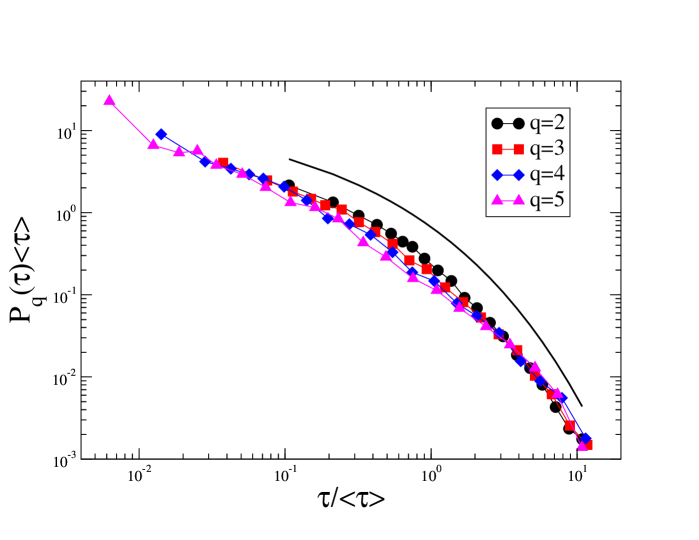
Figure 1: (Color online) Return interval PDFs of four thresholds, $q=2$, $3$, $4$ and $5$ for the GE stock. These four curves approximately collapse onto a single one, and the scaling function is approximate stretched exponential, as guided by the black curve which is the SE fitting to the data for $q=2$ (shifted vertically for better visibility).

in consistent with other long-term correlated records Bunde04 ; Altmann05 . The normalization constant $c$ and the scaled parameter $a$ depend on the exponent $\gamma$, and thus $f(x)$ has only one free parameter Altmann05 ; Wang08 . When the record has no long-term correlations, the return intervals follow as expected an exponential distribution, i.e. $\gamma=1$. As an example, we plot in Fig. 1 the PDFs of return intervals for a typical stock, General Electric (GE). The PDFs for four values of $q$ ($q=2$ to $5$) almost collapse onto a single curve. We also plot a SE (Eq. (2) fitting of the curve for $q=2$. For small values of $\tau$, there are some deviations from the SE function. Eichner et al. suggested that the scaling function is characterized by a power-law function for short time scales and a SE function for long time scales Eichner07 . To avoid these deviations, we analyze the scaling function only for large scales ($\tau/\langle\tau\rangle\geq 0.1$).

In a recent paper Wang08 , indications of deviations from the scaling function Eq. (2) were observed for the return intervals. The cumulative distributions for different thresholds $q$ were found to systematically deviate from a single scaling function Wang08 . This indicates that the exponent $\gamma$ may change with the threshold $q$. To test this assumption quantitatively and over the entire market, we compute $\gamma$ for all 1137 stocks and plot in Fig 2 their averages and standard deviations (as error bars) as a function of $q$. The values of $\gamma$ are obtained from the least-squares fit of the scaling function, Eq. (2), to the data for the range $\tau/\langle\tau\rangle\geq 0.1$ (see Fig. 1). The range of $q$ studied is from $1$ to $6$ with steps of $0.25$. We consider a point as on outlier if its RMS error is larger than $10\%$. Totally $730$ out of $22740$ points or $3.8\%$ of all points are removed. Fig. 2 shows that the mean $\gamma$ decreases with $q$, from $0.49$ for $q=1$ to $0.28$ for $q=3$. For large thresholds (between $q=3$ and $6$) $\gamma$ tends to be constant (around $0.26$), where the distribution can be regarded as close to be of uniscaling nature. The difference in $\gamma$ between small and large thresholds suggests multiscaling in the distribution for the whole range. The volatility time series has long-term correlations, which can be characterized by the exponent $\alpha$ obtained from Detrended Fluctuation Analysis (DFA) method Peng94 ; Liu99 ; Yamasaki05 ; Wang06 . Assuming the validity of the relation between $\gamma$ in Eq. (2) and the long-term correlations in the volatilities Eichner07 , $\alpha=1-\gamma/2$, it follows that small volatilities have large $\gamma$ and weak correlations, while large volatilities have small $\gamma$ and strong correlations. Large volatilities correspond to long time scales and small volatilities correspond to short time scales. The changes in the value of $\gamma$ seen in Fig. 2 might be due to the changes in the $\alpha$ found between short and long time scales in the volatility records Liu99 ; Wang06 . The error bars shown in Fig. 2 are limited for all thresholds, which indicates the tendency is consistent for the entire market. Note that error bars for several largest thresholds such as $q=6$ and $5.75$ are slightly larger, probably due to the bad statistics of fewer events.

Next we study the relations between $\gamma$ and the four essential factors, market capitalization, risk, number of trades and return. This tests the universality of $\gamma$ over the entire market. If $\gamma$ is sensitive to some factors, the market as one system is not of uniscaling. Furthermore, the dependence (if exist) may indicate some origins for the multiscaling found in return interval distributions. In Fig. 3, we plot $\gamma$ against the four factors for four thresholds, $q=2$, $3$, $4$ and $5$. In each panel, curves have similar tendency and the value of $\gamma$ decreases with $q$. Note that the curves are closer to each other for large thresholds. This finding is consistent with Fig. 2, which shows that the mean $\gamma$ decreases with $q$ and reaches almost a constant value for large $q$. More important, Fig. 3 exhibits that $\gamma$ for a given threshold is not uniformly distributed with the factor values and thus the market is of multiscaling nature.

For the company size (Fig. 3(a)), $\gamma$ increases for sizes between $5\times 10^{7}$ to $2\times 10^{10}$ dollars and then shows a slight decrease. The market depth for small companies limits the size of investors and those companies usually attract some specific types of investors. Therefore corresponding strategies may be relatively similar and the volatility series tends to be strongly correlated having a small $\gamma$ Bunde04 . With increasing size, more investors are involved, which may “randomize” the long-term correlations in volatilities. When the company size reaches a certain limit, the constitution of investor types may be relatively stable, some common modes might dominate volatilities and therefore the correlations become stronger and $\gamma$ decreases with the size.

Fig. 3(b) shows that $\gamma$ decreases with the risk except for very low risks. Fig. 2 shows that larger volatilities tend to have smaller $\gamma$. Larger risk means that the probability of larger volatilities is higher. Therefore, Fig. 3(b) is consistent with Fig. 2. Price movement is realized by trades and the temporal structure of the volatility probably relates to the size of trades. Counterintuitively, $\gamma$ is almost not sensitive to the market activity. Fig. 3(c) suggests no apparent dependence between $\gamma$ and the number of trades Note1 , see also Ivanov04 . A possibly reason is that many investors do not change their strategies only because of the dramatic change of trading frequency. Next we show in Fig. 3(d) the relation between $\gamma$ and the return. For negative returns $\gamma$ increases and decreases for positive returns. It has a maximum when the return is $0$. This behavior suggests that the return is related to the size of risk. For returns with large magnitude representing high volatilities, the corresponding risk is relatively high and therefore $\gamma$ is small (see Fig. 3(b)).

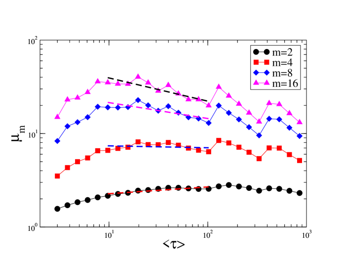
Figure 4: (Color online) Typcial moments $\mu_{m}$ of the GE stock. Four orders, $m=2$, $4$, $8$ and $16$ are shown. Dashed lines are power-law fittings in the range of $10<\langle\tau\rangle\leq 100$ for determining the multiscaling exponent $\delta$.

Next we study the multiscaling behavior of individual stocks. The moments of scaled interval, $\tau/\langle\tau\rangle$, can quantify the deviations from a single scaling function and therefore provide a good measure to test the multiscaling in individual stocks. In Fig. 4, we plot $\mu_{m}$ for GE as an example. The moment and the corresponding exponent $\delta$ for the multiscaling are defined as

$$\mu_{m}\equiv\langle(\tau/\langle\tau\rangle)^{m}\rangle^{1/m}\sim\langle\tau\rangle^{\delta}.$$ (3)

If the distribution of the return intervals follows a unique scaling law as Eq. (1), the different moments should be independent on $\langle\tau\rangle$ and therefore the exponent $\delta$ should be $0$. A significant $\delta$ suggests multiscaling, and the value of $\delta$ characterizes the strength of the multiscaling Wang08 , thus we call $\delta$ multiscaling exponent Note2 . We find that $\mu_{m}$ changes systematically with $\langle\tau\rangle$. For $m\geq 2$, moments first increase with $\langle\tau\rangle$ and then decrease Wang08 (for a typical example, see Fig. 4). Since a value of $\langle\tau\rangle$ corresponds to a threshold value $q$, the moments have the same trend with $q$. Here we choose four typical orders for moments, $m=2$, $4$, $8$ and $16$. For other positive orders, we find similar behaviors. For these four orders, all 1137 stocks totally have 215 out of 4548 cases ($4.7\%$) where the RMS error of fitting are over $22\%$, and are not included in the analysis.

Now we focus on the relation between the multiscaling exponent $\delta$ and the four factors. We plot in Fig. 5 the curves for four orders, $m=2$, $4$, $8$ and $16$. These curves have the similar tendency in each panel. The value of $\delta$ increases a little from $m=2$ to $4$, then decreases, which is consistent with the result in Ref Wang08 . As shown in Fig. 5(a), $\delta$ decreases with the capitalization until about $2\times 10^{10}$ dollars and then the curves increase. This suggests that $\delta$ also relates to the constitution of investors. A small company has few investors which have some specific strategies. However, if the company is very large, some types of investors finally dominate the price movement. In Fig. 5(b), $\delta$ increases almost monotonically with the risk, indicating that if a stock has larger volatility values, its return interval distribution has stronger multiscaling effect. Similar to $\gamma$, $\delta$ is almost independent on the number of trades as shown in Fig. 5(c). In Fig. 5(d), $\delta$ has a minimum at zero returns, which also agrees with the relation between $\delta$ and risk.

There are clear connections between Fig. 3 and Fig 5, which indicate that $\gamma$ and $\delta$ are strongly related. From Fig. 2, $\gamma$ decreases with $q$, a $q$ value corresponds to a $\langle\tau\rangle$ value, and $\delta$ is the power-law fitting exponent for the moment vs. $\langle\tau\rangle$. To examine the relation between the two exponents we plot $\delta$ against $\gamma$ in Fig. 6. Our results suggest that $\delta$ decreases with $\gamma$ for all four thresholds $q=2$, $3$, $4$ and $5$ when $m=2$. These curves approximately follow a linear function as guided by the dashed lines with the slope $-0.63$, $-0.75$, $-0.74$ and $-0.62$ respectively. Other thresholds $q$ and orders $m$ show similar results. The smaller is the value of $\gamma$, the larger deviation from a single scaling function for the return interval distribution is observed.

The SE exponent $\gamma$ characterizes the return intervals, which depend on the temporal structure of volatility time series. In other words, $\gamma$ characterizes the dynamic property of volatility. Capitalization, risk and return are fund mental measures of a company while number of trades is for the market activity, which is due to the market participants and not influenced by the company managers. We show that $\gamma$ relates to these fundamental measures but not to the activity. We also test the relation between $\gamma$ and share volume, and find no clear dependence, similar to that for number of trades. Although there is a certain relation between those measures, for instance, the number of trades depends on the capitalization Eisler06 , it does not guarantee that $\gamma$ depend on the number of trades. For a company of a given number of trades, its capitalization has a range of values, and for a company of a given capitalization, its $\gamma$ also distributes in a certain interval. Since there is a crossover in the curve of $\gamma$ and capitalization, it is possible that $\gamma$ is not sensitive to the number of trades. Capitalization, risk and return are widely used for building portfolio. Therefore, $\gamma$ connects the dynamic structure of the price movement with fundamental measures, which may provides an helpful indicator for portfolio selection. Similarly, the multiscaling exponent $\delta$ also could be used to optimize the portfolio. Recently Bogachev et al. studied return intervals in multifractal data sets and suggested that the return interval follows a power-law distribution Bogachev07 . Meanwhile, Livina et al. suggested a Gamma distribution for earthquake time series which also has long-term correlationsLivina05 . Therefore a detailed analysis on the distribution function is needed.

In summary, we analyzed the volatility return interval for 1137 most traded stocks in the United States markets. We have shown that the SE exponent $\gamma$ depends on the threshold $q$, which supports multiscaling nature in the return interval distribution. We also studied the relation between $\gamma$ and four essential factors of stock, capitalization, risk, number of trades and return. We found that $\gamma$ depends on the capitalization, risk and return but not on the number of trades, which suggests the multiscaling in the entire market. We further analyzed the multiscaling exponent $\delta$, which characterizes the multiscaling of individual stocks. We found that it again depends on the capitalization, risk and return but not on the number of trades. Our results suggest that $\delta$ and $\gamma$ may be useful for portfolio optimization.

We thank S.-J. Shieh, R. Mantegna, J. Kertész and Z. Eisler for helpful discussions, and the NSF and Merck Foundation for financial support.

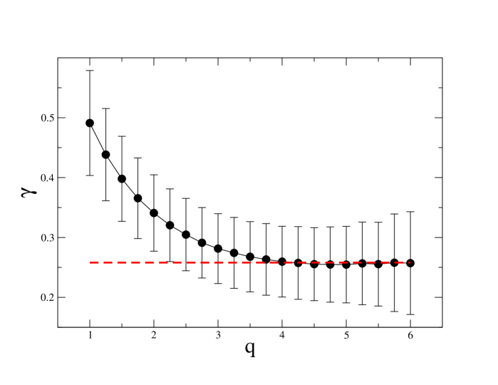
Figure 2: (Color online) SE exponent $\gamma$ vs. threshold $q$. The filled circles are the values of $\gamma$ averaged over 1137 most traded stocks and the error bars are the corresponding standard deviations. The dashed line is a guide line of $\gamma=0.26$.

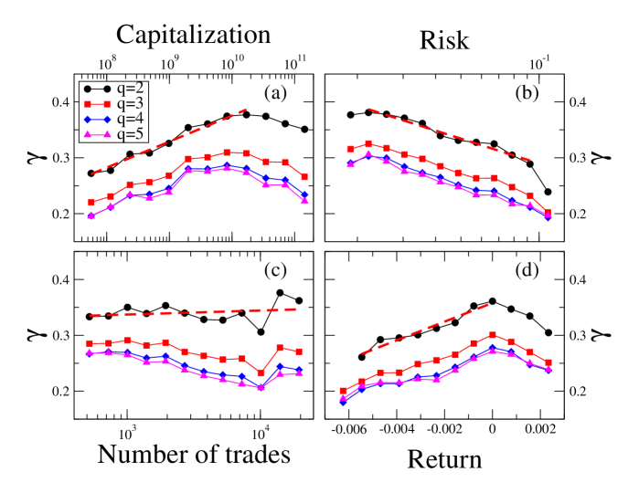
Figure 3: (Color online) Relation between SE exponent $\gamma$ and four factors: (a) market capitalization, (b) risk, the standard deviation of daily return, (c) average daily number of trades and (d) average daily return. Curves of four thresholds $q=2$, $3$, $4$ and $5$ are demonstrated. Dashed lines are logarithmic fittings (except for (d) where the fitting is linear) on the curve of $q=2$.

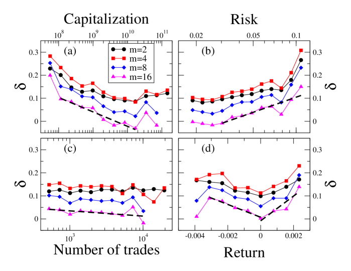
Figure 5: (Color online) Relation between multiscaling exponent $\delta$ and four factors: (a) market capitalization, (b) risk, the standard deviation of daily return, (c) average daily number of trades and (d) average daily return. Curves of four moments, $m=2$, $4$, $8$ and $16$ are shown. Dashed lines are fittings on the curve of $m=16$ which demonstrate the tendency.

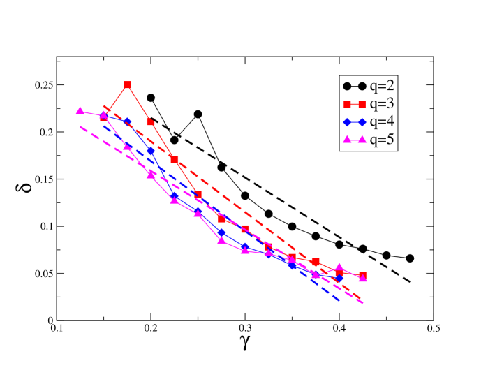
Figure 6: (Color online) Multiscaling exponent $\delta$ vs. SE exponent $\gamma$. The values of $\delta$ are for order $m=2$ and $\gamma$ are for thresholds $q=2$, $3$, $4$ and $5$. Linear fittings are shown by dashed lines.

References

- (1) B. B. Mandelbrot, J. Business 36, 394 (1963).
- (2) R. N. Mantegna and H. E. Stanley, Nature (London) 376, 46 (1995).
- (3) Econophysics: An Emerging Science, edited by I. Kondor and J. Kertész (Kluwer, Dordrecht, 1999).
- (4) R. Mantegna and H. E. Stanley, Introduction to Econophysics: Correlations and Complexity in Finance (Cambridge Univ. Press, Cambridge, England, 2000).
- (5) H. Takayasu et al., Physica A 184, 127 (1992); H. Takayasu et al., Phys. Rev. Lett. 79, 966 (1997); H. Takayasu et al., Fractals 6, 67 (1998).
- (6) J.-P Bouchaud and M. Potters, Theory of Financial Risk: From Statistical Physics to Risk Management (Cambridge Univ. Press, Cambridge, 2000).
- (7) N. F. Johnson, P. Jefferies, and P. M. Hui, Financial Market Complexity (Oxford Univ. Press, New York, 2003).
- (8) Y. Liu, P. Gopikrishnan, P. Cizeau, M. Meyer, C.-K. Peng, and H. E. Stanley, Phys. Rev. E 60, 1390 (1999).
- (9) V. Plerou et al., Quant. Finance 1, 262 (2001); V. Plerou et al., Phys. Rev. E 71 , 046131 (2005).
- (10) Z. Ding, C. W. J. Granger and R. F. Engle, J. Empirical Finance 1, 83 (1983).
- (11) R. A. Wood, T. H. McInish, and J. K. Ord, J. Finance 40, 723 (1985).
- (12) L. Harris, J. Financ. Econ. 16, 99 (1986).
- (13) A. Bunde et al., Physica A 342, 308 (2004); A. Bunde et al., Phys. Rev. Lett. 94, 048701 (2005).
- (14) V. N. Livina, S. Havlin, and A. Bunde, Phys. Rev. Lett. 95, 208501 (2005).
- (15) S. Lennartz, V. N. Livina, A. Bunde and S. Havlin, Europhys. Lett. 81, 69001 (2008).
- (16) E. G. Altmann and H. Kantz, Phys. Rev. E 71, 056106 (2005).
- (17) K. Yamasaki, L. Muchnik, S. Havlin, A. Bunde, and H. E. Stanley, Proc. Natl. Acad. Sci. U.S.A. 102, 9424 (2005).
- (18) F. Wang et al., Phys. Rev. E 73, 026117 (2006); F. Wang et al., Eur. Phys. J. B 55, 123 (2007).
- (19) P. Weber, F. Wang, I. Vodenska-Chitkushev, S. Havlin and H. E. Stanley, Phys. Rev. E 76, 016109 (2007).
- (20) I. Vodenska-Chitkushev, F. Wang, P. Weber, K. Yamasaki, S. Havlin, and H. E. Stanley, Eur. Phys. J. B 61, 217 (2008).
- (21) W.-S. Jung, F. Wang, S. Havlin, T. Kaizoji, H.-T. Moon and H. E. Stanley, Eur. Phys. J. B 62, 113 (2008).
- (22) J. F. Eichner, J. W. Kantelhardt, A. Bunde, and S. Havlin, Phys. Rev. E 75, 011128 (2007).
- (23) M. I. Bogachev, J. F. Eichner, and A. Bunde, Phys. Rev. Lett. 99, 240601 (2007).
- (24) F. Wang, K. Yamasaki, S. Havlin and H. E. Stanley, Phys. Rev. E 77, 016109 (2008).
- (25) J. Masoliver, M. Montero, and J. Perelló, Phys. Rev. E 71, 056130 (2005).
- (26) G. R. Jafari, M. S. Movahed, S. M. Fazeli, M. Reza Rahimi Tabar, and S. F. Masoudi, J. Stat. Mech.: Theory Exp. (2006), P06008.
- (27) T. Di Matteo, Quant. Finance 7, 21 (2007).
- (28) P. Ch. Ivanov, A. Yuen, B. Podobnik, and Y. Lee, Phys. Rev. E 69, 056107 (2004).
- (29) Z. Eisler et al., Phys. Rev. E 73, 046109 (2006); Z. Eisler et al., Eur. Phys. J. B 51, 145 (2006).
- (30) E. F. Fama and K. R. French, J. Finance 51, 55 (1996).
- (31) H. Markowitz, J. Finance 7, 77 (1952).
- (32) C.-K. Peng et al., Phys. Rev. E 49, 1685 (1994); C.-K. Peng et al., Chaos 5, 82 (1995).
- (33) Note that there is a slight tendency in Fig. 3(c), which is negligible if we compare it with the trends in other panels. As an example, the logarithmic fitting on the curve for (shown by dash lines in Fig. 3) has a slope of for the capitalization, for the risk, but only for the number of trades. Similar results are shown in Fig. 5.
- (34) To avoid the discreteness for small and finite size effects for large Wang08 , we choose the range of , for which a least-squares fit of a power-law function is performed. For the 1137 stocks studied, corresponds to threshold and corresponds to .