Oblique Ion Two-Stream Instability in the Foot Region of a Collisionless Shock

Abstract

Electrostatic behavior of a collisionless plasma in the foot region of high Mach number perpendicular shocks is investigated through the two-dimensional linear analysis and electrostatic particle-in-cell (PIC) simulation. The simulations are double periodic and taken as a proxy for the situation in the foot. The linear analysis for relatively cold unmagnetized plasmas with a reflected proton beam shows that obliquely propagating Buneman instability is strongly excited. We also found that when the electron temperature is much higher than the proton temperature, the most unstable mode is the highly obliquely propagating ion two-stream instability excited through the resonance between ion plasma oscillations of the background protons and of the beam protons, rather than the ion acoustic instability that is dominant for parallel propagation.

To investigate nonlinear behavior of the ion two-stream instability, we have made PIC simulations for the shock foot region in which the initial state satisfies the Buneman instability condition. In the first phase, electrostatic waves grow two-dimensionally by the Buneman instability to heat electrons. In the second phase, highly oblique ion two-stream instability grows to heat mainly ions. This result is in contrast to previous studies based on one-dimensional simulations, for which ion acoustic instability further heats electrons.

The present result implies that overheating problem of electrons for shocks in supernova remnants is resolved by considering ion two-stream instability propagating highly obliquely to the shock normal and that multi-dimensional analysis is crucial to understand the particle heating and acceleration processes in shocks.

1 Introduction

The discovery of thermal and synchrotron X-rays from young supernova remnants (SNRs) provides the evidence that electrons are heated up to a few keV and that a portion of them are accelerated to highly relativistic energy in SNR shocks (Koyama et al., 1995). Because SNR shocks are collisionless, not only particle acceleration mechanisms but also electron heating mechanisms in SNR shocks are not so simple. Previous studies have given an important key to the formation mechanism of perpendicular collisionless shocks. When the Alfv${\rm\acute{e}}$n Mach number $M_{\rm A}$ is larger than the critical Mach number, about 3, a perpendicular shock reflects some of the incident ions to the upstream, where a foot region forms on a spatial scale of the ion gyroradius (Leroy, 1983). The plasma in the foot region consists of incident ions and electrons and reflected ions and returning ions which are made from reflected ions and move to the shock after a gyration. As for the electron heating machanism, Papadopoulos (1988) proposed that when the Mach number is larger than $0.5(m_{\rm p}/m_{\rm e})^{1/2}\sim 20$, incident electrons and reflected ions excite electrostatic waves by the Buneman instability (Buneman, 1958) because the relative velocity between them is large compared with the electron thermal velocity. They also suggest that after electrons are heated by electrostatic waves induced by the Buneman instability, ion acoustic instability is triggered because the electron temperature becomes much higher than the proton temperature. As a result, electrons are strongly heated by the Buneman instability and the ion acoustic instability. Cargill & Papadopoulos (1988) performed a one-dimensional hybrid simulation and demonstrated that strong electron heating actually occurs. They concluded that an $M_{\rm A}=500$ shock heats electrons by a factor of $10^{5}$ across the shock. This means that if the upstream electron temperature is 1 eV, the downstream electron temperature becomes 100 keV. This value of the downstream temperature is much larger than the recent observational one for SNRs, a few keV (Stage et al., 2006). This discrepancy has been an open issue to be resolved for a long time.

On the other hand, Shimada & Hoshino (2000) and Hoshino & Shimada (2002) performed one-dimensional full particle-in-cell (PIC) simulations to investigate the electron acceleration at perpendicular shocks. Their simulation solves a whole region of a collisionless perpendicular shock and makes reflected ions self-consistently by employing a small proton to electron mass ratio. Their results showed that electrons are not only heated at the foot region but also significantly accelerated by surfing acceleration mechanism. However, this acceleration is valid only for the one-dimensional case because the surfing acceleration strongly depends on the structure of the electrostatic potential. In our first paper (Ohira & Takahara, 2007), we performed two-dimensional electrostatic PIC simulations to solve for the two-dimensinal structure of the electrostatic potential excited by the Buneman instability. We employed the real mass ratio but the simulation region is limited to the foot region. Our results showed that oblique modes grow as strongly as the modes parallel to the beam direction, that the potential structure becomes two-dimensional and that no efficient surfing acceleration occurs, while electron heating occurs. Thus, the problem of electron acceleration has been back to the start again. In that paper, we concentrated on the stage of the Buneman instability and did not follow the long time scale evolution after the Buneman nstability has saturated.

In this paper, we study the time evolution of electrostatic collisionless plasma instabilities in the foot region by making linear analysis and by performing two-dimensional electrostatic PIC simulation. We perform simulations with a higher resolution, a larger simulation box and a longer simulation time than in Ohira & Takahara (2007). Especially, we focus on the evolution after electrostatic waves excited by the Buneman instability have decayed. Our simulation substantially improves most previous works that are one-dimensional, employ an artifically small proton electron mass ratio or impose rather strong magnetic field. It is obvious that a multi-dimensional analysis is necessary as discussed above (Bludman et al, 1960; Lampe et al., 1974; Ohira & Takahara, 2007). Our motivation for employing the real mass ratio is as follows. For a small mass ratio, the foot region in the simulation is shorter than the realistic one and the time scale on which electrons stay in the foot region in the simulation is also shorter than the realistic one because the size of the foot region is about the ion gyroradius $m_{\rm p}v_{\rm d}c/eB$, where $v_{\rm d}$ and $B$ are the drift velocity of reflected protons and the magnetic field, respectively. Because reflected ions have a large free energy, we expect that more energy is transported to electrons through collective instabilities with the realistic mass ratio in the foot region. The drift velocity is not large enough to excite electromagnetic waves, so that electrostatic waves are more important.

In §2 we perform linear analysis for two-dimensional electrostatic modes. In §3 we describe the initial setting of the PIC simulations and numerical results, followed by a discussion in §4.

2 Linear analysis

In this section, we perform linear analysis for two-dimensional electrostatic modes in unmagnetized plasmas with beams. In the foot region of perpendicular shocks of SNRs, we regard that there are several beams with a finite temperature and that their relative velocities are much smaller than the light speed. Therefore, the fastest growing modes are electrostatic modes. Then, we here concentrate on the electrostatic modes. For typical interstellar medium, the ratio

$$\frac{\Omega_{\rm ce}}{\omega_{\rm pe}}\simeq 10^{-3}\left(\frac{B}{3\rm{\mu G}}\right)\left(\frac{n_{\rm e}}{1\rm{cm}^{-3}}\right)^{-1/2}$$ (1)

is relatively small, where $\Omega_{\rm ce},\omega_{\rm pe}$ and $n_{\rm e}$ are electron cyclotron frequency, electron plasma frequency, and electron number density, respectively. So plasma oscillations are hardly changed by the magnetic field in the foot region of shocks of SNRs. When we consider spatial scale smaller than the gyroradius, we may neglect the effects of magnetic fields. Thus, we concentrate here on unmagnetized plasmas.

We define such that the $x$-direction is shock normal direction and the $y$-direction is the direction that is perpendicular to shock normal and wave vectors are on the $x-y$ plane. For unmagnetized collisionless plasmas, the electrostatic dispersion relation reads as

$$1+\sum_{\rm s}\frac{\omega_{\rm ps}^{2}}{k^{2}}\int d^{2}v\frac{{\bf k}\cdot{\bf\nabla}_{v}f_{\rm s0}}{\omega-{\bf k}\cdot{\bf v}}=0,$$ (2)

$$k=\sqrt{k_{x}^{2}+k_{y}^{2}},$$ (3)

where the subscript s represents particle species, here electrons, ions and beam ions, $\omega_{\rm ps}=(4\pi n_{\rm s}e^{2}/m_{\rm s})^{1/2}$ is the plasma frequency of the particle species s and $f_{\rm s0}$ is the normalized distribution function of the particle species s,

$$f_{\rm s0}=\frac{1}{\pi v_{\rm th,s}^{2}}\exp\left[-\frac{(v_{x}-v_{\rm d,s})^{2}+v_{y}^{2}}{v_{\rm th,s}^{2}}\right]$$ (4)

where $v_{\rm th,s}=(2kT_{\rm s}/m_{\rm s})^{1/2}$ and $v_{\rm d,s}$ is the thermal velocity and drift velocity of the particle species s, respectively.

To make equation (2) simpler, we use new coordinates $x^{\prime}$ and $y^{\prime}$ as

$$x^{\prime}=x\cos\theta+y\sin\theta,$$

$$y^{\prime}=-x\sin\theta+y\cos\theta,$$ (5)

$$\cos\theta=\frac{k_{x}}{\sqrt{k_{x}^{2}+k_{y}^{2}}}.$$

Then, equations (2) and (3) become

$$1+\sum_{\rm s}\frac{\omega_{\rm ps}^{2}}{k}\int d^{2}v^{\prime}\frac{\partial f_{\rm s0}/\partial v^{\prime}_{x}}{\omega-kv^{\prime}_{x}}=0,$$ (6)

and

$$f_{\rm s0}=\frac{1}{\pi v_{\rm th,s}^{2}}\exp\left[-\frac{(v^{\prime}_{x}-v_{\rm d,s}\cos\theta)^{2}+(v^{\prime}_{y}+v_{\rm d,s}\sin\theta)^{2}}{v_{\rm th,s}^{2}}\right].$$ (7)

Finally, we substitute equation (7) into equation (6), and we obtain

$$1+\sum_{\rm s}\frac{2\omega_{\rm ps}^{2}}{k^{2}v_{\rm th,s}^{2}}\left[1+\xi_{\rm s}Z(\xi_{\rm s})\right]=0,$$

$$Z(\xi_{\rm s})=\frac{1}{\sqrt{\pi}}\int_{-\infty}^{\infty}\frac{e^{-z^{2}}}{z-\xi_{\rm s}}dz,$$ (8)

$$\xi_{\rm s}=\frac{\omega-k_{x}v_{\rm d,s}}{kv_{\rm th,s}},$$

where $Z(\xi_{\rm s})$ is the plasma dispersion function and it can be numerically solved (Watanabe, 1991).

We here present results of the linear analysis about two cases of plasma conditions and discuss on three kinds of plasma instabilities.

2.1 Buneman instability

We first consider the situation in which there are three beams, incident protons, incident electrons and reflected protons and the temperatures of all plasma beams are low, typically around 1 eV. We thus we neglect the contribution of returning ions in the dispersion relation, for simplicity. As is easily understood, the returning component plays a role in assuring the vanishing net current in the unperturbed state. In the dispersion relation, they play a symmetrical role to the reflected ions and their effects are starightforwardly understood when we make clear the role of reflected ions. We make analyses in the upstream rest frame in which only reflected ions have a drift velocity, typically $v_{\rm d}=v_{\rm d,ref}=0.02c=2v_{\rm sh}$, where $v_{\rm sh}$ is the shock velocity. Hence, a typical velocity ratio is $v_{\rm d}/v_{\rm th,e}=10$. We assume that the proton reflection ratio is $n_{\rm ref}/n_{\rm p}=0.25$.

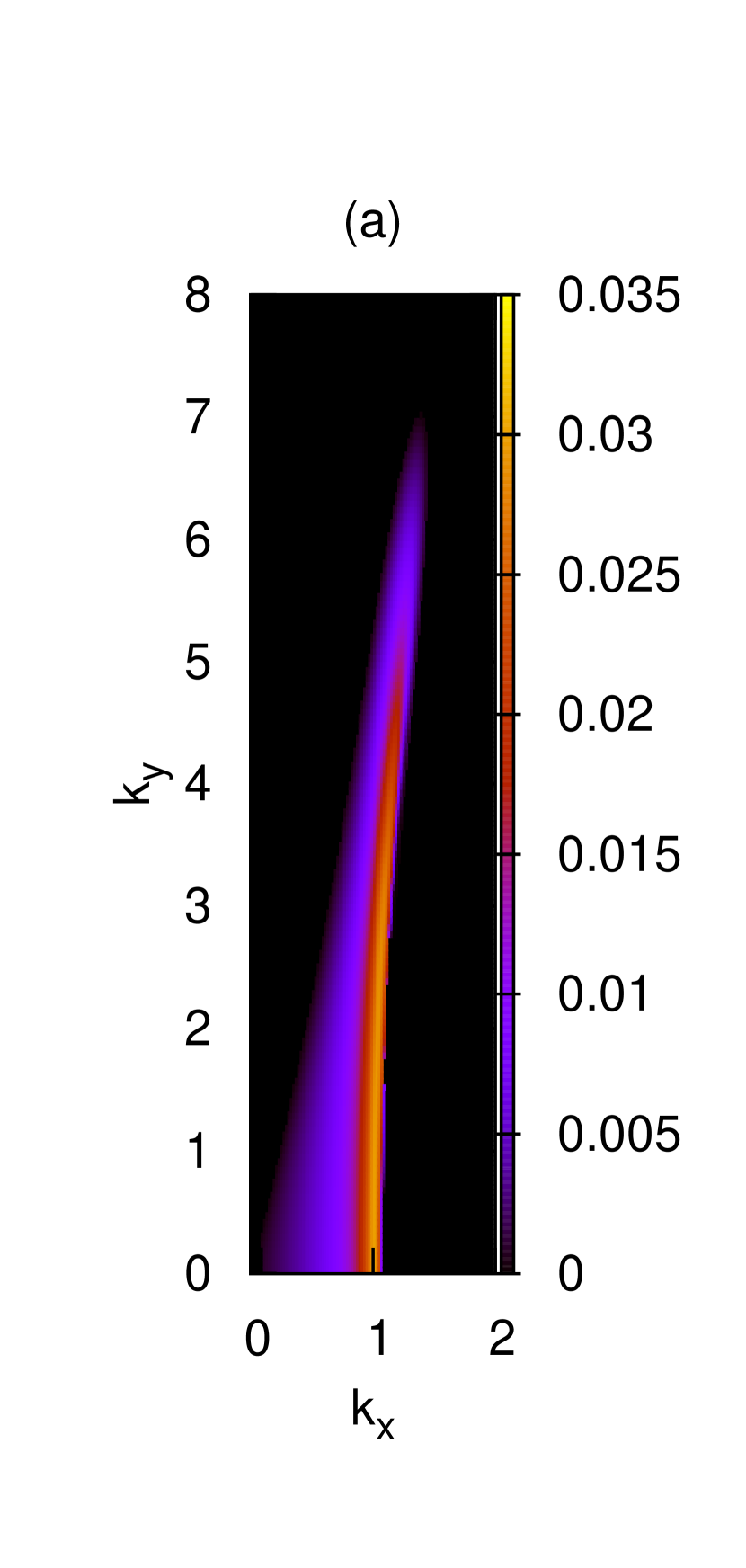
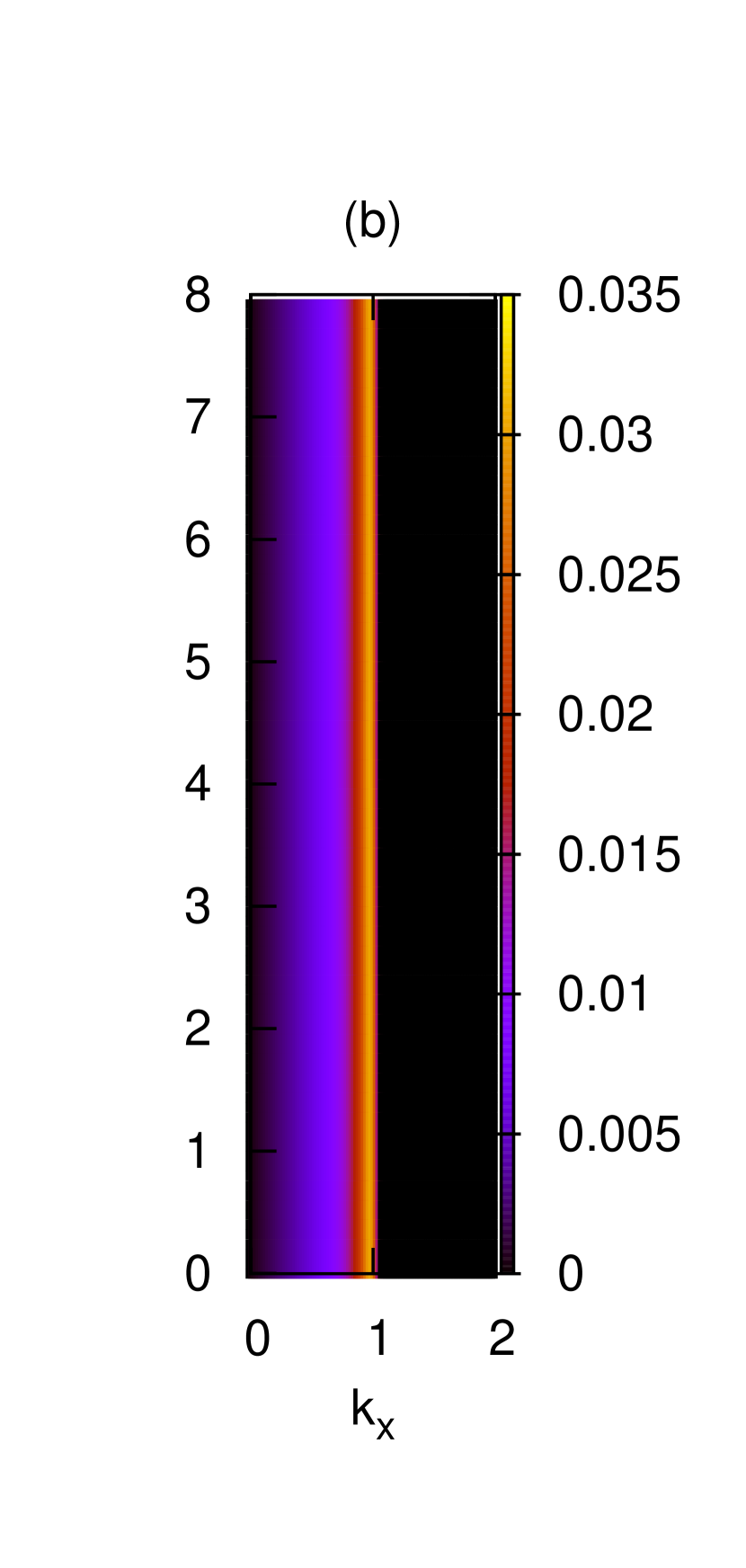
Figure 1: The color contour plot of the growth rate of the Buneman instabilitiy. The left panel (a) is for $v_{\rm d}/v_{\rm th,e}=10,T_{\rm e}=T_{\rm p}$, while the right panel (b) is for the cold limit.

The growth rate obtained by solving the linear dispersion relation is displayed in Figure 1(a). In this condition, the most unstable mode is the Buneman instability. The Buneman instability is caused by the resonance between the electron plasma oscillation of the upstream electrons and proton plasma oscillation of the reflected proton beam. In Figure 1, $k_{x}$ and $k_{y}$ are wavenumbers normalized by $\omega_{\rm pe}/v_{\rm d}$ and the color contours show the growth rate normalized by $\omega_{\rm pe}$, where only the growth rate of growing modes is shown. As is seen, the growth rate of obliquely propagating modes is as large as that of modes parallel to the beam direction. This feature of the Buneman instability can be well understood in the cold limit. We present the results of the cold limit for which all temperatures are set to zero in Figure 1(b). In the cold limit, the distribution function (4) becomes

$$f_{\rm s0}=\delta(v_{x}-v_{\rm d,s})\delta(v_{y}),$$ (9)

and the dispersion relation (2) is reduced to

$$1-\sum_{\rm s}\left(\frac{\omega_{\rm ps}}{\omega-k_{x}v_{\rm d,s}}\right)^{2}=0.$$ (10)

Because $k_{y}$ does not appear in equation (10), the growth rate of electrostatic instabilities in the cold limit does not depend on $k_{y}$. Therefore, in the cold limit, excited waves have any $k_{y}$ and the structure of electrostatic potential to the $y$-direction is strongly disordered and loses coherence to the $y$ direction. This feature is very important to negate the electron surfing acceleration mechanism (Ohira & Takahara, 2007). The maximum growth rate of the Buneman instability in the cold limit is (Buneman, 1958)

$$\gamma_{\rm max}=\left[\frac{3\sqrt{3}}{16}\left(\frac{m_{\rm e}}{m_{\rm p}}\right)\left(\frac{n_{\rm ref}}{n_{\rm e}}\right)\right]^{1/3}\omega_{\rm pe}\ \ {\rm at}\ \ k_{x}=\frac{\omega_{\rm pe}}{v_{\rm d}}=k_{\rm Bun}.$$

In reality, because of a finite temperature, the modes with large wavenumbers are suppressed to grow. This is seen in Figure 1(a); the growth rate for large $k_{y}$ decreases. The dispersion relation of the Buneman instability depends on $v_{\rm th,e}/v_{\rm d}$ and the number density ratio. When $v_{\rm th,e}/v_{\rm d}$ is small, modes that have a large $k_{y}$ can grow as long as the wavelength is larger than the electron Debye length. The wavenumber corresponding to the electron Debye length is $k_{\rm D,e}=\omega_{\rm pe}/v_{\rm th,e}=10k_{\rm Bun}$ in the present plasma condition and the boundary between growing and damping region in Figure 1(a) is about $k_{y}=7k_{\rm Bun}\sim k_{\rm D,e}$, as is consistent with the present consideration. This result implies that in SNRs condition, oblique modes propagating to the beam direction, i.e., to the shock normal, can grow as strongly as the modes to the parallel direction. Because these modes are electrostatic, the direction of the excited electric fields is to the wave vector and the energy density of the electric field of the $y$-component can be larger than that of the $x$-component.

2.2 Ion two-stream instability and ion acoustic instability

After the upstream electrons are heated by the Buneman instability, the thermal velocity of electrons increases up to $v_{\rm th,e}\sim v_{\rm d}$ while the thermal velocity of protons is roughly the same as the initial one, so that the situation of $T_{\rm e}\gg T_{\rm p}$ is realized. The other parameters are the same as in the low temperature case described in the previous subsection. In this condition, while the Buneman instability is stabilized, other types of instabilities can occur. We found that in addition to the ion acoustic instability discussed previously (Cargill & Papadopoulos, 1988), the ion two-stream instability that has not been well noticed in the literature becomes unstable. The ion two-stream instability is caused by the resonance of the ion plasma oscillation of the upstream plasma and that of reflected ions in the situation $T_{\rm e}\gg T_{\rm p}$. Thus, it occurs concurrently with the ion acoustic instability which is caused by the resonance between ion acoustic waves of the reflected protons and electron plasma oscillation of the upstream plasma, where the former modes are mediated by the presence of the hot upstream electrons.

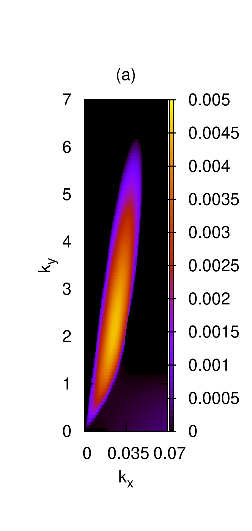
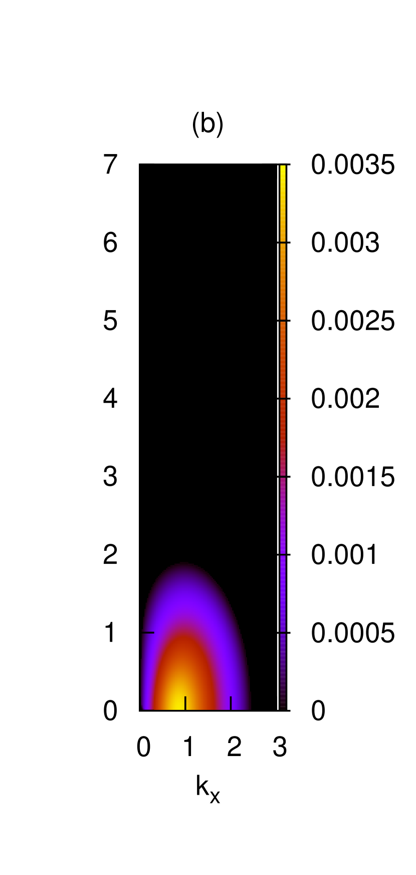
Figure 2: The color contour plot of the growth rate of the ion two-stream instability (the left panel (a)) and that of the ion acoustic instability, for $v_{\rm d}/v_{\rm th,e}=1,T_{\rm e}=100T_{\rm p}$. Note the diffenence in the scale of the abscissa between (a) and (b).

The numerical results of the growth rate for ion two-stream instability and ion acoustic instability are shown in Figures 2(a) and (b), respectively. In Figure 2, $k_{x}$, $k_{y}$ and the growth rate are normalized in the same way as in Figure 1, and the color contours show the growth rate of the growing modes. Note that the difference of the range of the wavenumber in the $x$-direction $k_{x}$ between (a) and (b). While ion acoustic instability grows at around $k_{x}\approx\omega_{\rm pe}/v_{\rm d}$, ion two-stream instabily grows at much smaller $k_{y}$. It is also noted that ion two-stream instability is seen for low but finite values of $k_{y}$, In the present conditions, the wavenumber corresponding to the ion Debye length is $k_{\rm D,p}=\omega_{\rm pi}/v_{\rm th,i}=10k_{\rm Bun}$ while that to the electron Debye length is $k_{\rm Bun}$. Ion plasma oscillation exists between these two wavenumbers. For wavenumbers lower than $k_{\rm Bun}$, it reduces to the ion acoustic mode while for wavenumbers higher than $k_{\rm D,p}$ it damps by thermal motions of ions. It should be noted that in Figure 2(a), ion two-stream modes of parallel propagation to the beam direction are only weakly growing, but that highly oblique modes grow very fast and the maximum growth rate is larger than that of the ion acoustic instability by a factor of a few. The reason is explained as follows. To excite the ion two-stream instability, the resonance condition, $k_{x}v_{\rm d}\sim\omega_{\rm pi}$ must be satisfied in addition to the wavenumber condition mentioned above. The resonance condition requires a small $k_{x}\approx(m_{\rm e}/m_{\rm p})^{1/2}k_{\rm Bun}$. For propagation parallel to the beam direction, this is imcompatible with the wavenumber condition and the growth rate is very small. In contrast, when the wave has a large $k_{y}$, both the wavenumber condition and the resonance condition are fulfilled simultaneously and a larger growth rate is obtained. The results shown in Figure 2 (a) are fully consistent with this picture of the ion two-stream instability.

To understand the ion two-stream instability through the dispersion relation, we consider a situation where the proton temperature is zero and the electron temperature is very high and $k_{y}\gg k_{x}$ (if the electron drift velocity is much smaller than thermal velocity, we do not need the final condition). Then, we can approximate as $|\xi_{\rm p}|,|\xi_{\rm ref}|\gg 1$ and $|\xi_{\rm e}|\ll 1$, and the dispersion relation becomes

$$1+2\left(\frac{k_{\rm D,e}}{k}\right)^{2}-\left(\frac{\omega_{\rm pp}}{\omega}\right)^{2}-\left(\frac{\omega_{\rm ref}}{\omega-k_{x}v_{\rm d,ref}}\right)^{2}=0.$$ (11)

The second term represents the Debye shielding effect of hot electrons and becomes small for $k\gg k_{\rm D,e}$ as discussed above. It is seen that for $k\gg k_{\rm D,e}$, the dispersion relation has the same form as equation (10) and we obtain the maximum growth rate of the ion two-stream instability when $n_{\rm ref}\ll n_{\rm p}$, by replacing $\omega_{\rm pe}$ with $\omega_{\rm pp}$ in equation (11), as

$$\gamma_{\rm max}=\left[\frac{3\sqrt{3}}{16}\left(\frac{n_{\rm ref}}{n_{\rm p}}\right)\right]^{1/3}\omega_{\rm pp}\\ {\rm at}\ \ k_{x}=\frac{\omega_{\rm pp}}{v_{\rm d}}.$$

Because the upstream plasma stays in foot region by about the proton gyro-period $\Omega_{\rm cp}^{-1}$ and because $\Omega_{\rm cp}/\omega_{\rm pp}\sim 4.3\times 10^{-5}$, ion two-stream instability can grow enough in the foot region.

As far as we are aware, this oblique unstable mode has not been considered up to now. We expect that this instability heats ions and that much affects subsequent electron heating processes.

3 Simulation

To perform two-dimensional simulations with real proton electron mass ratio, we confine our attention to the foot region through a proper modeling instead of solving the whole shock structure. Our simulation box is taken to be at rest in the upstream frame of reference, i.e., that of incident protons and electrons. We do not solve electromagnetic waves and concentrate on electrostatic waves.

3.1 Setting

We define the $x$-direction as the shock normal pointing to the shock front, and thus the reflected protons move in the $-x$-direction and returning protons move in the $x$-direction. The magnetic field is taken to be spatially homogeneous pointing in the $z$-direction and we solve the particle motion and electric field in the $x-y$ plane. As the initial condition, we prepare upstream electrons, upstream protons, reflected protons and returning protons. Each population is uniformly distributed in the $x-y$ plane and their momentum distribution is given by a Maxwellian at the same temperatures $T=T_{\rm e}=T_{\rm p}=T_{\rm ref}=T_{\rm ret}=1.75{\rm eV}$. In addition, reflected and returning protons have an extra drift velocity in the $x$-direction of $v_{\rm d}=\pm 0.04c$ ($v_{\rm d}=2v_{\rm sh}$). The number densities of each population are taken as $n_{\rm e}=1.5n_{\rm p}=1\rm{cm}^{-3}$ and $n_{\rm ref}=n_{\rm ret}=0.25n_{\rm p}$, where subscripts e, p, ref and ret represent upstream electrons, upstream protons, reflected protons and returning protons, respectively (see Figure 3). These parameters are typical of young SNRs and satisfy the charge neutrality and a vanishing current.

We employ the periodic boundary condition both in the $x$- and $y$-directions. The electric field is solved by the Poisson equation. We have examined two cases of the background magnetic field, 0 and 90 $\mu$G ($\Omega_{\rm ce}/\omega_{\rm pe}=0$ and 0.03), where $\Omega_{\rm ce}=eB/m_{\rm e}c$ is the electron cyclotron frequency. We sometimes refer the former and latter cases to the unmagnetized and magnetized cases, respectively.

The size of the simulation box to the $x$- and $y$-directions is taken to be $L_{x}=64\lambda_{\rm Bun}$ and $L_{y}=16\lambda_{\rm Bun}$, with a total of 2048 $\times$ 512 cells, where $\lambda_{\rm Bun}=2\pi\omega_{\rm pe}/v_{\rm d}$ is the wavelength of the most unstable mode of the Buneman instability. Thus, the length of each cell $\Delta x=\Delta y$ is 3 times the initial electron Debye length. The number of macroparticles is taken so that initially each cell includes 96 electrons and 96 total protons. The time step $\Delta t$ is taken as $5\times 10^{-3}\omega_{\rm pe}^{-1}$ and the simulation is followed until $3\times 10^{3}\omega_{\rm pe}^{-1}$ or $1.6\times 10^{-3}\Omega_{\rm cp}^{-1}$ where $\Omega_{\rm cp}^{-1}$ corresponds to the time scale the upstream plasma stays in the foot region.

The differences from previous simulations (Ohira & Takahara, 2007) are as follows. First, the initial temperature is lower than the previous one $7{\rm eV}$. This is a more realistic one because the typical temperature of the interstellar matter is about 1eV. Secondly, we add returning proton beam in order that the total current vanishes, although in the electrostatic simulation it is not so critical. Thirdly, simulation time and simulation box are larger than the previous values so that we can investigate the ion two-stream instability.

3.2 Results

Although we have performed simulations for two cases of the magnetic field strength ($0,90\mu G$), the results turn out to be almost the same. Hence, we present the results of the unmagnetized case and add those of the magnetized case when necessary.

First, we discuss the time development of the electric field. The evolution of the spatially averaged energy density of the electric field is shown in Figure 4. The solid and dashed curves show the $x$- and $y$-components, respectively, and bold and thin curves are unmagnetized and magnetized cases, respectively. In the first stage for $t<250\omega_{\rm pe}^{-1}$, the Buneman instability occurs and the electric field to both directions grow. After they attain peak values, they continue to decay till around $t\approx 10^{3}\omega_{\rm pe}^{-1}$. Then, after $t>10^{3}\omega_{\rm pe}^{-1}$, the $y$-component of the electric field starts to grow again while the $x$-component continues to decay. This feature is due to the ion two-stream instability as discussed below.

It should be noted that in the first stage of the Buneman instability ($0<t<250\omega_{\rm pe}^{-1}$), the $y$-component of electric field is larger than the $x$-component. This is different from our previous result. As discussed in §2, this is because the temperature is lower and the waves with a larger obliqueness grow faster compared with our previous simulation (Ohira & Takahara, 2007). In this stage, only electron temperature has risen up to about $m_{\rm e}v_{\rm d}^{2}$, but the ion temperature little changes (see Figure 5). Here, we define the temperature by the velocity dispersion, $T_{\rm s}\equiv m_{\rm s}\langle(v-\langle v\rangle)^{2}\rangle/2k_{\rm B}$.

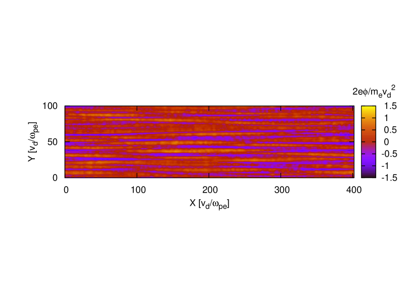
Figure 6: The contour of the electrostatic potential at $t=1740\omega_{\rm pe}^{-1}$.The potential is normalized by $m_{\rm e}v_{\rm d}^{2}/2$. Note that the structure is filamentary so that the electric field is almost perpendicular to the shock normal direction.

In contrast to Cargill & Papadopoulos (1988), after the electrostatic waves caused by the Buneman instability decay at about $t=10^{3}\omega_{\rm pe}^{-1}$, only the $y$-component of the electric field grows and oscillates after the amplitude saturates. In contrast, the $x$-component continues to decay. Of course, this feature can not be seen in one-dimensional simulations. The growth of the $y$-component of electric field is caused by highly oblique ion two-stream instability. If we consider only the parallelly propagating modes as in the one-dimesional simulations, ion acoustic instability has the largest growth rate. In the two-dimensional simulations we can take obliquely propagating modes with $k_{y}\neq 0$ into account, and the growth rate of the ion two-stream instability is larger than that of the ion acoustic instability as mentioned §2. A snapshot of the electrostatic potential at the saturation phase of the ion two-stream instabilities is shown in Figure 6. In Figure 6, spatial coordinates are normalized by $v_{\rm d}/\omega_{\rm pe}$, and the color contours show the electrostatic potential normalized by $m_{\rm e}v_{\rm d}^{2}/2$. Typical wave length scale to the $x$-direction is the order of the resonance scale $2\pi v_{\rm d}/\omega_{\rm pi}$ and that to the $y$-direction is comparable to $2\pi/k_{\rm D,e}$ as the linear analysis predicts. Before the saturation stage, the wavelength is smaller than $2\pi$ electron Debye length for which the linear growth rate is higher.

Time development of the temperatures is shown in Figure 5. The electron temperature rises rapidly up to about $m_{\rm e}v_{\rm d}^{2}$ when the Buneman instability grows, while at this phase the proton temperature does not rise so much. At about $t=10^{3}\omega_{\rm pe}^{-1}$, the proton temperature begins to rise by the growth of the ion two-stream instability but the electron temperature is kept at almost the same because this instability occurs between two ion beams and the energy density of the electric field is nearly 100 times smaller than the thermal energy density of electrons at this stage. At the end of the simulation, upstream proton temperature becomes about 100 times larger than the initial value and the electron to proton temperature ratio $T_{\rm e}/T_{\rm p}$ becomes about 10. For the magnetized case, $T_{\rm e}/T_{\rm p}$ becomes about 7. Although it is not explicitly shown in this paper, the proton distribution has a large anisotropy. Only the proton temperature of the $y$-direction rises up, but that of the $x$-direction is kept to be almost constant.

Figure 7 shows the energy distribution of electrons at the end of the simulation. The bold and thin curves represent non-mangetized and magnetized cases, respectively. It is noted that no high energy tail is seen. Even when there exists a magnetic field, electrons are not accelerated, that is, no surfing acceleration occurs in two-dimensional simulations. Both curves are of a flat top shape and can not be fitted by a Maxwellian distribution. If one draws Maxwellian distribution in Figure 7, it is a straight line with an inclination of $1/k_{\rm B}T_{\rm e}$. As discussed in Ohira & Takahara (2007), at the end of simulation, the electron temperature becomes $T_{\rm e}\sim 0.5m_{\rm e}v_{\rm d}^{2}$. These results are consistent with our previous result (Ohira & Takahara, 2007).

4 Discussion

Now we discuss the final outcome of the ion two-stream instability. It becomes unstable when two conditions are satisfied; one is the resonance condition, $k_{x}v_{\rm d}\sim\omega_{\rm pi}$ and the other is that the wave length be between the ion Debye length and the electron Debye length. Thus, the ion two-stream instability becomes stabilized when $T_{\rm p}\sim T_{\rm e}$. At the end of our simulation, the $y$-component of electric field has not decayed still completely. So, we expect $T_{\rm e}/T_{\rm p}<10$ in the final stage, and probably ions will be heated up to $T_{\rm i}\sim m_{\rm e}v_{\rm d}^{2}\sim 4m_{\rm e}v_{\rm sh}^{2}$ at the foot region in high Mach number perpendicular shocks. Of course, because the proton temperature of the drift direction is still cold in the present simulation, we must check the isotropilazation process of ion velocity distribution by doing longtime full PIC-simulations.

As for the electrons, the electron temperature in the foot region is also about $m_{\rm e}v_{\rm sh}^{2}$. In the later stage, the growth of the two-stream instability dominates over the ion acoustic instability and little electron heating occurs. Hence, as mentioned in Ohira & Takahara (2007), if other electron heating mechanisms do not exist, after passing the shock front, electrons will undergo the adiabatic heating and finally, the electron temperature in the downstream becomes

$$T_{\rm e}\sim 4\times\frac{1}{2}m_{\rm e}(2v_{\rm sh})^{2}=0.41{\rm keV}\left(\frac{v_{\rm sh}}{0.01c}\right)^{2},$$ (12)

where we assume that the compression ratio is 4. This has a very important implication for the electron heating process of the SNR shocks. The proton temperature in the downstream is $T_{\rm p}=3m_{\rm p}v_{\rm sh}^{2}/16$, hence the ratio of two temperatures is

$$T_{\rm e}/T_{\rm p}\sim\frac{128}{3}\frac{m_{\rm e}}{m_{\rm p}}\sim 0.023.$$ (13)

This value is close to the observed value as long as the shock velocity $v_{\rm sh}$ is larger than $1500{\rm km/s}$ (Adelsberg et al., 2008). Namely, we expect that the overheating problem of electrons raised by Cargill & Papadopoulos (1988) can be solved by the ion two-stream instability.

In this paper, we prepare three ion beams as the initial condition. We have also performed simulations for other initial conditions such that there exist upstream electrons, upstream and reflected protons. Electrons and reflected protons have drift velocities to satisfy the vanishing current condition. This situation corresponds to the initial phase of the shock reformation phenomena. The results turn out to be basically the same as those in the results presented in this paper.

Our simulation does not include electromagnetic modes. In the linear stage of the Buneman and ion two-tream instabilities, the effects are negligible because the growth rates of electromagnetic modes are smaller than those of electrostatic modes for $v_{\rm d}\sim 0.01c$. In the nonlinear stage, electromagnetic modes may be important. One of the reasons is that the electrostatic waves with a wave vector almost perpendicular to the drift direction may make currents because the charge fluctuation can not be shielded by electrons in this situation, where the fluctuation scale is smaller than the electron Debye length. Consequently the current may make the magnetic field. It is an interesting speculation that the magnetic field might be amplified more rapidly by the ion two-stream instability than the ion Weibel instability. The other reason is that anisotropic ion heating caused by the highly oblique ion two-stream instability excites the Weibel instability due to ion temperature anisotropy. At the end of our simulations, the ion temperature of $x$-direction is almost the same as initial one and the ratio of the ion temperature of $y$-direction to that of $x$-diretion $T_{\rm iy}/T_{\rm ix}$ is about 100. These two features may lead to magnetic field amplification and accompanying particle acceleration and heating in the shock foot region. We will make full-PIC simulations in future work to investigate these issues.

5 Summary

We performed linear analysis of two-dimensional electrostatic modes and electrostatic two-dimensional PIC simulations with the real proton electron mass ratio to investigate the time evolution of electrostatic waves in the foot region of collisionless shocks with a high Mach number. We consider only the foot region by properly modeling the effects of reflected and returning protons. Performing the linear analysis, we have shown that after electrons are heated by the Buneman instability, the fastest growing mode is not the ion acoustic instability but the highly oblique ion two-stream instability. The latter mode, which has not been noticed previously, is excited by the resonace between ion plasma oscillations of the two proton beams when the electron temperature is much higher than the ion temperature. The PIC simulation confirms that the excitaion of the ion two-stream instability occurs faster than the ion acoustic instability and that protons are heated preferentially to the perpendicular direction to the shock normal direction. As a result, electron heating basically stops at the stage of the Buneman instability and the expected electron temperature in supernova remnants is fully compatible with the observation, avoiding the overheating problem raised by Cargill & Papadopoulos (1988).

Figure 3: The particle distribution in the initial state for the simulation. Solid and dashed curves represent electron and ion distribution functions of $v_{x}$, respectively.

Figure 4: The development of the energy density of electric field. The bold and thin lines represent non-magnetized and magnetized cases, respectively. Solid and dashed curves represent $E_{x}$ and $E_{y}$, respectively.

Figure 5: Time development of the temperatures. The bold and thin lines represent non-magnetized and magnetized cases, respectively. Solid and dashed curves represent electron and proton temperatures, respectively. Dotted curves represent electron proton temperature ratio.

Figure 7: Energy distribution function of electrons at the end of simulations. Bold and thin curves represent non-magnetized and magnetized cases, respectively.

References

- Adelsberg et al. (2008) Adelsberg, M., Heng, K., McCray, R., & Raymond, J. C. 2008, astro-ph/0803.2521
- Bludman et al (1960) Bludman, S. A., Watson, K. M., & Rosenbluth, M. N. 1960, Phys. Fluids, 3, 747
- Buneman (1958) Buneman, O. 1958, Phys. Rev. Lett., 1, 8
- Cargill & Papadopoulos (1988) Cargill, P. J., & Papadopoulos, K. 1988, ApJ, 329, L29
- Hoshino & Shimada (2002) Hoshino, M & Shimada, N. 2002, ApJ, 572, 880
- Koyama et al. (1995) Koyama, K., Petre, R., Gotthelf, E. V., Hwang, U., Matsuura, M., Ozaki, M., & Holt, S. S. 1995, Nature, 378, 225
- Lampe et al. (1974) Lampe, M., Haber, I., Orens, J. H., & Boris, P. 1974, Phys. Fluids, 17, 428
- Leroy (1983) Leroy, M. M. 1983, Phys. Fluids, 26, 2742
- Ohira & Takahara (2007) Ohira, Y., & Takahara, F. 2007, ApJ, 661, L171
- Papadopoulos (1988) Papadopoulos, K. 1988, Ap&SS, 144, 535
- Shimada & Hoshino (2000) Shimada, N., & Hoshino, M. 2000, ApJ, 543, L67
- Stage et al. (2006) Stage, M. D., Allen, F. E., Houck, J. C., & Davis, J. E. Nature Phys., 2, 614
- Watanabe (1991) Watanabe, T. 1991, National Institute for Fusion Science, Nagoya, 65, 556