Abstract

We consider the possibility that there may be causality violation detectable at higher energies. We take a scalar nonlocal theory containing a mass scale $\Lambda$ as a model example and make a preliminary study of how the causality violation can be observed. We show how to formulate an observable whose detection would signal causality violation. We study the range of energies (relative to $\Lambda$) and couplings to which the observable can be used.

1 introduction

Non-local quantum field theories (NLQFT) have been a subject of wide research since 1950’s. The main reason for the interest in early days has been the hope that the non-local quantum field theory can provide a solution to the puzzling aspects of renormalization. The basic idea was that since the divergences in a local quantum filed theory arise from product of fields at identical space-time point, the divergences of the local quantum field theory would be tamed if the interaction were non-local. In particular, if the interaction scale was typically of the order of $1/\Lambda$, then momenta in loop integrals (Euclidean) would be damped when $|p^{2}|>>\Lambda^{2}$. The early work on NLQFT, starting from that by Pais and Uhlenbeck [1] and especially that of Efimov and coworkers, has been summarized in [3]. NLQFT’s also have found application towards description of extended particles which incorporates the symmetries of the theory in some (non-local) form [4]. The non-commutative fields theories, currently being studied [5], are a special variant of a NLQFT, as is evident especially in its QFT representation using the star product. In this work, we shall focus our attention on the type of NLQFT’s formulated by Kleppe and Woodard [6]. One of the reasons we normally insist on a local quantum field theory is because it has micro-causality, and this generally ensures causality of the theory. One of the consequences, therefore, that would be suspected of non-locality would be a causality violation at the level of the S-matrix. Indeed, since at a given moment, the interaction is spread over a finite region in space, thus covering simultaneously space-like separated points, we expect the interaction to induce non-causality. In view of the fact that we have not observed large-scale causality violation, it becomes important to distinguish between theories exhibiting classical violations of causality versus quantum violations of causality. As argued in [2], a violation of causality at the classical level can have a larger effective range and strength, compared to the quantum violations of causality which are suppressed by  $g^{2}/16\pi^{2}$ per loop. We do not know of large scale causality violations, and as such, it is desirable that the non-local theory has no classical violation of causality. One way known to ensure that there is no classical level of causality violation is to require that the S-matrix of the NLQFT at the tree level coincides with that of the local theory ($\Lambda\rightarrow\infty$) as is arranged in the formulation of [6]. We shall work in the context of the NLQFT’s as formulated by Kleppe and Woodard [6]. This form of non-local QFT was evolved out of earlier work of Moffat [4], insights into structure of non-local field equations by Eliezer and Woodard [7] and application to QED by Evens et al [8]. This formulation has a distinct advantage over earlier attempts in several ways:

1. There are no additional classical solutions to the non-local field equations compared to the local ones. The nonlocal theory is truly a deformation of the local theory and the meaning of quantization, as a perturbation about the classical, is not altered. This property is not shared by non-commutative field theories.

2. It has the same S-matrix at the tree level, and thus;

3. There is no classical violation of causality.

4. The theory, unlike a higher derivative theory, has no ghosts and is unitary at a finite $\Lambda$.

5. The theory can embody non-localized versions of local symmetries having an equivalent set of consequences.

There are many other reasons for taking interest in these NLQFT’s. We have found such a non-local formulation with a finite $\Lambda$, very useful in understanding the renormalization program in the renormalizable field theories [9]. We have shown that this formulation enables one to construct a mathematically consistent framework in which the renormalization program can be understood in a natural manner. The framework does not require any violations of mathematical rigor usually associated with the renormalization program. This framework, moreover, made it possible to theoretically estimate the mass scale $\Lambda$. The nonlocal formulations can also be understood [10] as an effective field theory formulation of a physical theory that is valid up to mass scale $\sim$$\Lambda$. In such a case, the unknown physics at energy scales higher than $\Lambda$ [such as a structure in terms of finer constituents, additional particles, forces, supersymmetry etc ] can effectively be represented in a consistent way (a unitary, gauge-invariant, finite (or renormalizable) theory) by the non-local theory. In other words, the nonlocal standard model can serve as such an effective field theory [10] and will afford a model-independent way of consistently reparametrizing the effects beyond standard model. It can be looked upon in a number of other ways. One could think the non-locality as representing a form factor with a momentum cut-off $\Lambda$[4]. One could also think of this theory as embodying a granularity of space-time of the scale $1/\Lambda$ or as an intrinsic mass scale $\Lambda$ [6, 11, 9].
A possible "limitation" of the theory is that the theory necessarily has quantum violations of causality [6, 12]; though it can be interpreted as a prediction of the theory. In another work, A. Jain and one of us explored the question with the help of the simple calculations for the simplest field theory: the nonlocal version of the $\lambda\phi^{4}$ theory [13]. While, in this scalar field model, the causality violation is related to the nonlocality of interaction put in by hand, so to speak, in practice such a non-locality of interaction could arise from many possible sources. It could arise from a fundamental length, $1/\Lambda$, present in nature. It could arise from composite nature of elementary particles (This possibility has recently been explored [14]). In this work, we wish to formulate how the effect can be observed experimentally. In order to study causality violation (CV) in the theory, it is first necessary to formulate quantities that signal CV. We would like to construct quantities that can be measured experimentally. From this view-point, it is appropriate to construct quantities in terms of the S-operator. Bogoliubov and Shirkov [15] have formulated a necessary condition for causality to be preserved in particle physics by the S-operator . This formulation is simple and at the same time extremely general in that, it uses only (i) the phenomenologically accessible S-operator together with (ii) the most basic notion of causality in a relativistic formulation: A cause at $x$ shall not affect physics at any point $y$ unless $y$ is in the forward light-cone with respect to $x$. The condition is formulated as,

$$\begin{array}[]{ccc}\frac{\delta}{\delta g(x)}\left(\frac{\delta S[g]}{\delta g(y)}S^{\dagger}[g]\right)=0&for&x<\sim y\end{array}$$ (1)

where $x<\sim y$ means that either $x^{0}<y^{0}$ or $x$ and $y$ are space like separated. [In either case, there exists a frame in which $x^{0}<y^{0}$]. Section 2 gives a brief qualitative understanding of this relation and how amplitudes indicating causality violation are constructed using this relation. In section 2, we shall also summarize the essentials of construction of a non-local QFT given a local one. In this section, we shall give the results for the exclusive processes $\phi+\phi\rightarrow\phi+\phi$ in the one loop order from [13]. In section 3, we make a comparison of the local contribution and the non-local CV effects and the latter could be significant for $s\leq\Lambda^{2}$ and when one analyzes angular distributions. In section 4, we shall construct a physical observable in terms of a differential cross-section $\frac{d\sigma}{d\Omega}$. This quantity involves some higher order terms and in section 6, we shall make an estimate of them and show that under certain conditions on coupling constant and energies they are indeed negligible and allow observation of the observable constructed in section 3.

While, what we have presented for simplicity, is a model calculation, similar attempt can be made for a more realistic process in the standard model. A work, along the same lines, but applicable to the realistic cases of experimentally observed exclusive processes $e^{+}e^{-}\rightarrow e^{+}e^{-}$,$e^{+}e^{-}\rightarrow\mu^{+}\mu^{-}$and $e^{+}e^{-}\rightarrow\tau^{+}\tau^{-}$ is in progress.

2 preliminary

In this section, we shall briefly discuss the construction of non-local field theories and the Bogoliubov-Shirkov criterion of causality. We shall further summarize results on causality violation calculation in [13, 2].

2.1 non-local quantum field theory

We shall present the construction of the NLQFT as presented in [6]. We start with the local action for a field theory, in terms of a generic field $\phi$, as the sum of the quadratic and the interaction part:

$$S[\phi]=F[\phi]+I[\phi]$$

and express the quadratic piece as

$$F[\phi]=\int d^{4}x\phi_{i}(x)\Im_{ij}\phi_{j}(x)$$

We define the regularized action in terms of the smeared field $\widehat{\phi}$, defined in terms of the kinetic energy operator $\Im_{ij}$ as,

$$\widehat{\phi}\equiv\mathcal{E}^{-1}\phi\,\,\,\,\,\,\,\,\,\,\,\mathcal{E}\equiv\exp[\Im/\Lambda^{2}]$$

The nonlocally regularized action is constructed by first introducing an auxiliary action $S[\phi,\psi]$. It is given by

$$S[\phi,\psi]=F[\hat{\phi}]-A[\psi]+I[\phi+\psi]$$

where $\psi$ is called a “shadow field” with an action

$$A[\psi]=\int d^{4}x\psi_{i}O_{ij}^{-1}\psi_{j};\;\;O\equiv\frac{\mathcal{E}^{2}-1}{\Im}$$

The action of the non-local theory is defined as $\hat{S}[\phi]=S[\phi,\psi]\|_{{}_{\psi=\psi[\phi]}}$ where $\psi[\phi]$ is the solution of the classical equation $\frac{\delta S}{\delta\psi}=0$.
The vertices are unchanged but every leg can connect either to a smeared propagator

$$\frac{i\mathcal{E}^{2}}{\Im+i\epsilon}=-i\int_{1}^{\infty}\frac{d\tau}{\Lambda^{2}}exp\{\frac{\Im\tau}{\Lambda^{2}}\}$$

or to a shadow propagator [shown by a line crossed by a bar]

$$\frac{i[1-\mathcal{E}^{2}]}{\Im+i\epsilon}=-iO=-i\int_{0}^{1}\frac{d\tau}{\Lambda^{2}}exp\{\frac{\Im\tau}{\Lambda^{2}}\}$$

In the context of the $\lambda\phi^{4}$ theory, we have,

$$\Im=-\partial^{2}-m^{2}\quad I(\phi)=-\frac{g}{4}\phi^{4}$$

We shall now make elaborative comments. The procedure constructs an action having an infinite number of terms (each individually local), and having arbitrary order derivatives of $\phi$. The net result is to give convergence in the Euclidean momentum space beyond a momentum scale $\Lambda$ through a factor of the form $\exp{(\frac{p^{2}-m^{2}}{\Lambda^{2}})}$ in propagators. The construction is such that there is a one-to-one correspondence between the solutions of the local and the non-local classical field equations, (a difficult task indeed [7]). It can also be made to preserve the local symmetries of the local action in a non-localized form [6]. The Feynman rules for the scalar nonlocal theory are simple extensions of the local ones. In momentum space, these read:

1. For the $\phi$-propagator (smeared propagator) denoted by a straight line:

   $$i\frac{exp\left[\frac{p^{2}-m^{2}+i\epsilon}{\Lambda^{2}}\right]}{p^{2}-m^{2}+i\epsilon}=\frac{-i}{\Lambda^{2}}\int_{1}^{\infty}d\tau\exp\left\{\tau\left[\frac{p^{2}-m^{2}+i\epsilon}{\Lambda^{2}}\right]\right\}$$

2. For the $\psi$-propagator denoted by a barred line:

   $$i\frac{1-exp\left[\frac{p^{2}-m^{2}+i\epsilon}{\Lambda^{2}}\right]}{p^{2}-m^{2}+i\epsilon}=\frac{-i}{\Lambda^{2}}\int_{0}^{1}d\tau\exp\left\{\tau\left[\frac{p^{2}-m^{2}+i\epsilon}{\Lambda^{2}}\right]\right\}$$

3. The 4-point vertex is as in the local theory, except that any of the lines emerging from it can be of either type. (There is accordingly a statistical factor).

4. In a Feynman diagram, the internal lines can be either shadow or smeared, with the exception that no diagrams can have closed shadow loops.

Lower bound has been put on the scale of non-locality $\Lambda$[11, 18] from $g-2$ of muon and precision tests of standard model. It has been argued that an upper bound on the scale $\Lambda$ can be obtained from the requirement that renormalization program is naturally understood in a nonlocal field theory setting [9, 10]. Should particles of standard model be composite, $\Lambda$ could naturally be related to the compositeness scale [14].

2.2 bogoliubov-shirkov causality criterion

The causality condition that we have used to investigate causality violation in NLQFT is the one discussed by Bogoliubov and Shirkov [15]. They have shown that an S-matrix for a theory that preserves causality must satisfy the condition of Eq.(2)

$$\frac{\delta}{{\delta g(x)}}\left({\frac{{\delta S(g)}}{{\delta g(y)}}S^{\dagger}(g)}\right)=0~{}for~{}x<\sim y$$ (2)

and it has been formulated treating the coupling $g(x)$ as space-time dependent. A simple qualitative understanding can be provided as in [2]. The above relation is a series in $g(x)$ and leads perturbatively to an infinite set of equations when expanded using

$$S[g]=1+\sum_{n\geq 1}\frac{1}{n!}\int S_{n}(x_{1},...,x_{n})g(x_{1})...g(x_{n})dx_{1}...dx_{n}.$$ (3)

We consider the following expression

$$H(y;g) = i\frac{{\delta S(g)}}{{\delta g(y)}}S^{\dagger}(g)$$

$$= \sum\limits_{n\geq 0}{\frac{1}{{n!}}}\int{H_{n}(y,x_{1},...x_{n})g(x_{1})...g(x_{n})dx_{1}...dx_{n}}$$

We shall write only a few of each of these coefficient functions

$$H_{1}(x,y)\equiv iS_{2}(x,y)+iS_{1}(x)S_{1}^{\dagger}(y)$$ (4)

$$H_{2}(x,y,z)\equiv iS_{3}(x,y,z)+iS_{1}(x)S_{2}^{\dagger}(y,z)+iS_{2}(x,y)S_{1}^{\dagger}(z)+iS_{2}(x,z)S_{1}^{\dagger}(y)$$ (5)

(for a general expression for $H_{n}$, see [13]). Then, the causality condition (2) reads,

$$\frac{\delta}{{\delta g(x)}}H\left(y,g\right)=0\qquad for\;x<\sim y$$

which implies,

$$H_{1}\left(x,y\right)=0\qquad y<\sim x$$ (6)

$$H_{2}\left(x,y,z\right)=0\qquad y<\sim x\,\mbox{and/or}\,z<\sim x$$ (7)

if causality is to be preserved. These quantities can be further simplified by the use of unitarity relation $S^{\dagger}(x)S(x)=\mathcal{I}$, expanded similarly in powers of $g(x)$.
These are given by

$$S_{1}(x)+S_{1}^{\dagger}(x)=0$$ (8)

$$S_{2}(x,y)+S_{2}^{\dagger}(x,y)+S_{1}(x)S_{1}^{\dagger}(y)+S_{1}(y)S_{1}^{\dagger}(x)=0$$ (9)

In the case of the local theory, these causality relations [(6) and (7)] are trivially satisfied. In the case of the nonlocal theories, such quantities, on the other hand, afford a way of characterizing the causality violation. However, these quantities contain not the usual S-matrix elements that one can observe in an experiment (which are obtained with a constant i.e. space-time-independent coupling), but rather the coefficients in (3). We thus find it profitable to construct appropriate space-time integrated versions out of $H_{n}(y,x_{1},...,x_{n})$. Thus, for example, we can consider

$$H_{1} \equiv \int d^{4}x\int d^{4}y[\vartheta(x_{0}-y_{0})H_{1}(x,y)+\vartheta(y_{0}-x_{0})H_{1}(y,x)]$$ (10)

$$= i\int d^{4}x\int d^{4}yS_{2}(x,y)-i\int d^{4}x\int d^{4}yT[S_{1}(x)S_{1}(y)]$$

which can be expressed entirely in terms of Feynman diagrams that appear in the usual S-matrix amplitudes. In a similar manner, we can formulate

$$H_{2} \equiv \int d^{4}x\int d^{4}y\int d^{4}zH_{2}(x,y,z)\vartheta(x_{0}-y_{0})\vartheta(y_{0}-z_{0})$$ (11)

$$+5\,\mbox{symmetric}\;\mbox{terms}$$

and can itself be expressed in terms of Feynman diagrams.
There is a subtle point regarding the expansion (3) of the S-matrix in terms of coupling $g$. In a field theory, the coupling $g$, which has to be the renormalized one, is not a uniquely defined quantity. In this respect, we have to make a renormalization convention. In view of the fact that CV, if at all observed, is expected to be observed at large energies [13], we prefer to use $g$ renormalized at a large energy scale; since that assures more rapid convergence of the perturbation series. We shall therefore assume that

$$\widetilde{g}=Re\Gamma^{\left(4\right)}\left(s=-2s_{0}+2m^{2},t=u=s_{0}+m^{2}\right)$$

where $s_{0}$ is a large positive number and $\sqrt{s_{0}}\sim$ C.M. energy of collision. Here, $\Gamma^{\left(4\right)}$ is the proper 4-point vertex and $s=-2s_{0}+2m^{2},t=u=s_{0}+m^{2}$ is a point in the unphysical region compatible with $p_{i}^{2}=m^{2}$. This is equivalent to the following convention:

$$Re\Gamma_{\left(n\right)}^{\left(4\right)}\left(s=-2s_{0}+2m^{2},t=u=s_{0}+m^{2}\right)=0;\qquad n=1,2,3,...$$

where $\Gamma_{\left(n\right)}^{\left(4\right)}$ refers to the $n-$loop contribution to $\Gamma^{\left(4\right)}$. The numerical value of $\tilde{g}$ can be determined by comparing the total experimental cross-section with the expression for it upto a desired order.

2.3 Results of [13] about CV

In the reference [13], CV in a nonlocal scalar $\phi^{4}$ theory was studied. It was shown that one can construct amplitudes, which if non-zero, necessarily imply CV. These amplitudes,( $H_{1}$, $H_{2}$ etc of 10 and 11) can moreover be calculated by means of Feynman diagrams. In [13], causality violation in two exclusive processes (i) $\phi\;\phi\rightarrow\phi\;\phi$ and (ii) $\phi\;\phi\rightarrow\phi\;\phi\;\phi\;\phi$ were studied. It was in particular demonstrated that CV grows significantly with $s$. Here, we shall recall only the result for the first process: $\phi\;\phi\rightarrow\phi\;\phi$ As shown in [13], the s-channel diagram for the CV amplitude (in the massless) limit yields (the relevant figure, fig. 1, is found in a future section) the following contribution to the transition amplitude:

$$\Gamma(s)=\frac{{9{\tilde{g}}^{2}}}{{4\pi^{2}}}\sum\limits_{n=0}^{\infty}{\frac{{\left({\frac{s}{{\Lambda^{2}}}}\right)^{n}\left({1-\frac{1}{{2^{n}}}}\right)}}{{n((n+1)!)}}}$$

The net causality violating amplitude, considering all the three $s,t,u$ channels, takes the following form in the massless limit:

$$\Delta M_{nonlocal}(s,t,u)$$ (12)

$$= \frac{{9{\tilde{g}}^{2}}}{{4\pi^{2}}}\sum\limits_{n=0}^{\infty}{\frac{{\left({1-\frac{1}{{2^{n}}}}\right)}}{{n((n+1)!)}}}\left\{{\left({\frac{s}{{\Lambda^{2}}}}\right)^{n}+\left({\frac{t}{{\Lambda^{2}}}}\right)^{n}+\left({\frac{u}{{\Lambda^{2}}}}\right)^{n}}\right\}$$ (13)

This CV amplitude is analytic in $s,t,u$ and $m$.

3 comparison of cv and local contributions

We shall compare the CV terms of (13) of [13] with the usual local amplitude to get a judgment as to how and when the former can be isolated.

3.1 local theory

For the local theory, we find[17]

$$M_{local}=-\frac{{36{\tilde{g}}^{2}}}{{32\pi^{2}}}\left[{\ln s+\ln t+\ln u}+constant\right]=-\frac{{36{\tilde{g}}^{2}}}{{32\pi^{2}}}\ln\left[stu\right]+constant$$

In the center of mass frame the Mandelstam variables are given as follows:

$$s = (k_{1}+k_{2})^{2}=(p_{1}+p_{2})^{2}=4p^{2}+4m^{2}$$

$$t = (k_{1}-p_{1})^{2}=(k_{2}-p_{2})^{2}=-2p^{2}(1-cos\theta)$$

$$u = (k_{1}-p_{2})^{2}=(k_{2}-p_{1})^{2}=-2p^{2}(1+cos\theta)$$

So that

$$M_{local} = -\frac{{36{\tilde{g}}^{2}}}{{32\pi^{2}}}\left[{\ln stu}\right]+constant$$

$$\approx -\frac{{36{\tilde{g}}^{2}}}{{32\pi^{2}}}\left[{\ln\left(16p^{6}(1-\cos^{2}\theta)\right)}\right]+constant$$

(We have ignored $m^{2}$ compared to $s$ at high energies). The amplitude can now be expressed in term of the Legendre polynomials as follows:

$$M_{local} \equiv M_{local}(\cos\theta)$$

$$= \sum\limits_{l=0}^{\infty}{a_{l}^{local}}P_{l}(\cos\theta)$$

Where,

$$a_{l}^{local} = \frac{{2l+1}}{2}\int\limits_{-1}^{+1}{M_{local}(\cos\theta)}P_{l}(\cos\theta)d\cos\theta$$

$$= (-1)^{n}\frac{{2l+1}}{{2^{l+1}l!}}\int\limits_{-1}^{+1}{M_{local}^{n}(x)}\frac{{d^{l-n}}}{{dx^{l-n}}}(x^{2}-1)^{l}dx$$

$$= (-1)^{n+1}\frac{{2l+1}}{{2^{l+1}l!}}\frac{{36{\tilde{g}}^{2}}}{{32\pi^{2}}}\int\limits_{-1}^{+1}{\frac{{d^{n}}}{{dx^{n}}}[\ln(1-x^{2})]}\frac{{d^{l-n}}}{{dx^{l-n}}}(x^{2}-1)^{l}dx$$

Here $M_{local}^{n}(x)$ stands for the $n$-th derivative of $M_{local}(x)$ with respect to its argument. The coefficients $a_{2}^{local},a_{4}^{local},a_{6}^{local}$ are obtained as follows:

$$a_{2}^{local} = (-1)^{1+1}\frac{5}{{2^{3}2!}}\frac{{36{\tilde{g}}^{2}}}{{32\pi^{2}}}\int\limits_{-1}^{+1}{\frac{d}{{dx}}[\ln(1-x^{2})]}\frac{d}{{dx}}(x^{2}-1)^{2}dx=\frac{{36{\tilde{g}}^{2}}}{{32\pi^{2}}}\left({\frac{5}{3}}\right)$$

$$a_{4}^{local} = (-1)^{1+1}\frac{9}{{2^{5}4!}}\frac{{36{\tilde{g}}^{2}}}{{32\pi^{2}}}\int\limits_{-1}^{+1}{\frac{d}{{dx}}[\ln(1-x^{2})]}\frac{{d^{3}}}{{dx^{3}}}(x^{2}-1)^{4}dx=\frac{{36{\tilde{g}}^{2}}}{{32\pi^{2}}}\left({\frac{9}{{10}}}\right)$$

$$a_{6}^{local} = (-1)^{3+1}\frac{{13}}{{2^{7}6!}}\frac{{36{\tilde{g}}^{2}}}{{32\pi^{2}}}\int\limits_{-1}^{+1}{\frac{{d^{3}}}{{dx^{3}}}[\ln(1-x^{2})]}\frac{{d^{3}}}{{dx^{3}}}(x^{2}-1)^{6}dx=\frac{{36{\tilde{g}}^{2}}}{{32\pi^{2}}}\left({\frac{{13}}{{21}}}\right)$$

Therefore, we have

$$M_{local} = \sum\limits_{l=0}^{\infty}{a_{l}^{local}}P_{l}(\cos\theta)=constant+a_{2}^{local}P_{2}(\cos\theta)+a_{4}^{local}P_{4}(\cos\theta)+a_{6}^{local}P_{6}(\cos\theta)+...$$ (14)

$$= \frac{{36{\tilde{g}}^{2}}}{{32\pi^{2}}}\left(constant^{\prime}+\frac{5}{3}P_{2}(\cos\theta)+\frac{9}{{10}}P_{4}(\cos\theta)+\frac{{13}}{{21}}P_{6}(\cos\theta)+....\right)$$

3.2 nonlocal theory : $\phi\phi\to\phi\phi$

As stated earlier, we wish to compare the CV amplitude of [13] with the local amplitude to see how the former can be isolated. As shown in [13], the s-channel diagram for the CV amplitude (in the massless) limit yields the following contribution to the transition amplitude:

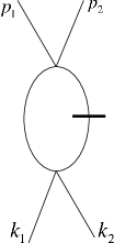
Figure 1: The s-channel diagram giving rise to the one loop causality violating amplitude $H_{1}$.

$$\Gamma(s)=\frac{{9{\tilde{g}}^{2}}}{{4\pi^{2}}}\sum\limits_{n=0}^{\infty}{\frac{{\left({\frac{s}{{\Lambda^{2}}}}\right)^{n}\left({1-\frac{1}{{2^{n}}}}\right)}}{{n((n+1)!)}}}$$

The net causality violating amplitude, considering all the three $s,t,u$ channels, takes the following form in the massless limit:

$$\Delta M_{nonlocal}(s,t,u)$$

$$= \frac{{9{\tilde{g}}^{2}}}{{4\pi^{2}}}\sum\limits_{n=0}^{\infty}{\frac{{\left({1-\frac{1}{{2^{n}}}}\right)}}{{n((n+1)!)}}}\left\{{\left({\frac{s}{{\Lambda^{2}}}}\right)^{n}+\left({\frac{t}{{\Lambda^{2}}}}\right)^{n}+\left({\frac{u}{{\Lambda^{2}}}}\right)^{n}}\right\}$$

In the center of mass frame, we have

$$\Delta M_{nonlocal} = \frac{{9{\tilde{g}}^{2}}}{{4\pi^{2}}}\sum\limits_{n=0}^{\infty}{\frac{{\left({1-\frac{1}{{2^{n}}}}\right)}}{{n((n+1)!)}}\frac{1}{{\Lambda^{2n}}}}\left({(4p^{2})^{n}+(-2p^{2})^{n}\{(1-\cos\theta)^{n}+(1+\cos\theta)^{n}\}}\right)$$

$$= \sum_{l=0}{a_{l}^{nonlocal}}P_{l}(\cos\theta)$$

Comparison of $M_{local}$ and $\Delta M_{nonlocal}$ is facilitated by comparing Legendre coefficients of the same orders. The coefficients $a_{2}^{nonlocal},a_{4}^{nonlocal}$ and $a_{6}^{nonlocal}$ are computed as below:

$$a_{2}^{nonlocal} = \frac{5}{2}\int\limits_{-1}^{+1}{\Delta M_{nonlocal}(\cos\theta)}P_{2}(\cos\theta)d\cos\theta=\frac{{9{\tilde{g}}^{2}}}{{4\pi^{2}}}\left({\frac{{p^{2}}}{{\Lambda^{2}}}}\right)^{2}\frac{1}{3}$$

$$a_{4}^{nonlocal} = \frac{9}{2}\int\limits_{-1}^{+1}{\Delta M_{nonlocal}(\cos\theta)}P_{4}(\cos\theta)d\cos\theta=\frac{{9{\tilde{g}}^{2}}}{{4\pi^{2}}}\left({\frac{{p^{2}}}{{\Lambda^{2}}}}\right)^{4}\frac{1}{{70}}$$

$$a_{6}^{nonlocal} = \frac{{13}}{2}\int\limits_{-1}^{+1}{\Delta M_{nonlocal}(\cos\theta)}P_{6}(\cos\theta)d\cos\theta=\frac{{9{\tilde{g}}^{2}}}{{4\pi^{2}}}\left({\frac{{p^{2}}}{{\Lambda^{2}}}}\right)^{6}\frac{1}{{3465}}$$

We summarize the ratio of the local and nonlocal coefficients and their numerical values in the following table:

Ratio of coefficients	$\frac{p^{2}}{\Lambda^{2}}=0.1$	$\frac{p^{2}}{\Lambda^{2}}=0.2$	$\frac{p^{2}}{\Lambda^{2}}=0.4$	$\frac{p^{2}}{\Lambda^{2}}=0.8$
$\frac{a_{2}^{nonlocal}}{a_{2}^{local}}$	0.4%	1.6%	6.4%	25.6%
$\frac{a_{4}^{nonlocal}}{a_{4}^{local}}$	0.00032%	0.0051%	0.081%	1.3%
$\frac{a_{6}^{nonlocal}}{a_{6}^{local}}$	9.3$\times 10^{-10}$	6$\times 10^{-8}$	3.8$\times 10^{-6}$	2.4$\times 10^{-4}$

Table 1: Comparison of local and non-local contributions for coefficients of different Legendre polynomials.

These ratios are independent of the coupling constant $g$. It appears that there is a significant chance of detecting CV only in the ratio $\frac{a_{2}^{nonlocal}}{a_{2}^{local}}$ and when $p^{2}\lesssim\Lambda^{2}$.
Finally we point out that while we have picked up the process $\phi\phi\rightarrow\phi\phi$ for simplicity, this would not be the process for which observation of CV is the most efficient. This is so because as pointed out in [13], the CV in this process is of higher order in $\frac{p^{2}}{\Lambda^{2}}$, viz. $O\left(\frac{p^{4}}{\Lambda^{4}}\right)$. CV should be more noticeable in a process such as $\phi\phi\rightarrow\phi\phi\phi\phi$.

4 construction of observables

In this section, we shall construct a quantity, partly dependent on physically observable differential cross-section and partly on perturbative calculations, which can detect CV. Of course, we make use of the quantities $H_{1}$ of eq.(10) which signal CV [13, 2]. The S-operator has the expansion:

$$S=1+g\int d^{4}xS_{1}\left(x\right)+\frac{g^{2}}{2!}\int d^{4}xd^{4}yS_{2}\left(x,y\right)+..........$$

Consider a following matrix element between some initial and final states $\left|i\right\rangle$ and $\left|f\right\rangle$:

$$\left\langle f\right|S\left|i\right\rangle=\delta_{fi}+g\int d^{4}x\left\langle f\right|S_{1}\left(x\right)\left|i\right\rangle+\frac{g^{2}}{2!}\int d^{4}xd^{4}y\left\langle f\right|S_{2}\left(x,y\right)\left|i\right\rangle+..........$$

We have, from translational invariance,

$$\int d^{4}x\left\langle f\right|S_{1}\left(x\right)\left|i\right\rangle=\int d^{4}x\left\langle f\right|S_{1}\left(0\right)\left|i\right\rangle e^{i\left(p_{f}-p_{i}\right).x}=\left\langle f\right|S_{1}\left(0\right)\left|i\right\rangle\left(2\pi\right)^{4}\delta^{4}\left(p_{f}-p_{i}\right)$$

Expressing $x=\left(\xi+\eta\right)/2$ and $y=\left(\eta-\xi\right)/2$, we have

$$\int{d^{4}xd^{4}y}\left\langle{f\left|{S_{2}(x,y)}\right|i}\right\rangle = \left(\frac{1}{2}\right)^{4}\int{d^{4}\xi d^{4}\eta}\left\langle{f\left|{S_{2}\left(\frac{{\eta+\xi}}{2},\frac{{\eta-\xi}}{2}\right)}\right|i}\right\rangle$$

$$= \left(\frac{1}{2}\right)^{4}\int{d^{4}\xi d^{4}\eta}\left\langle{f\left|{e^{iP.\frac{\eta}{2}}S_{2}\left(\frac{\xi}{2},-\frac{\xi}{2}\right)e^{-iP.\frac{\eta}{2}}}\right|i}\right\rangle$$

$$= \left(\frac{1}{2}\right)^{4}\int{d^{4}\xi d^{4}\eta}\left\langle{f\left|{e^{ip_{f}.\frac{\eta}{2}}S_{2}\left(\frac{\xi}{2},-\frac{\xi}{2}\right)e^{-ip_{i}.\frac{\eta}{2}}}\right|i}\right\rangle$$

$$= \int{d^{4}\xi}\left\langle{f\left|S_{2}\left(\frac{\xi}{2},-\frac{\xi}{2}\right)\right|i}\right\rangle(2\pi)^{4}\delta^{4}(p_{f}-p_{i})$$

The S-matrix is related to the invariant matrix element $\mathcal{M}_{fi}$ as:

$${\left\langle f\left|S\right|i\right\rangle} \equiv S_{fi} =\left\langle{f|i}\right\rangle+i\left\langle{f\left|T\right|i}\right\rangle$$

$$= \left\langle{f|i}\right\rangle+i(2\pi)^{4}\delta^{4}(p_{f}-p_{i})\mathcal{M}_{fi}$$

Thus,

$$\mathcal{M}_{fi} = -ig\left\langle{f\left|{S_{1}(0)}\right|i}\right\rangle+\frac{{-ig^{2}}}{2}\int{d^{4}\xi}\left\langle{f\left|S_{2}\left(\frac{\xi}{2},-\frac{\xi}{2}\right)\right|i}\right\rangle$$

$$+ \frac{-ig^{3}}{3!}\int d^{4}\xi d^{4}\eta\left\langle{f\left|S_{3}\left(0,\xi,\eta\right)\right|i}\right\rangle+.....$$

$$\equiv \mathcal{M}^{(1)}+\mathcal{M}^{(2)}+\mathcal{M^{\mathit{\mathrm{(3)}}}}+....$$

Now, consider the exclusive scattering process: $\phi\left(k_{1}\right)+\phi\left(k_{2}\right)\rightarrow\phi\left(p_{1}\right)+\phi\left(p_{2}\right)$. The differential cross-section reads:

$$\frac{{d\sigma}}{{d^{3}p_{1}d^{3}p_{2}}}=\frac{1}{2}\frac{{(2\pi)^{4}\delta^{4}(p_{f}-p_{i})}}{{2\omega_{p_{1}}2\omega_{p_{2}}\left|{\vec{v}_{1}-\vec{v}_{2}}\right|2\omega_{k_{1}}2\omega_{k_{2}}}}\left|{\mathcal{M}}\right|^{2}$$

Here, $p_{i}=k_{1}+k_{2}$ and $p_{f}=p_{1}+p_{2}$ and $\mathbf{v_{1,2}}$ are velocities of the colliding particles and $\frac{1}{2}$ is the symmetry factor. [We are using the conventions as outlined in [17]]. We integrate over $p_{2}$ using the $\delta^{3}\left(\mathbf{p_{f}-p_{i}}\right)$. We express $d^{3}p_{1}=p_{1}^{2}dp_{1}d\Omega$, integrate over $p_{1}$ to find,

$$\frac{{d\sigma}}{{d\Omega}}=\int p_{1}^{2}dp_{1}\frac{1}{2}\frac{{(2\pi)^{4}\delta(k_{10}+k_{20}-p_{10}-p_{20})}}{{2\omega_{p_{1}}2\omega_{p_{2}}\left|{\vec{v}_{1}-\vec{v}_{2}}\right|2\omega_{k_{1}}2\omega_{k_{2}}}}\left|{\mathcal{M}}\right|^{2}$$

In the C.M. frame, $k_{10}+k_{20}\equiv 2\sqrt{k^{2}+m^{2}}\equiv 2\omega_{k}$ and $p_{10}+p_{20}\equiv 2\sqrt{p^{2}+m^{2}}=2\omega_{p}$. So that,

$$\frac{{d\sigma}}{{d\Omega}}=\frac{p\omega_{p}}{4}\frac{{(2\pi)^{4}}}{{2\omega_{p_{1}}2\omega_{p_{2}}\left|{\vec{v}_{1}-\vec{v}_{2}}\right|2\omega_{k_{1}}2\omega_{k_{2}}}}\left|{\mathcal{M}}\right|^{2}$$

Here,

$$\left|\mathcal{M}\right|^{2} = \left|{-ig\left\langle{f\left|{S_{1}(0)}\right|i}\right\rangle-i\frac{{g^{2}}}{2}\int{d\xi}\left\langle{f\left|S_{2}\left(\frac{\xi}{2},-\frac{\xi}{2}\right)\right|i}\right\rangle+....}\right|^{2}$$

$$= g^{2}\left|{\left\langle{f\left|{S_{1}(0)}\right|i}\right\rangle}\right|^{2}+g^{3}{\rm Re}\left[{\left\langle{f\left|{S_{1}(0)}\right|i}\right\rangle^{*}\int{d\xi}\left\langle{f\left|S_{2}\left(\frac{\xi}{2},-\frac{\xi}{2}\right)\right|i}\right\rangle}\right]+\mathcal{R}$$

$\mathcal{R}$ are the $O\left(g^{4}\right)$ terms:

$$\mathcal{R} \equiv \frac{g^{4}}{4}\left|\int{d\xi}\left\langle{f\left|S_{2}\left(\frac{\xi}{2},-\frac{\xi}{2}\right)\right|i}\right\rangle\right|^{2}$$ (15)

$$+ 2\frac{g^{4}}{3!}Re\left[\left\langle{f\left|{S_{1}(0)}\right|i}\right\rangle^{*}\int d^{4}\xi d^{4}\eta\left\langle{f\left|S_{3}\left(0,\xi,\eta\right)\right|i}\right\rangle\right]$$

The differential cross-section, now becomes:

$$\frac{{d\sigma}}{{d\Omega}} = \frac{p\omega_{p}}{4}(2\pi)^{4}$$

$$\times \frac{{\left\{{g^{2}\left|{\left\langle{f\left|{S_{1}(0)}\right|i}\right\rangle}\right|^{2}+g^{3}{\rm Re}\left[{\left\langle{f\left|{S_{1}(0)}\right|i}\right\rangle^{*}\int{d\xi}\left\langle{f\left|S_{2}\left(\frac{\xi}{2},-\frac{\xi}{2}\right)\right|i}\right\rangle}\right]+O(g^{4})}\right\}}}{{2\omega_{p_{1}}2\omega_{p_{2}}\left|{\vec{v}_{1}-\vec{v}_{2}}\right|2\omega_{k_{1}}2\omega_{k_{2}}}}$$

Now,

$$iM = g\left\langle{p_{1}p_{2}\left|{S_{1}(0)}\right|k_{1}k_{2}}\right\rangle$$

is the lowest order amplitude which equals $-6ig$. Therefore it is required that

$$\left\langle{p_{1}p_{2}\left|{S_{1}(0)}\right|k_{1}k_{2}}\right\rangle=-6i$$

Thus,

$$\frac{{d\sigma}}{{d\Omega}}$$

$$= \frac{p\omega_{p}}{4}\frac{{(2\pi)^{4}\left\{{36g^{2}-6g^{3}Im\left[\int{d\xi}\left\langle{f\left|S_{2}\left(\frac{\xi}{2},-\frac{\xi}{2}\right)\right|i}\right\rangle\right]+O(g^{4})}\right\}}}{{2\omega_{p_{1}}2\omega_{p_{2}}\left|{\vec{v}_{1}-\vec{v}_{2}}\right|2\omega_{k_{1}}2\omega_{k_{2}}}}$$

and subtracting the angular average of $\frac{{d\sigma}}{{d\Omega}}$

$$\frac{{d\sigma}}{{d\Omega}}-\overline{\frac{{d\sigma}}{{d\Omega}}}$$ (16)

$$= \frac{p\omega_{p}}{4}(2\pi)^{4}$$

$$\times \frac{{\left\{{-6g^{3}Im\left[\int{d\xi}\left\langle{f\left|S_{2}\left(\frac{\xi}{2},-\frac{\xi}{2}\right)\right|i}\right\rangle-\overline{\int{d\xi}\left\langle{f\left|S_{2}\left(\frac{\xi}{2},-\frac{\xi}{2}\right)\right|i}\right\rangle}\right]+O(g^{4})}\right\}}}{{2\omega_{p_{1}}2\omega_{p_{2}}\left|{\vec{v}_{1}-\vec{v}_{2}}\right|2\omega_{k_{1}}2\omega_{k_{2}}}}$$

Consider the following matrix element of $H_{1}$ of eq.(10):

$$\left\langle{p_{1}p_{2}\left|{H_{1}}\right|k_{1}k_{2}}\right\rangle = i\int{d^{4}xd^{4}y\left\{\left\langle{p_{1}p_{2}\left|{S_{2}(x,y)}\right|k_{1}k_{2}}\right\rangle-\left\langle{p_{1}p_{2}\left|{T[S_{1}(x)S_{1}(y)]}\right|k_{1}k_{2}}\right\rangle\right\}}$$

$$= (2\pi)^{4}\delta^{4}(p_{f}-k_{i})i\left\{\int{d\xi}\left\langle{p_{1}p_{2}\left|{S_{2}(\frac{\xi}{2},-\frac{\xi}{2})}\right|k_{1}k_{2}}\right\rangle\right.$$

$$- \left.\int{d\xi}\left\langle{p_{1}p_{2}\left|{T[S_{1}(\frac{\xi}{2})S_{1}(-\frac{\xi}{2})]}\right|k_{1}k_{2}}\right\rangle\right\}$$

We now integrate over $\mathbf{p_{2}}$ followed by $p_{1}=|\mathbf{p_{1}}|$ as before to obtain,

$$\int p_{1}^{2}dp_{1}Re\left\langle{p_{1}p_{2}\left|{H_{1}}\right|k_{1}k_{2}}\right\rangle = -(2\pi)^{4}\frac{p\omega_{p}}{2}Im\left\{\int{d\xi}\left\langle{p_{1}p_{2}\left|{S_{2}(\frac{\xi}{2},-\frac{\xi}{2})}\right|k_{1}k_{2}}\right\rangle\right.$$

$$- \left.\int{d\xi}\left\langle{p_{1}p_{2}\left|{T[S_{1}(\frac{\xi}{2})S_{1}(-\frac{\xi}{2})]}\right|k_{1}k_{2}}\right\rangle\right\}$$

where we set $\mathbf{p_{2}=k_{1}+k_{2}-p_{1}}$. Left hand side is a function of angular variables: $\Omega$. We subtract out the angular average to find,

$$\int p_{1}^{2}dp_{1}Re\left\{\left\langle{p_{1}p_{2}\left|{H_{1}}\right|k_{1}k_{2}}\right\rangle-\overline{\left\langle{p_{1}p_{2}\left|{H_{1}}\right|k_{1}k_{2}}\right\rangle}\right\}$$

$$= -(2\pi)^{4}\frac{p\omega_{p}}{2}Im\left\{{\int{d\xi}\left\langle{p_{1}p_{2}\left|{S_{2}\left(\frac{\xi}{2},-\frac{\xi}{2}\right)}\right|k_{1}k_{2}}\right\rangle}\right.$$

$$- \left.\overline{\int{d\xi}\left\langle{p_{1}p_{2}\left|{S_{2}(\frac{\xi}{2},-\frac{\xi}{2})}\right|k_{1}k_{2}}\right\rangle}\right\}$$

$$+ (2\pi)^{4}\frac{p\omega_{p}}{2}Im\left\{\int{d\xi}\left\langle{p_{1}p_{2}\left|{T[S_{1}(\frac{\xi}{2})S_{1}(-\frac{\xi}{2})]}\right|k_{1}k_{2}}\right\rangle\right.$$

$$- \left.\overline{\int{d\xi}\left\langle{p_{1}p_{2}\left|{T[S_{1}(\frac{\xi}{2})S_{1}(-\frac{\xi}{2})]}\right|k_{1}k_{2}}\right\rangle}\right\}$$

Now we employ (16) to obtain,

$$\int p_{1}^{2}dp_{1}Re\left\{\left\langle{p_{1}p_{2}\left|{H_{1}}\right|k_{1}k_{2}}\right\rangle-\overline{\left\langle{p_{1}p_{2}\left|{H_{1}}\right|k_{1}k_{2}}\right\rangle}\right\}$$ (17)

$$= \frac{1}{3g^{3}}{2\omega_{p_{1}}2\omega_{p_{2}}\left|{\vec{v}_{1}-\vec{v}_{2}}\right|2\omega_{k_{1}}2\omega_{k_{2}}}\left[\frac{{d\sigma}}{{d\Omega}}-\overline{\frac{{d\sigma}}{{d\Omega}}}+O\left(g^{4}\right)\right]$$

$$+ (2\pi)^{4}\frac{p\omega_{p}}{2}Im\left\{\int{d\xi}\left\langle{p_{1}p_{2}\left|{T[S_{1}(\frac{\xi}{2})S_{1}(-\frac{\xi}{2})]}\right|k_{1}k_{2}}\right\rangle\right.$$

$$- \left.\overline{\int{d\xi}\left\langle{p_{1}p_{2}\left|{T[S_{1}(\frac{\xi}{2})S_{1}(-\frac{\xi}{2})]}\right|k_{1}k_{2}}\right\rangle}\right\}$$

$$= \frac{32\omega^{3}p}{3g^{3}}\left[\frac{{d\sigma}}{{d\Omega}}-\overline{\frac{{d\sigma}}{{d\Omega}}}+O\left(g^{4}\right)\right]$$

$$+ (2\pi)^{4}\frac{p\omega_{p}}{2}Im\left\{\int{d\xi}\left\langle{p_{1}p_{2}\left|{T[S_{1}(\frac{\xi}{2})S_{1}(-\frac{\xi}{2})]}\right|k_{1}k_{2}}\right\rangle\right.$$

$$-\left.\overline{\int{d\xi}\left\langle{p_{1}p_{2}\left|{T[S_{1}(\frac{\xi}{2})S_{1}(-\frac{\xi}{2})]}\right|k_{1}k_{2}}\right\rangle}\right\}$$

Causality necessarily requires that the left hand side of (17) vanishes. On the right hand side, there are

1. experimentally observable quantity, $\frac{{d\sigma}}{{d\Omega}}-\overline{\frac{{d\sigma}}{{d\Omega}}}$,

2. a theoretically calculable quantity (by a Feynman diagram calculation)

   $$Im\left\{\int{d^{4}\xi}\left\langle{p_{1}p_{2}\left|{T[S_{1}(\frac{\xi}{2})S_{1}(-\frac{\xi}{2})]}\right|k_{1}k_{2}}\right\rangle\right.$$

   $$- \left.\overline{\int{d^{4}\xi}\left\langle{p_{1}p_{2}\left|{T[S_{1}(\frac{\xi}{2})S_{1}(-\frac{\xi}{2})]}\right|k_{1}k_{2}}\right\rangle}\right\}$$

   and

3. $O\left(g^{4}\right)$ and higher order terms from $\frac{{d\sigma}}{{d\Omega}}-\overline{\frac{{d\sigma}}{{d\Omega}}}$ in addition to

   $$Im\left\{{\int{d^{4}\xi}\left\langle{p_{1}p_{2}\left|{S_{2}\left(\frac{\xi}{2},-\frac{\xi}{2}\right)}\right|k_{1}k_{2}}\right\rangle-\overline{\int{d^{4}\xi}\left\langle{p_{1}p_{2}\left|{S_{2}\left(\frac{\xi}{2},-\frac{\xi}{2}\right)}\right|k_{1}k_{2}}\right\rangle}}\right\}.$$

We shall calculate the second quantity in the coming section. We shall also explain how and when the $O\left(g^{4}\right)$ term can be ignored.

5 contribution of the second term in (17)

As seen in [13], the second term in (17) corresponds to the fish diagram with smeared propagators shown below. It is calculated in the massless limit below:

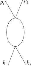
Figure 2: The Feynman diagram equivalent to the second term $\int{d\xi}\left\langle{p_{1}p_{2}\left|{T[S_{1}(\frac{\xi}{2})S_{1}(-\frac{\xi}{2})]}\right|k_{1}k_{2}}\right\rangle$ . Only the s-channel diagram is shown.

One finds,

$$\Gamma_{s}=\frac{{9g^{2}}}{{8\pi^{2}}}\int\limits_{1}^{\infty}{d\tau_{1}\int\limits_{1}^{\infty}{d\tau_{2}}}\frac{{e^{-\frac{{(P)^{2}}}{{\Lambda^{2}}}\frac{{\tau_{1}\tau_{2}}}{{\tau_{1}+\tau_{2}}}}}}{{(\tau_{1}+\tau_{2})^{2}}}$$

where $P^{2}=-(p_{1}+p_{2})^{2}=-s$ and is positive in Euclidean space. We employ [6],

$$\int\limits_{1}^{\infty}{d\tau_{1}\int\limits_{1}^{\infty}{d\tau_{2}}=}\int\limits_{\frac{1}{2}}^{1}{dx\int\limits_{\frac{1}{{1-x}}}^{\infty}{\tau d\tau}}+\int\limits_{0}^{\frac{1}{2}}{dx\int\limits_{\frac{1}{x}}^{\infty}{\tau d\tau}}$$

[where $\tau=\tau_{1}+\tau_{2}$ and $x=\frac{\tau_{2}}{\tau}$] and find

$$\Gamma_{s}=\frac{{9g^{2}}}{{8\pi^{2}}}\left({\int\limits_{\frac{1}{2}}^{1}{dx\int\limits_{\frac{1}{{1-x}}}^{\infty}{d\tau+\int\limits_{0}^{\frac{1}{2}}{dx\int\limits_{\frac{1}{x}}^{\infty}{d\tau}}}}}\right)\frac{{e^{-\frac{P^{2}}{{\Lambda^{2}}}\tau(1-x)x}}}{{\tau}}$$

setting $t=\frac{P^{2}}{{\Lambda^{2}}}\tau(1-x)x$

$$\Gamma_{s} = \frac{{9g^{2}}}{{8\pi^{2}}}\left({\int\limits_{\frac{1}{2}}^{1}{dx\int\limits_{\frac{{P^{2}x}}{{\Lambda^{2}}}}^{\infty}{dt+\int\limits_{0}^{\frac{1}{2}}{dx\int\limits_{\frac{{P^{2}(1-x)}}{{\Lambda^{2}}}}^{\infty}{dt}}}}}\right)\frac{{e^{-t}}}{t}$$

$$= \frac{{9g^{2}}}{{8\pi^{2}}}\int\limits_{\frac{1}{2}}^{1}{dx\Gamma\left(0,\frac{{P^{2}x}}{{\Lambda^{2}}}\right)+\int\limits_{0}^{\frac{1}{2}}{dx\Gamma\left(0,\frac{{P^{2}(1-x)}}{{\Lambda^{2}}}\right)}};$$

$$= \frac{{9g^{2}}}{{4\pi^{2}}}\int\limits_{\frac{1}{2}}^{1}{dx\Gamma(0,\frac{{P^{2}x}}{{\Lambda^{2}}}){\rm{}}}$$

$$= \frac{{9g^{2}}}{{4\pi^{2}}}\int\limits_{\frac{1}{2}}^{1}{dx\left[{-\ln\frac{{P^{2}x}}{{\Lambda^{2}}}-\gamma-\sum\limits_{n=1}^{\infty}{\frac{{(-\frac{{P^{2}x}}{{\Lambda^{2}}})^{n}}}{{n(n!)}}}}\right]}$$

$$= \frac{{9g^{2}}}{{8\pi^{2}}}\left({-\ln\frac{s}{{\Lambda^{2}}}+constant-2\sum\limits_{n=1}^{\infty}{\frac{{1}}{{n(n+1)!}}\left({\frac{s}{{\Lambda^{2}}}}\right)^{n}\left({1-\frac{1}{{2^{n+1}}}}\right)}}\right)$$

where, $\Gamma\left(n,z\right)$ is the incomplete $\Gamma$-function

$$\Gamma(n,z)\equiv\int\limits_{z}^{\infty}{\frac{{dt}}{t}}t^{n}e^{-t}$$

Adding up $s,t,u$-channels together,

$$\Gamma(s,t,u) = \frac{{9g^{2}}}{{8\pi^{2}}}\left[{-\ln\frac{s}{{\Lambda^{2}}}-\ln\frac{t}{{\Lambda^{2}}}-\ln\frac{u}{{\Lambda^{2}}}+constant}\right.$$

$$\left.{-2\sum\limits_{n=1}^{\infty}{\frac{{1}}{{\left(n+1\right)(n!)}}\left({\left({\frac{s}{{\Lambda^{2}}}}\right)^{n}+\left({\frac{t}{{\Lambda^{2}}}}\right)^{n}+\left({\frac{u}{{\Lambda^{2}}}}\right)^{n}}\right)\left({1-\frac{1}{{2^{n+1}}}}\right)}}\right]$$

As we shall be interested in the nontrivial contribution arising from nonlocal effects, we shall find it convenient to filter out the usual local effects. We parametrize the local part of the above expression as

$$l\left(\theta\right)=c_{1}+c_{2}ln\left(1-cos^{2}\theta\right)$$

Using (14),

$$l\left(\theta\right) = c^{\prime}_{1}+c_{2}\left(\frac{5}{3}P_{2}(\cos\theta)+\frac{9}{{10}}P_{4}(\cos\theta)+\frac{{13}}{{21}}P_{6}(\cos\theta)+....\right)$$

So that, the quantity entering in the equation (17) is

$$l\left(\theta\right)-\overline{l}\left(\theta\right)=c_{2}\left(\frac{5}{3}P_{2}(\cos\theta)+\frac{9}{{10}}P_{4}(\cos\theta)+\frac{{13}}{{21}}P_{6}(\cos\theta)+....\right)$$

Now, consider

$$h\left(\theta\right) = \alpha P_{2}\left(cos\theta\right)+\beta P_{4}\left(cos\theta\right)$$

$h\left(\theta\right)$ is the simplest non-trivial even polynomial orthogonal to $l\left(\theta\right)-\overline{l}\left(\theta\right)$ provided

$$\frac{2}{3}\alpha+\frac{1}{5}\beta=0$$

We choose to integrate (17) with $h\left(\theta\right)$. Thus the CV signaling amplitude may be conveniently as

$$\int dcos\theta h\left(\theta\right)\left\{\frac{32\omega^{3}p}{3g^{3}}\left[\frac{{d\sigma}}{{d\Omega}}\right]+(2\pi)^{4}\frac{p\omega_{p}}{2}Im\left\{\int{d\xi}\left\langle{p_{1}p_{2}\left|{T[S_{1}(\frac{\xi}{2})S_{1}(-\frac{\xi}{2})]}\right|k_{1}k_{2}}\right\rangle\right\}\right\}$$

where we have dropped the two terms with angular averages as $\int dcos\theta h\left(\theta\right)\times constant=0$.

6 $O\left(g^{4}\right)$ contributions

We shall calculate $O\left(g^{4}\right)$ terms in $\mathcal{R}$ of equation (15) and find the range of couplings and energies when it is ignorable. Calculations of quantities required for this has already been done in a local theory. As such quantities in a nonlocal theory will differ only by terms of $O\left(\frac{1}{\Lambda^{2}}\right)$ from a local theory and we are interested only in an estimate of such terms in $\mathcal{R}$, we shall employ the local results for this purpose.

6.1 the $S_{1}S_{3}$-type terms

One of the contributions to $\frac{d\sigma}{d\Omega}$ we have not taken account of is the $O\left(g^{4}\right)$ contribution coming from a term of the kind $S_{1}S_{3}$ in $\mathcal{R}$. To evaluate this we need to calculate $O\left(g^{3}\right)$ contribution to S-matrix coming from the two loop diagrams.

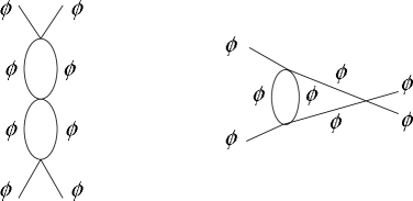
Figure 3: Diagrams contributing to 2 particle matrix element of $S_{3}$. Diagrams obtained by interchanges of momentum labels are not shown.

These two loop diagrams have already been computed in the context of the standard model [16] with the renormalization convention which amounts to using a mass scale $\sim m$. We shall adopt the result to the case of $\phi^{4}$ theory and employ them with our renormalization convention. The leading terms in the amplitude $A\left(s,t,u\right)$ comes from the $ln^{2}s,\,ln^{2}t,\,ln^{2}u$ terms for $s$ large. Keeping these terms, and using the renormalization convention of [16], the full amplitude $A\left(s,t,u\right)$ is [here, $\hat{s}=\frac{s}{m^{2}}$ etc.]

$$A(s,t,u) = -6g+\frac{{g^{2}}}{{16\pi^{2}}}\left[{-18\left({\ln(-\hat{s})+\ln(-\hat{t})+\ln(-\hat{u})}\right)}\right]$$

$$+ \frac{{g^{3}}}{{\left({16\pi^{2}}\right)^{2}}}\left[{-162\left({\ln^{2}(-\hat{s})+\ln^{2}(-\hat{t})+\ln^{2}(-\hat{u})}\right)+.....}\right]$$

$$\equiv -6g+g^{2}a+g^{3}b$$

Where,

$$a = \frac{1}{{16\pi^{2}}}\left[{-18\left({\ln(\frac{{-s}}{{m^{2}}})+\ln(\frac{{-t}}{{m^{2}}})+\ln(\frac{{-u}}{{m^{2}}})}\right)}\right]$$

$$b = \frac{1}{{\left({16\pi^{2}}\right)^{2}}}\left[{-162\left({\ln^{2}(\frac{{-s}}{{m^{2}}})+\ln^{2}(\frac{{-t}}{{m^{2}}})+\ln^{2}(\frac{{-u}}{{m^{2}}})}\right)+.....}\right]$$

We define $\tilde{g}$ by evaluating $Re\left[A\left(s,t,u\right)\right]$ at $s=-2s_{0}+2m^{2},\;t=u=s_{0}+m^{2}$. We have,

$$\begin{array}[]{l}-6\tilde{g}=-6g+g^{2}\tilde{a}+g^{3}\tilde{b}+O(g^{4})\end{array}$$ (18)

Where,

$$\tilde{a} = \frac{1}{{16\pi^{2}}}\left[{-18\left({\ln(\frac{{2s_{0}}}{{m^{2}}})+2\ln(\frac{{s_{0}}}{{m^{2}}})}\right)}\right]$$

$$\tilde{b} = \frac{1}{{\left({16\pi^{2}}\right)^{2}}}\left[{-162\left({\ln^{2}(\frac{{2s_{0}}}{{m^{2}}})+2\ln^{2}(\frac{{s_{0}}}{{m^{2}}})}\right)+.....}\right]$$

Now from (18),

$$-6g = -6\tilde{g}-g^{2}\tilde{a}-g^{3}\tilde{b}+O(g^{4})$$

$$= -6\tilde{g}-\left({\tilde{g}+\frac{{g^{2}}}{6}\tilde{a}+..}\right)^{2}\tilde{a}-\left({\tilde{g}+\frac{{g^{2}}}{6}\tilde{a}+..}\right)^{3}\tilde{b}+O(\tilde{g}^{4})$$

$$= -6\tilde{g}-\tilde{g}^{2}\tilde{a}-\tilde{g}^{3}\left({\frac{{\tilde{a}^{2}}}{3}+\tilde{b}}\right)+O(\tilde{g}^{4})$$

So that we can express $A\left(s,t,u\right)$ in terms of $\tilde{g}$ as,

$$A(s,t,u) = -6g+g^{2}a+g^{3}b$$

$$= -6\tilde{g}-\tilde{g}^{2}\tilde{a}-\tilde{g}^{3}\left({\frac{{\tilde{a}^{2}}}{3}+\tilde{b}}\right)+\tilde{g}^{2}a+\tilde{g}^{3}b+\frac{{\tilde{g}^{3}}}{3}\tilde{a}a+o(\tilde{g}^{4})$$

$$= -6\tilde{g}-\tilde{g}^{2}(\tilde{a}-a)-\tilde{g}^{3}\left({\frac{{\tilde{a}^{2}}}{3}+\tilde{b}-b-\frac{{\tilde{a}a}}{3}}\right)+o(\tilde{g}^{4})$$

where,

$$\tilde{a}-a=\frac{1}{{16\pi^{2}}}\left[{-18\left\{{\ln\left({\frac{{2s_{0}}}{s}}\right)+\ln\left({\frac{{s_{0}}}{t}}\right)+\ln\left({\frac{{s_{0}}}{u}}\right)}\right\}}\right]$$

To calculate the relevant matrix element of $S_{3}$, we need to focus our attention on the coefficient of $\tilde{g}^{3}$

$$\frac{{\tilde{a}^{2}}}{3}+\tilde{b}-b-\frac{{\tilde{a}a}}{3}$$

$$= \frac{1}{{\left({16\pi^{2}}\right)^{2}}}\left\{{108\left[{\left({\ln(\frac{{2s_{0}}}{{m^{2}}})+2\ln(\frac{{s_{0}}}{{m^{2}}})}\right)^{2}}\right.}\right.$$

$$- \left.{\left({\ln(\frac{{2s_{0}}}{{m^{2}}})+2\ln(\frac{{s_{0}}}{{m^{2}}})}\right)\left({\ln(\frac{{-s}}{{m^{2}}})+\ln(\frac{{-t}}{{m^{2}}})+\ln(\frac{{-u}}{{m^{2}}})}\right)}\right]$$

$$- \left.{162\left({\ln^{2}(\frac{{2s_{0}}}{{m^{2}}})+\ln^{2}(\frac{{s_{0}}}{{m^{2}}})+\ln^{2}(\frac{{s_{0}}}{{m^{2}}})-\ln^{2}(\frac{{-s}}{{m^{2}}})-\ln^{2}(\frac{{-t}}{{m^{2}}})-\ln^{2}(\frac{{-u}}{{m^{2}}})}\right)}\right\}$$

$$= \frac{1}{{\left({16\pi^{2}}\right)^{2}}}\left\{{162\left({\ln^{2}(1-\cos\theta)+\ln^{2}(1+\cos\theta)}\right)}\right.$$

$$+ \left.{\left({162\times 2\ln\left({\frac{{2p^{2}}}{{m^{2}}}}\right)-108\ln\left({\frac{{2s_{0}^{3}}}{{m^{6}}}}\right)}\right)\ln(1-\cos^{2}\theta)+(\theta-\textup{independent terms})}\right\}$$

$$= \frac{1}{{\left({16\pi^{2}}\right)^{2}}}\left\{{162\left({\ln^{2}(1-\cos\theta)+\ln^{2}(1+\cos\theta)}\right)}\right.$$

$$+ \left.{\left({\frac{{162\times 2}}{3}\ln\left({\frac{{8p^{6}}}{{m^{6}}}}\right)-108\ln\left({\frac{{2s_{0}^{3}}}{{m^{6}}}}\right)}\right)\ln(1-\cos^{2}\theta)+(\theta-\textup{independent terms})}\right\}$$

$$= \frac{1}{{\left({16\pi^{2}}\right)^{2}}}\left\{{162\left({\ln^{2}(1-\cos\theta)+\ln^{2}(1+\cos\theta)}\right)}\right.$$

$$+ \left.{108\ln\left({\frac{{4p^{6}}}{{s_{0}^{3}}}}\right)\ln(1-\cos^{2}\theta)+(\theta-\textup{independent terms})}\right\}$$

Thus,

$$A(s,t,u) = -6\tilde{g}-\frac{{\tilde{g}^{2}}}{{16\pi^{2}}}\left[{-18\left\{{\ln\left({\frac{{2s_{0}}}{s}}\right)+\ln\left({\frac{{s_{0}}}{t}}\right)+\ln\left({\frac{{s_{0}}}{u}}\right)}\right\}}\right]$$

$$- \frac{{\tilde{g}^{3}}}{{\left({16\pi^{2}}\right)^{2}}}\left\{{162\left({\ln^{2}(1-\cos\theta)+\ln^{2}(1+\cos\theta)}\right)}\right.$$

$$+ \left.{108\ln\left({\frac{{s^{3}}}{{16s_{0}^{3}}}}\right)\ln(1-\cos^{2}\theta)+(\theta-\textup{independent terms})}\right\}+o(\tilde{g}^{4})$$

Suppose, we choose the renormalization scale $s_{0}=0.1\Lambda^{2}$. The angular dependence of the relevant matrix element of $S_{3}$ is determined by

$$g\left(\theta\right) = \left[2\left[\ln(\frac{s}{{}^{{}_{0.2\times\sqrt[3]{2}\Lambda^{2}}}})\right]\ln(1-\cos^{2}\theta)+\ln^{2}(1+\cos\theta)+\ln^{2}(1-\cos\theta)\right]$$

we define,

$$a^{\prime}_{2} = \frac{5}{2}\int\limits_{-1}^{1}{d\cos\theta}P_{2}(\cos\theta)g\left(\theta\right)$$

We find,

$$a^{\prime}_{2} = \frac{5}{2}\times\frac{49}{18}+2\ln(\frac{s}{0.252\Lambda^{2}})\left(\frac{-5}{3}\right)$$

$$= 6.81-3.33ln(15.87\frac{p^{2}}{\Lambda^{2}})$$

putting in some values for $p^{2}/\Lambda^{2}$, we find

$\frac{p^{2}}{\Lambda^{2}}$	0.1	0.2	0.4	0.8
$a^{\prime}_{2}$	5.27	2.96	0.66	-1.65

Table 2: Legendre coefficient $a_{2}^{\prime}$ for some values of $\frac{p^{2}}{\Lambda^{2}}$.

Contribution from $S_{1}S_{3}$ term in terms of Legendre coefficient turns out to be

$$a_{2}^{(4,1)}=\frac{81\tilde{g^{4}}}{64\pi^{4}}a_{2}^{\prime}$$

To compare this particular $O\left(g^{4}\right)$ contribution to the non-local term, we consider,

$$\frac{a_{2}^{\left(4,1\right)}}{a_{2}^{nonlcal}} = \frac{27\widetilde{g^{2}}}{16\pi^{2}}\frac{a^{\prime}_{2}}{\left({\frac{{p^{2}}}{{\Lambda^{2}}}}\right)^{2}}$$

with, $\frac{{6g}}{{16\pi^{2}}}=0.001$(comparable to $\frac{\alpha}{4\pi}$ in electrodynamics), we tabulate the ratio for different values of $\frac{p^{2}}{\Lambda^{2}}=\frac{s}{4\Lambda^{2}}$:

$\frac{p^{2}}{\Lambda^{2}}$	0.1	0.2	0.4	0.8
$\frac{a_{2}^{\left(4,1\right)}}{a_{2}^{nonlcal}}$	0.062	0.0088	0.0005	-0.0003

Table 3: Comparison of $S_{1}S_{3}$-type terms with the leading non-local contribution.

We saw earlier in section 3 that it was possible to discern CV for $\frac{p^{2}}{\Lambda 2}\gtrsim 0.2$. In the same range of momenta, we find that contribution of this $O\left(\widetilde{g}^{4}\right)$ term small enough to be ignored.

6.2 the$\left|{S_{2}}\right|^{2}$ term

The contribution of this term is,

$$= \left({\frac{{9\widetilde{g}^{2}}}{{8\pi^{2}}}\ln\frac{{stu}}{{2s_{0}^{3}}}}\right)^{2}$$

$$= \left({\frac{{9\widetilde{g}^{2}}}{{8\pi^{2}}}}\right)^{2}\left[{\ln\frac{{8p^{6}}}{{s_{0}^{3}}}+\ln(1-\cos^{2}\theta)}\right]^{2}$$

$$= \left({\frac{{9\widetilde{g}^{2}}}{{8\pi^{2}}}}\right)^{2}\left[{\ln^{2}\frac{{s^{3}}}{{8s_{0}^{3}}}+\ln^{2}(1-\cos^{2}\theta)+2\ln\frac{{s^{3}}}{{8s_{0}^{3}}}\ln(1-\cos^{2}\theta)}\right]$$

$$= \left({\frac{{9\widetilde{g}^{2}}}{{8\pi^{2}}}}\right)^{2}\left[{\ln^{2}\left({\frac{{s^{3}}}{{8s_{0}^{3}}}}\right)+\ln^{2}(1-\cos\theta)+\ln^{2}(1+\cos\theta)+2\ln(1-\cos\theta)\ln(1+\cos\theta)+}\right.$$

$$\left.{2\times 3\ln\left({\frac{s}{{2s_{0}}}}\right)\ln(1-\cos^{2}\theta)}\right]$$

The relevant angular dependent part is given below:

$$f(\theta) = \left[{\ln^{2}(1-\cos\theta)+\ln^{2}(1+\cos\theta)+2\ln(1-\cos\theta)\ln(1+\cos\theta)+}\right.$$

$$\left.{2\times 3\ln\left({\frac{s}{{2s_{0}}}}\right)\ln(1-\cos^{2}\theta)}\right]$$

Defining

$$a^{\prime\prime}_{2}=\frac{5}{2}\int\limits_{-1}^{+1}{d\cos\theta P_{2}(\cos\theta)f(\theta)},$$

we obtain,

$$a^{\prime\prime}_{2} = \frac{5}{2}\times\frac{{49}}{{18}}-\frac{{25}}{{18}}+2\left({3\ln\frac{{s}}{{0.2\Lambda^{2}}}}\right)\left({\frac{{-5}}{3}}\right)$$

$$= 5.42-10\left({\ln\frac{20p^{2}}{{\Lambda^{2}}}}\right)$$

We complete the table of $\frac{p^{2}}{{\Lambda^{2}}}$ versus $a^{\prime\prime}_{2}$.

$\frac{p^{2}}{{\Lambda^{2}}}$	$0.1$	$0.2$	$0.4$	$0.8$
$a^{\prime\prime}_{2}$	-1.51	-8.44	-15.4	-22.3

Table 4: Legendre coefficient $a_{2}^{\prime\prime}$ for some values of $\frac{p^{2}}{\Lambda^{2}}$ .

$\left|{S_{2}}\right|^{2}$ term contributes the following Legendre coefficient:

$$a_{2}^{\left(4,2\right)} = \frac{{81\tilde{g}^{4}}}{{64\pi^{4}}}\times a^{\prime\prime}_{2}$$

Now, adding the Legendre coefficients to get the total contribution to $\mathcal{R}$ in $O\left(g^{4}\right)$:

$$a_{2}^{\left(4\right)}=a_{2}^{\left(4,1\right)}+a_{2}^{\left(4,2\right)}=\frac{{81\tilde{g}^{4}}}{{64\pi^{4}}}\left({a^{\prime}_{2}+a^{\prime\prime}_{2}}\right)$$

Comparison of nonlocal effects of $O\left(g^{2}\right)$ and local terms of next order is facilitated by looking at the ratio $r$:

$$r=\frac{{a_{2}^{\left(4\right)}}}{{a_{2}^{nonlocal}}}=\frac{{27\tilde{g}^{2}}}{{16\pi^{2}}}\frac{{\left({a^{\prime}_{2}+a_{2}^{\prime\prime}}\right)}}{{\left({\frac{{p^{2}}}{{\Lambda^{2}}}}\right)^{2}}}$$

We tabulate $r$ for various $\frac{p^{2}}{\Lambda^{2}}$ and with $\frac{{6\tilde{g}}}{{16\pi^{2}}}=10^{-3}$:

$\frac{p^{2}}{\Lambda^{2}}$	0.1	0.2	0.4	0.8
$a_{2}^{\left(4\right)}$	2.34$\times 10^{-8}$	-3.42$\times 10^{-8}$	-9.19$\times 10^{-8}$	-1.49$\times 10^{-7}$
$|r|$	0.04	.02	0.01	0.004

Table 5: Final comparison of neglected terms of $O\left(\widetilde{g}^{4}\right)$ in (17) with the CV amplitude.

Thus, the contribution from the terms of $O\left(g^{4}\right)$ we neglected is indeed a few percent at best in this range of $\frac{p^{2}}{\Lambda^{2}}$ and couplings.

7 conclusions

We argued that physical theories may develop a small causality violation at high enough energies; which could be due to diverse causes such as a fundamental length scale, composite structure of standard model particles etc. We wanted to study how it can be observed experimentally. We considered as a model theory, the nonlocal scalar theory, which embodies quantum violations of causality. We demonstrated that CV could be observed by usual laboratory measurements which obtain $\frac{d\sigma}{d\Omega}$ for the exclusive elastic process $\phi\phi\rightarrow\phi\phi$. Analysis of local contribution versus the non-local CV amplitude enabled one to conclude that CV effects can be noticeable at $s\sim\Lambda^{2}$ where $\Lambda$ is the large mass scale present in the theory and a way to demonstrate its existence is via an analysis of the angular distribution of scattering cross-section. We constructed an observable that would serve the purpose if higher order effects are negligible. We analyzed these $O\left(g^{4}\right)$ terms and demonstrated that they are indeed negligible compared to the CV terms at energies $s\leq\Lambda^{2}$ and for a typical coupling comparable to electromagnetic coupling $\frac{\alpha}{4\pi}$. A work, along the same lines, but applicable to the realistic cases of experimentally observed exclusive processes $e^{+}e^{-}\rightarrow e^{+}e^{-}$, $e^{+}e^{-}\rightarrow\mu^{+}\mu^{-}$ and $e^{+}e^{-}\rightarrow\tau^{+}\tau^{-}$ is in progress.

ACKNOWLEDGEMENT
AH would like to thank NISER, Bhubaneswar for support where a part of the work was done.

References

- [1] A. Pais and G. E. Uhlenbeck, Phys. Rev. 79, 145-165 (1950).
- [2] S. D. Joglekar, hepth/0601006
- [3] See, e.g. K. Namsrai, Nonlocal Quantum Field Theory and Stochastic Quantum Mechanics (D. Reidel Publishing company).
- [4] J.Moffat Phys. Rev. D41,1177(1990)
- [5] See e.g. N. Seiberg, Leonard Susskind, N. Toumbas; JHEP 0006:044,(2000)
- [6] G. Kleppe and R. P. Woodard, Nucl. Phys. B388, 81 (1992)
- [7] D. A. Eliezer, and R. P. Woodard, Nucl.Phys.B 325, 389 (1989).
- [8] E. D. Evens et al, Phys Rev D43, 499 (1991)
- [9] S.D.Joglekar, J. Phys. A34, 2765-2776 (2001)
- [10] S.D.Joglekar,Int.J.Mod. Phys.A 16, (2001).
- [11] S. D. Joglekar and G. Saini, Z. Phys. C.76, 343-353 (1997); A. Basu, and S. D. Joglekar, J. Math. Phys. 41, 7206-7219 (2000).
- [12] N. J. Cornish, Int.J.Mod. Phys.A 7, 6121-6157 (1992).
- [13] A. Jain and S.D.Joglekar, Int.J. Mod. Phys.A 19, 3409(2004)
- [14] S.D. Joglekar, Int. J. of Theo. Phys.47, (2008)
- [15] N.N.Bogolibov and D.V.Shirkov, ‘Introduction to Theory of Quantized Fields’ ( ed.), John Wiley(1980). See pg. 200-220.
- [16] P.N. Maher, L. Durand, K. Reiselmann Phys.Rev. D 48,1061(1993)
- [17] M. E. Peskin, and D. V. Schroeder, An introduction to quantum field theory (Westview, Boulder, Colo., 2003)
- [18] A. Ayyer and S.D.Joglekar (Unpublished work)