Infrared regularization with vector mesons and baryons

Abstract:

We extend the method of infrared regularization to spin-1 fields coupled to baryons. As an application, we discuss the axial form factor of the nucleon.

1 Introduction

In a recent work [1], the scheme of infrared regularization (developed in its original form by Becher and Leutwyler [2]) was extended to the case of explicit meson resonances interacting with soft pions, as e.g. the first step towards a systematic inclusion of vector mesons in the meson sector of Chiral Perturbation Theory (ChPT). It is the aim of this article to provide a further extension of infrared regularization to the situation where baryons as well as vector mesons are present. This can be considered as a synthesis of the results in [1] and [2]. Such an extension is not only of interest in itself, but can be applied to a plethora of observables, where vector and axial-vector mesons are known to play an important role, such as the electroweak form factors of the nucleon. As one example we mention the contribution of the $\pi\rho$ loop to the strangeness form factors of the nucleon [3, 4].

Infrared regularization (IR) is a solution to the following problem. The presence of mass scales which must be considered as ’heavy’ compared to the masses and momenta of the soft pions will in general mess up the usual power counting rules of ChPT by which the perturbation series of the effective theory is ordered [5, 6, 7]. This observation was first made when baryons were incorporated in the framework of ChPT [8] (for a recent review on baryon ChPT we refer to [9]). The procedure of infrared regularization separates the (dimensionally regularized) one-loop graphs of baryon ChPT into a part which stems from the soft pion contribution and a part generated from loop momenta close to the ’heavy’ scale. The latter portion of the loop graph, called the ’regular’ part, will usually not be in accord with the low-energy power counting, but can always be absorbed in local terms derived from the effective Lagrangian. It is therefore dropped from the loop graph, and only the first part, called the infrared singular part of the loop integral, is kept. Though both the vector mesons and the baryons interact as ’heavy’ particles with the pions, the power counting is different for the two species, at least for the kinds of Feynman graphs we consider in this work. There, the vector mesons appear only as internal lines with small momenta far from their mass shell, so that the resonance propagator is counted as $O(q^{0})$ (where $q$ indicates some small momentum scale or Goldstone boson mass), while the baryon propagator is counted as $O(q^{-1})$, since the baryon is pushed from its mass shell only by a small amount due to its interaction with the soft pions and vector mesons. In the graphs we treat here, only one single baryon is present, with the baryon line running through the diagram undergoing only soft interactions. The number of the virtual vector mesons, however, is not fixed. The pion propagator is counted as $O(q^{-2})$, as usual, both the pion momentum and the pion mass being of $O(q)$. Appropriate powers of $q$ are also assigned to vertices from the effective Lagrangian. Finally, the measure of every $d$-dimensional loop integration is booked as $O(q^{d})$. This counting scheme applies, of course, to tree graphs, but also to the infrared singular, or soft, parts of the loop graphs. The regular parts of the loop graphs are not guaranteed to obey the power counting rules. These general remarks will be exemplified in the following sections.

Before working out the case where both baryons and vector mesons appear in a Feynman diagram, we will briefly review the scheme of infrared regularization for loop integrals where only one heavy scale shows up. This will not only serve to give a unified presentation of the method, but also provide some results needed for an application of the general scheme to the axial form factor of the nucleon. Before starting with the presentation of the formalism, let us mention that the loop integrals studied in this work have also been treated, using a different regularization scheme which is in some respect complementary to the one used here, in Ref. [10].

2 IR regularization in the pion-nucleon system

When only pions and nucleons are treated as explicit fields of the effective theory, the fundamental loop integral one has to consider is

$$I_{MB}(p^{2})=\int\frac{d^{d}l}{(2\pi)^{d}}\frac{i}{((p-l)^{2}-m^{2})(l^{2}-M^{2})}.$$ (1)

Here, $M$ is the pion mass (being of chiral order $O(q)$) and $m$ is the nucleon mass. Applying the low-energy power counting scheme outlined in the introduction, one would assign a chiral order of $q^{d-3}$ to this integral. We will see in a moment that only an appropriately extracted low-energy part of $I_{MB}$ will obey this power counting requirement.

All the other pion-nucleon loop integrals are either only trivially modified by the infrared regularization scheme, or they can be derived from eq. (1) (see sec. 6 of [2]). For example, the scalar tadpole integral containing only the pion propagator is not modified at all, as there is no ’hard momentum’ structure present that could lead to a nonvanishing regular part of this integral. Thus we have

$$I_{M}^{IR}=I_{M}=\int\frac{d^{d}l}{(2\pi)^{d}}\frac{i}{l^{2}-M^{2}},$$

and a direct calculation gives

$$I_{M}^{IR}=\frac{\Gamma(1-\frac{d}{2})}{(4\pi)^{\frac{d}{2}}}M^{d-2}.$$ (2)

Note the typical structure of the $d$-dependent power of the pion mass. For arbitrary values of the dimension parameter $d$, $I_{M}^{IR}$ is in general proportional to fractional powers of $M^{2}$, and will even diverge in the so-called chiral limit where the quark masses $m_{u},m_{d}$ go to zero (so that also $M\rightarrow 0$) for small enough $d$ (we mostly consider the two–flavor case here but the method can be trivially extended to include also strange quarks). Such terms will never occur in the regular parts of the loop integrals which stem from the high-momentum region of the integration: those parts are always expandable in the pion mass. The baryon tadpole integral, e.g., is

$$I_{B}=\int\frac{d^{d}l}{(2\pi)^{d}}\frac{i}{l^{2}-m^{2}},$$

and is trivially expandable in $M^{2}$, since it has no pion mass dependence at all. Therefore one has $I_{B}^{IR}=0$. These remarks may serve to explain the terminology ’infrared singular’ vs. ’regular’.

Returning to eq. (1), we must extract the part of this integral that is proportional to some $d$-dependent power of $M$, like in eq. (2). One can think of this extraction prescription as an operational definition of infrared regularization. The method is explained in full generality in [2]. Here, we concentrate on the case with on-shell momentum $p$, i.e. $p^{2}=m^{2}$. This shows all the features we need for the demonstration, and also yields the result we will use in our application of the scheme in sec. 4. We introduce a Feynman parameter integration in the usual way:

$$I_{MB}=\int\frac{d^{d}l}{(2\pi)^{d}}\int_{0}^{1}\frac{dz}{[((p-l)^{2}-m^{2})z+(l^{2}-M^{2})(1-z)]^{2}}.$$ (3)

Performing the standard steps, we find for $p^{2}=m^{2}$:

$$I_{MB}=-m^{d-4}\frac{\Gamma(2-\frac{d}{2})}{(4\pi)^{\frac{d}{2}}}\int_{0}^{1}\frac{dz}{(z^{2}-\alpha z+\alpha)^{2-\frac{d}{2}}},$$ (4)

where we have defined $\alpha=M^{2}/m^{2}$ (note the difference to ref.[2], where this letter is reserved for $\alpha_{\mathrm{BL}}=M/m$). Fractional powers of the small variable $\alpha$ will be produced near $z=0$: there, the integrand is approximately $(\alpha)^{\frac{d}{2}-2}$. For small enough $d$, there would be an infrared singularity for $M\rightarrow 0$ located in parameter space at $z=0$. It can already be seen from eq. (3) that the parameter region near $z=0$ is associated with the low-energy portion of the integral: In this region, only the ’soft’ pion propagator is weighted in the loop integration, while the hard momentum structure of the nucleon propagator dominates near $z=1$. The extraction of the part of the integral proportional to $d$-dependent powers of $\alpha$ now proceeds as follows: the parameter integration is split into two parts like

$$\int_{0}^{1}=\int_{0}^{\infty}-\int_{1}^{\infty}.$$ (5)

We will first show that the second integral on the r.h.s. is regular, i.e. expandable, in the variable $\alpha$. This is easy to see, because for $z\geq 1$, the integrand can be expanded like

$$(z^{2}-\alpha z+\alpha)^{\frac{d}{2}-2}=z^{d-4}\sum_{k=0}^{\infty}\frac{\Gamma(2-\frac{d}{2}+k)}{\Gamma(2-\frac{d}{2})}\frac{\alpha^{k}}{k!}\biggl{(}\frac{z-1}{z^{2}}\biggr{)}^{k}.$$ (6)

Interchanging integration and summation (which is a valid operation at least for some range of $d$), one gets for the regular part

$$R\equiv m^{d-4}\frac{\Gamma(2-\frac{d}{2})}{(4\pi)^{\frac{d}{2}}}\int_{1}^{\infty}\frac{dz}{(z^{2}-\alpha z+\alpha)^{2-\frac{d}{2}}}=m^{d-4}\frac{\Gamma(2-\frac{d}{2})}{(3-d)(4\pi)^{\frac{d}{2}}}+O(\alpha).$$ (7)

At this point we should make the remark that the extension of the parameter integration to infinity will lead to divergences as $d$ increases. The infrared singular or regular parts are then defined as follows: The parameter integrals are computed for the range of $d$ where they are well-defined, and the result will be continued analytically to arbitrary values of $d$. This amounts to the suppression of power divergences of the parameter integrals, which have nothing to do with the infrared singularity at $z=0$, and will be cancelled anyway on the r.h.s. of eq. (5).

Next we must show that the first term on the r.h.s. of eq. (5) is proportional to a $d$-dependent power of $\alpha$. To see this, we substitute $z=\sqrt{\alpha}y$ to get

$$\int_{0}^{\infty}\frac{dz}{(z^{2}-\alpha z+\alpha)^{2-\frac{d}{2}}}=\sqrt{\alpha}^{d-3}\int_{0}^{\infty}\frac{dy}{(y^{2}-\sqrt{\alpha}y+1)^{2-\frac{d}{2}}}.$$

The remaining integral on the r.h.s. will not produce $d$-dependent powers of $\alpha$, since the integrand can be expanded in $\sqrt{\alpha}$ similar to eq. (6). Thus we have found that the parameter integral from zero to infinity is proportional to a $d$-dependent power of $\alpha$. The infrared singular part $I_{MB}^{IR}$ of the loop integral therefore equals

$$I_{MB}^{IR} = -m^{d-4}\frac{\Gamma(2-\frac{d}{2})}{(4\pi)^{\frac{d}{2}}}\int_{0}^{\infty}\frac{dz}{(z^{2}-\alpha z+\alpha)^{2-\frac{d}{2}}}$$ (8)

$$= -\frac{m^{d-4}\sqrt{\alpha}^{d-3}}{2(4\pi)^{\frac{d}{2}}}\sum_{k=0}^{\infty}\frac{\sqrt{\alpha}^{k}}{k!}\Gamma\biggl{(}\frac{k+1}{2}\biggr{)}\Gamma\biggl{(}\frac{3+k-d}{2}\biggr{)}.$$

As $d\rightarrow 4$, this has the well-known leading term

$$I_{MB}^{IR}(d\rightarrow 4)=\frac{1}{16\pi}\biggl{(}\frac{M}{m}\biggr{)}+\ldots,$$

where the dots indicate terms of higher order in $M/m$. This is clearly in accord with the low-energy power counting. In contrast to that, the first term of the expansion of the regular part $R$ obviously violates this counting when $d\rightarrow 4$. The infrared regularization now prescribes to drop $R$ from the loop contribution and substitute $I_{MB}^{IR}$ for $I_{MB}$. Moreover, the poles of $I_{MB}^{IR}$ in $d-4$ are also absorbed in a renormalization of the masses and coupling constants of the effective Lagrangian. Again, for a more general and comprehensive treatment of the IR scheme in the pion-nucleon system, the reader should consult the original article of Becher and Leutwyler [2].

3 IR regularization for vector mesons and pions

In this section, we consider another case of infrared regularization, first examined in [1]. The internal baryon lines from the preceding section are now replaced by vector meson lines, however, the vector mesons do not show up as external particles in the graphs we consider here (an example for the treatment of such a graph can be found in sec. 11 of [1]). The only external particles here are pions (or, in some cases, soft photons etc.), so that there are only small external momenta of order $O(q)$ flowing into the loop. The fundamental scalar loop integral is in this case

$$I_{MV}(q^{2})=\int\frac{d^{d}l}{(2\pi)^{d}}\frac{i}{((q-l)^{2}-M_{V}^{2})(l^{2}-M^{2})},$$ (9)

where $M_{V}$ is the mass of the heavy meson resonance and $q$ is some small external momentum (small with respect to the resonance mass $M_{V}$). This is, in principle, the same function as in eq. (1), so the reader might ask why we devote this section to the examination of this case. The point is that the extraction of the infrared singular part of $I_{MV}$ must proceed along different lines here. As shown in [1], a splitting like that of eq. (5) does not amount to a separation into infrared singular and regular parts as in the preceding section. This can be traced back to the fact that the extension of the parameter integrals to infinity leads to a singular behaviour of the loop function near $q^{2}=0$. Of course, also $I_{MB}^{IR}$ has such a singularity as the external momentum squared goes to zero (see sec. 5.4 of [2]), but the point $p^{2}=0$ lies far outside the low-energy region in that case. Here, however, the point $q^{2}=0$ lies at the center of the low-energy region, so the infrared singular and regular parts can not be expressed as parameter integrals from zero or one to infinity, respectively. For example, a ’regular’ part defined as being proportional to the parameter integral from one to infinity would not be expandable around $q^{2}=0$, as it should be in order to be able to absorb the corresponding terms in a renormalization of the local operators in the effective Lagrangian.

To circumvent this difficulty, we will take up the following simple idea from [1]. We observe that $I_{MV}$ is analytic at $q^{2}=0$, the only singularity being the threshold branch point at $q^{2}=(M_{V}+M)^{2}$, which is far outside the range of small $q^{2}$-values. Expanding $I_{MV}$ in $q^{2}$, the analyticity properties in that variable are obvious. Each coefficient in this expansion can be split into an infrared singular and a regular part almost like in eq. (5). Extracting the infrared singular part proportional to $d$-dependent powers of the pion mass of each coefficient, and resumming the series, one arrives at a well-defined expression for the infrared singular part of the loop integral $I_{MV}$ that is (by construction) expandable in the small variable $q^{2}/M_{V}^{2}$.

To start with the analysis, let us first consider the special case where the external momentum vanishes: $q=0$. Then we have

$$I_{MV}(0) = \int\frac{d^{d}l}{(2\pi)^{d}}\frac{i}{(l^{2}-M_{V}^{2})(l^{2}-M^{2})}$$

$$= \frac{1}{M^{2}-M_{V}^{2}}\biggl{(}\int\frac{d^{d}l}{(2\pi)^{d}}\frac{i}{l^{2}-M^{2}}-\int\frac{d^{d}l}{(2\pi)^{d}}\frac{i}{l^{2}-M_{V}^{2}}\biggr{)}.$$

In the last step of this equation, we have already achieved the splitting into an infrared singular and a regular part, which is quite trivial here. The first term is proportional to a $d$-dependent power of $M$ (compare eq. (2)), while the second part is clearly expandable in $M^{2}$ (because $M_{V}^{2}\gg M^{2}$). Moreover, the pion mass expansion of the first term starts with $M^{d-2}$, in agreement with the low-energy power counting for $I_{MV}$: In contrast to the baryon propagator in sec. 2, the resonance propagator is counted as $O(q^{0})$ since, in the low-energy region, the off-shell momentum of the internal resonance line is far below its mass shell. The counting for the pion propagator and the loop measure is the same as before, and one is lead to the power counting result $q^{d-2}$ for $I_{MV}$. Therefore we can write

$$I_{MV}^{IR}(0)=\frac{1}{M^{2}-M_{V}^{2}}\int\frac{d^{d}l}{(2\pi)^{d}}\frac{i}{l^{2}-M^{2}}.$$ (10)

It should be clear that there will only be corrections of $O(q^{2})$ to this result when we compute the regularized integral for nonvanishing $q$. We introduce the following variables,

$$\tilde{\alpha}=\frac{M^{2}}{M_{V}^{2}}\qquad,\qquad\tilde{\beta}=\frac{q^{2}}{M_{V}^{2}},$$ (11)

which we assume to be small in the sense that $\tilde{\alpha},\tilde{\beta}\ll 1$. Just like in sec. 2, we use the Feynman parameter trick to write

$$I_{MV}(q^{2})=-M_{V}^{d-4}\frac{\Gamma(2-\frac{d}{2})}{(4\pi)^{\frac{d}{2}}}\int_{0}^{1}\frac{dz}{(\tilde{\beta}z^{2}+z(1-\tilde{\alpha}-\tilde{\beta})+\tilde{\alpha})^{2-\frac{d}{2}}}.$$ (12)

We rewrite this expression as follows:

$$I_{MV}(q^{2})=-M_{V}^{d-4}\frac{\Gamma(2-\frac{d}{2})}{(4\pi)^{\frac{d}{2}}}\int_{0}^{1}\frac{dz}{(z(1-\tilde{\alpha}-\tilde{\beta})+\tilde{\alpha})^{2-\frac{d}{2}}}\biggl{(}1+\frac{\tilde{\beta}z^{2}}{z(1-\tilde{\alpha}-\tilde{\beta})+\tilde{\alpha}}\biggr{)}^{\frac{d}{2}-2}.$$

This can be expanded according to

$$I_{MV}(q^{2})=-\frac{M_{V}^{d-4}}{(4\pi)^{\frac{d}{2}}}\sum_{k=0}^{\infty}\frac{\Gamma(\frac{d}{2}-1)}{k!\Gamma(\frac{d}{2}-1-k)}\int_{0}^{1}\frac{\Gamma(2-\frac{d}{2})dz}{(z(1-\tilde{\alpha}-\tilde{\beta})+\tilde{\alpha})^{2-\frac{d}{2}}}\biggl{(}\frac{\tilde{\beta}z^{2}}{z(1-\tilde{\alpha}-\tilde{\beta})+\tilde{\alpha}}\biggr{)}^{k}.$$

In the next step, we extract the infrared singular part of each term in the sum. In each parameter integral, we substitute $z=\tilde{\alpha}y$ and extend the integration range to infinity:

$$I_{k}\equiv\int_{0}^{1}dz\frac{z^{2k}}{(z(1-\tilde{\alpha}-\tilde{\beta})+\tilde{\alpha})^{2+k-\frac{d}{2}}}\rightarrow\int_{0}^{\infty}dy\frac{\tilde{\alpha}^{\frac{d}{2}-1+k}y^{2k}}{(1+y(1-\tilde{\alpha}-\tilde{\beta}))^{2+k-\frac{d}{2}}}.$$ (13)

Divergences of the parameter integral due to the extension of the upper limit to infinity are again handled by analytic continuation in $d$. It can be expressed in terms of Gamma functions:

$$\int_{0}^{\infty}dy\frac{y^{2k}}{(1+y(1-\tilde{\alpha}-\tilde{\beta}))^{2+k-\frac{d}{2}}}=\frac{\Gamma(2k+1)\Gamma(1-\frac{d}{2}-k)}{(1-\tilde{\alpha}-\tilde{\beta})^{2k+1}\Gamma(2-\frac{d}{2}+k)}.$$

This is clearly expandable in the small variables $\tilde{\alpha}$ and $\tilde{\beta}$, so that the r.h.s. of eq. (13) in fact has the proper form of an infrared singular contribution, being proportional to $d$-dependent powers of $\tilde{\alpha}$. Moreover, it is not difficult to see that the parameter integrals from $1$ to infinity are completely regular in the small variables. So, putting pieces together, and using the following identity for Gamma functions:

$$\frac{\Gamma(\frac{d}{2}-1)}{\Gamma(\frac{d}{2}-1-k)}=(-1)^{k}\frac{\Gamma(2-\frac{d}{2}+k)}{\Gamma(2-\frac{d}{2})},\qquad k\in\mathbf{N},$$ (14)

we can sum the series of infrared singular terms and write

$$I_{MV}^{IR}(q^{2})=-\frac{M_{V}^{d-4}}{(4\pi)^{\frac{d}{2}}}(\tilde{\alpha})^{\frac{d}{2}-1}\sum_{k=0}^{\infty}\frac{(-\tilde{\alpha}\tilde{\beta})^{k}}{(1-\tilde{\alpha}-\tilde{\beta})^{2k+1}}\frac{\Gamma(2k+1)\Gamma(1-\frac{d}{2}-k)}{\Gamma(k+1)}.$$ (15)

Note that the leading term in this result is of chiral order $O(q^{d-2})$, as predicted by the power counting scheme. All the terms we have separated off from $I_{MV}$ are regular in both small parameters, and only the infrared singular terms remain. For $\tilde{\beta}=0$, the result for $I_{MV}^{IR}(0)$, which was already established in eq. (10), is reproduced.

It is perhaps worth noting that the result of eq. (15) can be obtained in a different way, which goes back to Ellis and Tang [11, 12]. Though they use their method in the pion-nucleon sector, a variant of it is also applicable here. Their prescription to obtain the soft momentum contribution of a loop integral is the following: Expand the propagators of the heavy particles as if the loop momentum were small, and then interchange summation and loop integration. It is claimed that this prescription eliminates the ’hard momentum’ contributions present in the full loop graph. If this is true, and the concept of hard vs. soft momentum effects is a well-defined one, the result of the procedure should reproduce the infrared singular part of the loop integral in question. Let us see how this works out for our example. Following the prescription just described step by step, we make the following set of transformations:

$$I_{MV}(q^{2}) \rightarrow \int\frac{d^{d}l}{(2\pi)^{d}}\frac{i}{l^{2}-M^{2}}\sum_{k=0}^{\infty}\frac{(2q\cdot l)^{k}}{(q^{2}+l^{2}-M_{V}^{2})^{k+1}}$$

$$\rightarrow \int\frac{d^{d}l}{(2\pi)^{d}}\frac{i}{l^{2}-M^{2}}\sum_{k=0}^{\infty}\frac{(2q\cdot l)^{k}}{(q^{2}+M^{2}-M_{V}^{2})^{k+1}}$$

$$\rightarrow \sum_{k=0}^{\infty}\int\frac{d^{d}l}{(2\pi)^{d}}\frac{i(2q\cdot l)^{k}}{(l^{2}-M^{2})(q^{2}+M^{2}-M_{V}^{2})^{k+1}}.$$

While the first step is just the expansion of the vector meson propagator pole imposed by the prescription, the second step deserves a comment: There, we have used the same trick of partial fractions to split off some hard momentum contributions as in the treatment of $I_{MV}(0)$, but now this was performed $k+1$ times. In the last step, summation and integration were interchanged. Using the formula

$$\int\frac{d^{d}l}{(2\pi)^{d}}\frac{i(q\cdot l)^{2n}}{l^{2}-M^{2}}=(-q^{2}M^{2})^{n}M^{d-2}\frac{\Gamma(n+\frac{1}{2})}{\Gamma(\frac{1}{2})}\frac{\Gamma(1-\frac{d}{2}-n)}{(4\pi)^{\frac{d}{2}}}$$ (16)

and the fact that the loop integrals in the series vanish if $k$ is odd, the result of the transformation is

$$I_{MV}^{\mathrm{soft}}(q^{2})=\frac{M^{d-2}}{(4\pi)^{\frac{d}{2}}}\sum_{n=0}^{\infty}\frac{(-4q^{2}M^{2})^{n}}{(q^{2}+M^{2}-M_{V}^{2})^{2n+1}}\frac{\Gamma(n+\frac{1}{2})\Gamma(1-\frac{d}{2}-n)}{\Gamma(\frac{1}{2})}.$$ (17)

Extracting a factor of $M_{V}^{d-4}$, and using the identity

$$\frac{\Gamma(2n+1)}{\Gamma(n+1)}=4^{n}\frac{\Gamma(n+\frac{1}{2})}{\Gamma(\frac{1}{2})},$$ (18)

we see by comparing to eq. (15) that $I_{MV}^{\mathrm{soft}}=I_{MV}^{IR}$.

In [1], the result for $I_{MV}^{IR}$ was given in a different form (see eqs. (7.10) and (8.4) of that reference). Of course, it is equivalent to the result derived above: it is shown in app. A that the two different forms just amount to a reordering of the corresponding expansions. We will find that the form of eq. (15) is most practical for our purposes, in particular, the chiral expansion can almost immediately be read off from that formula.

In closing this section, we note that the spin or the parity of the resonance obviously do not play a major role in the above considerations. Though we will concentrate on the case of vector mesons, most of what we have said would also apply for other meson resonances, like e.g. scalar or axial-vector mesons.

4 Pion-nucleon system with explicit meson resonances

Now that we have collected the results for the fundamental one-loop integrals in the pion-nucleon and the vector meson-pion sector, we are prepared to extend the framework of infrared regularization once more, and apply it to Feynman graphs where nucleons, pions as well as vector mesons take part in the same loop. The simplest example where this situation occurs is the triangle graph consisting of one pion, one nucleon and one vector meson line. Due to baryon number conservation, the nucleon line must run through the complete diagram. We shall assume that only a small momentum $k$ (small in the usual sense) is transferred at the vector meson-pion vertex. Such a graph will typically contribute to some nucleon form factor in the region of small momentum transfer. With this application in mind, and with the excuse that it will simplify the presentation a bit, we will further specify to on-shell nucleons. Let $p$ and $\bar{p}$ be the four-momenta of the incoming and the outgoing nucleon. Then we have

$$p^{2}=m^{2}=\bar{p}^{2}=(p+k)^{2}\Rightarrow k^{2}=2\bar{p}\cdot k=-2p\cdot k.$$ (19)

Using these kinematic relations, we can rewrite the fundamental scalar loop integral

$$I_{MBV}(k^{2})\equiv\int\frac{d^{d}l}{(2\pi)^{d}}\frac{i}{((p-l)^{2}-m^{2})((k+l)^{2}-M_{V}^{2})(l^{2}-M^{2})}$$ (20)

with the help of the usual Feynman parameter trick, as

$$\int\frac{d^{d}l}{(2\pi)^{d}}\int_{0}^{1}\int_{0}^{1-y}\frac{2idxdy}{(y((p-l)^{2}-m^{2})+x((k+l)^{2}-M_{V}^{2})+(1-x-y)(l^{2}-M^{2}))^{3}}.$$ (21)

Doing the loop integration in the usual manner, we get

$$I_{MBV}(k^{2})=m^{d-6}\frac{\Gamma(3-\frac{d}{2})}{(4\pi)^{\frac{d}{2}}}\int_{0}^{1}\int_{0}^{1-y}\frac{dxdy}{(y^{2}-\alpha y+\alpha+\beta(x^{2}+xy)+x(\gamma-\alpha-\beta))^{3-\frac{d}{2}}},$$ (22)

where the definitions

$$\alpha=\frac{M^{2}}{m^{2}}\ll 1,\qquad\beta=\frac{k^{2}}{m^{2}}\ll 1,\qquad\gamma=\frac{M_{V}^{2}}{m^{2}}\sim O(1).$$

were used. In particular, we have assumed here that the nucleon and the meson resonance are roughly of the same order of magnitude (in the real world, we have $\gamma\sim 2/3$ for the rho resonance, which is good enough for our purposes).
We should remark here that there is, of course, a second graph with the same topology, where the pion and the resonance line are interchanged (see fig. 2). The expression for the corresponding scalar loop integral is

$$\tilde{I}_{MBV}(k^{2})\equiv\int\frac{d^{d}l}{(2\pi)^{d}}\frac{i}{((\bar{p}-l)^{2}-m^{2})((l-k)^{2}-M_{V}^{2})(l^{2}-M^{2})}.$$ (23)

However, the reader can convince himself that, due to the on-shell kinematics specified in eq. (19), this will give exactly the same expression as in eq. (22). Thus, we can focus on the integral $I_{MBV}$.

In analogy to sec. 3, it will be instructive to begin with the special case where $k=0$. Since we must split off the terms where only propagators of heavy particles occur, we can obviously apply the same partial fraction method that led to eq. (10). The remaining pion-nucleon integral can be dealt with as in sec. 2. This gives

$$I_{MBV}^{IR}(0)=\frac{I_{MB}^{IR}(m^{2})}{M^{2}-M_{V}^{2}}.$$ (24)

Having the standard method described of sec. 2 in mind, we note that this equals

$$I_{MBV}^{IR}(0) = m^{d-6}\frac{\Gamma(3-\frac{d}{2})}{(4\pi)^{\frac{d}{2}}}\int_{0}^{\infty}\int_{0}^{\infty}\frac{dxdy}{(y^{2}-\alpha y+\alpha+x(\gamma-\alpha))^{3-\frac{d}{2}}}$$

$$= \frac{m^{d-6}}{(\gamma-\alpha)}\frac{\Gamma(2-\frac{d}{2})}{(4\pi)^{\frac{d}{2}}}\int_{0}^{\infty}\frac{dy}{(y^{2}-\alpha y+\alpha)^{2-\frac{d}{2}}}$$

(compare the last line with the l.h.s of eq. (8)). Once again, the possible divergence for large $d$ at $x\rightarrow\infty$ was regularized by analytic continuation from small $d$ as before. It is reassuring to see that eq. (24) is reproduced in this way.

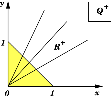
Figure 1: Illustration of the integration ranges for the infrared singular and the regular part of $I_{MBV}$. The shaded triangle is the region integrated over in eq. (22). The three rays indicate the extension of the connections from the soft point at $(0,0)$ to the hard line from $(0,1)$ to $(1,0)$.

The extension of both parameter integrations to infinity is the natural generalization of the prescription used in sec. 2. This can be seen as follows. In eq. (21), we chose our Feynman parameters such that the pion propagator contributes with the weight one at $x=y=0$, while the vector meson and the nucleon propagator have their maximum weight at $(x,y)=(1,0)$ and $(0,1)$, respectively. Consequently, the infrared singularity is located in parameter space at the point $(x,y)=(0,0)$. Indeed, a look at eq. (22) confirms that the integrand in that expression is approximately $\alpha^{\frac{d}{2}-3}$ in the region where $x\sim y\sim 0$, thus producing infrared singular terms there. Far from this region, the integrand is expandable in $\alpha$, as we will show later. To be more specific, imagine the positive quarter of the parameter plane, i.e. $Q_{+}\equiv\{(x,y):x\geq 0,y\geq 0\}$, split in two parts, the first being the triangle one integrates over in the full loop integral (see eq. (22)) and the second part its complement in $Q_{+}$, named $R_{+}$ (see fig. 1 for an illustration). In the latter parameter region, no infrared singularities are located, hence, the integration over this region should yield a proper regular part (there is a qualification here, see below). Geometrically, one might imagine that all lines from the ’soft point’ $(0,0)$ (the location of the infrared singularity in parameter space) to the ’hard line’ from $(0,1)$ to $(1,0)$ are extended to infinity to get the infrared singular part of the loop integral. In a more general setting, there may be soft or hard points, lines, surfaces etc., depending on the number of soft and hard pole structures in the integral under consideration. Extending all connecting lines from the soft point, line etc. to the hard point (line$\ldots$) to infinity, one always achieves a splitting in the original parameter region and a region where no infrared singularities in parameter space are present, analogous to $R_{+}$. It is possible to show that this geometric picture leads to the same results as the prescription given in sec. 6 of [2]. This picture might serve as a guide when trying to split arbitrary one-loop graphs into infrared singular and regular parts, however, one should always convince oneself that both those parts have the correct properties, and that their sum equals the original integral. One has to be a bit careful here, as the following qualification shows. As explained in sec. 3, extending the integration range to infinity might lead to unphysical singularities in variables in which the original integral is analytic (at least in the low-energy region). Those singularities will be harmless if they are located far from the low-energy region, as e.g. the singularity at $s=0$ of the infrared singular parts in the pion-nucleon sector, but in other cases, they can be disturbing. Following the method of [1], we avoided this problem in sec. 3 by expanding the original loop integral in the small variable $\tilde{\beta}$ beforehand. Only then could the integration range be extended to infinity, in each coefficient of the expansion. We must expect that a similar phenomenon will occur in the present case.

To exclude this from the start, we expand $I_{MBV}$ in analogy to eq. (15):

$$I_{MBV}(k^{2}) = \frac{m^{d-6}}{(4\pi)^{\frac{d}{2}}}\sum_{j=0}^{\infty}\frac{\Gamma(\frac{d}{2}-2)}{\Gamma(\frac{d}{2}-2-j)}\int_{0}^{1}\int_{0}^{1-y}\frac{\Gamma(3-\frac{d}{2})dxdy(\beta x(x+y))^{j}}{j!(y^{2}-\alpha y+\alpha+x(\gamma-\alpha-\beta))^{3-\frac{d}{2}+j}}$$

$$= \frac{m^{d-6}}{(4\pi)^{\frac{d}{2}}}\sum_{j=0}^{\infty}\frac{\Gamma(\frac{d}{2}-2)}{\Gamma(\frac{d}{2}-2-j)}\int_{0}^{1}\int_{0}^{1-y}\frac{\Gamma(3-\frac{d}{2})dxdy(\sum_{l=0}^{j}{j\choose l}\beta^{j}x^{l+j}y^{j-l})}{j!(y^{2}-\alpha y+\alpha+x(\gamma-\alpha-\beta))^{3-\frac{d}{2}+j}}.$$

There is still some $\beta$-dependence in the denominator, but in that combination, it will turn out to be harmless. We extend the parameter integrations to $Q_{+}$ and define

$$I_{MBV}^{IR}(k^{2})=\frac{m^{d-6}}{(4\pi)^{\frac{d}{2}}}\sum_{j=0}^{\infty}\frac{\Gamma(\frac{d}{2}-2)}{\Gamma(\frac{d}{2}-2-j)}\int_{0}^{\infty}\int_{0}^{\infty}\frac{\Gamma(3-\frac{d}{2})dxdy(\sum_{l=0}^{j}{j\choose l}\beta^{j}x^{l+j}y^{j-l})}{j!(y^{2}-\alpha y+\alpha+x(\gamma-\alpha-\beta))^{3-\frac{d}{2}+j}}.$$

Since the denominator is always positive for $0<\alpha\ll 1,|\beta|\ll 1$, the $x$-integration can readily be done using the formula

$$\int_{0}^{\infty}dx\frac{x^{n}}{(a+bx)^{D}}=\frac{a^{n+1-D}}{b^{n+1}}\frac{\Gamma(n+1)\Gamma(D-(n+1))}{\Gamma(D)},$$ (25)

together with eq. (14). This gives

$$I_{MBV}^{IR}(k^{2}) = \frac{m^{d-6}}{(4\pi)^{\frac{d}{2}}}\sum_{j=0}^{\infty}\sum_{l=0}^{j}\frac{\Gamma(j+l+1)\Gamma(2-\frac{d}{2}-l)}{\Gamma(j-l+1)\Gamma(l+1)}\frac{(-\beta)^{j}}{(\gamma-\alpha-\beta)^{j+l+1}}\times$$

$$\times\int_{0}^{\infty}\frac{y^{j-l}dy}{(y^{2}-\alpha y+\alpha)^{2-\frac{d}{2}-l}}.$$

In the next step, we can write down the chiral expansion of the $y$-integral, using the same method as in sec. 2. The generalized formula is

$$\int_{0}^{\infty}dy\frac{y^{n}}{(y^{2}-\alpha y+\alpha)^{D}}=\sqrt{\alpha}^{n+1-2D}\sum_{k=0}^{\infty}\frac{\sqrt{\alpha}^{k}}{k!}\frac{\Gamma(\frac{n+k+1}{2})\Gamma(\frac{2D+k-(n+1)}{2})}{2\Gamma(D)}.$$ (26)

Obviously, the chiral expansion of this integral can straightforwardly be read off from the series on the r.h.s. Inserting this result, we get

$$I_{MBV}^{IR}(k^{2})=\frac{m^{d-6}}{(4\pi)^{\frac{d}{2}}}\sum_{j,k=0}^{\infty}\sum_{l=0}^{j}\frac{(-\beta)^{j}\sqrt{\alpha}^{d-3+j+l+k}}{(\gamma-\alpha-\beta)^{j+l+1}}\frac{\Gamma(j+l+1)\Gamma(\frac{j+k-l+1}{2})\Gamma(\frac{3-d-l-j+k}{2})}{2\Gamma(j-l+1)\Gamma(k+1)\Gamma(l+1)}.$$ (27)

The only expressions we have not expanded in the small variables are the factors of $(\gamma-\alpha-\beta)$ in the denominator, but this can of course be done: the corresponding geometric series is absolutely convergent due to the assumption that $\gamma\sim O(1)$.

To complete the proof that eq. (27) is the correct infrared singular part of $I_{MBV}$, we have to show that all the terms we dropped in the extraction procedure described above are regular in $\alpha$. Those terms are proportional to parameter integrals over the region $R_{+}$, of the general type

$$R_{j} = \int_{R_{+}}\frac{dxdy(x(x+y))^{j}}{(y^{2}-\alpha y+\alpha+x(\gamma-\alpha-\beta))^{3-\frac{d}{2}+j}}$$

$$= \int_{z=1}^{\infty}\int_{x=0}^{z}\frac{dxdz(xz)^{j}}{((z-x)^{2}-\alpha(z-1)+x(\gamma-\beta))^{3-\frac{d}{2}+j}}.$$

Here we have traded the variable $y$ for $z\equiv x+y$. One finds that the function

$$f(z,x)=\frac{(z-x)^{2}+x(\gamma-\beta)}{z-1}$$

has the property

$$f(z,x)\geq\mathrm{min}\{4,(\gamma-\beta)\}$$

in $R_{+}$, provided that the parameters $\beta$ and $\gamma$ are in their typical low-energy ranges. This is already sufficient to ensure that the integrand of $R_{j}$ can safely be expanded in $(z-1)\alpha$, and that integration and summation of the corresponding series can be interchanged. This proves the regularity of the integrals $R_{j}$ in $\alpha$.

It is also possible to show that the result for $I_{MBV}^{IR}$ can be obtained in a way that is closely analogous to the prescription of Ellis and Tang (see the end of sec. 3). The proof can be found in app. B.

5 Application: Axial form factor of the nucleon

A typical example for an application where the triangle graph treated in sec. 4 shows up is a contribution to some form factor of the nucleon at low momentum transfer. As a specific example, we consider the nucleon form factor of the isovector axial-vector current in a theory with an explicit rho resonance field. A representation for this form factor, using the infrared regularization scheme in the pion-nucleon sector, has been given by Schweizer [13]. In that framework, the contributions due to the various baryon or meson resonances are contained in the low-energy coefficients (LECs) of the effective pion-nucleon Lagrangian, or, more correctly: The contributions from tree-level resonance exchange can be described as an infinite sum of contact terms derived from the pion-nucleon Lagrangian. The inclusion of explicit resonance fields therefore amounts to a resummation of higher order terms, which is often advantageous (as discussed in detail in ref. [14]). Moreover, a theory with explicit resonance fields can serve to achieve an understanding of the numerical values of the LECs, relying on the assumption that the lowest-lying resonances give the dominant contributions to those coefficients. This is usually called the principle of resonance saturation, and has been very successfull in ChPT, see e.g. [15, 16]. Assuming this principle to be valid, the pion-nucleon LECs can be expressed through the masses of the resonances and the couplings of the resonances to the nucleons and pions. Such relations are most useful, of course, if the resonance masses and couplings are sufficiently well known.

Figure 2: Triangle graphs contributing to the axial form factor of the nucleon. The dashed line represents the pion, while the double line stands for the vector meson. The letter $A$ indicates the external axial source, $N$ denotes the nucleon under consideration.

In this section, we will compute the contribution to the axial form factor of the nucleon that is described by the two triangle graphs of fig. (2), with one nucleon, one pion and one resonance line, in the framework of the extended infrared regularization scheme developed in the preceding sections. First, we must set up the necessary formalism and collect the various terms from the effective Lagrangian we need for the computation.

By Lorentz invariance, the matrix element of the axial current

$$A_{\mu}^{i}(x)\equiv\bar{q}(x)\gamma_{\mu}\gamma_{5}\frac{\tau^{i}}{2}q(x)$$

between one-nucleon states can be parametrized as

$$\langle N^{\prime}(\bar{p})|A_{\mu}^{i}(x)|N(p)\rangle=\bar{u}^{\prime}(\bar{p})\biggl{(}G_{A}(t)\gamma_{\mu}+G_{P}(t)\frac{k_{\mu}}{2m}+G_{T}(t)\frac{\sigma_{\mu\nu}k^{\nu}}{2m}\biggr{)}\gamma_{5}\frac{\tau^{i}}{2}u(p)e^{ikx}.$$ (28)

In the above expressions, $q$ is the quark field spinor, $q^{T}=(u,d)$, $N^{\prime}$ is the outgoing nucleon with momentum $\bar{p}$, $N$ labels the incoming nucleon with momentum $p$, and $k=\bar{p}-p$, $t\equiv k^{2}$. The symbols $\tau^{i}$ denote the usual Pauli matrices. Finally, $\bar{u}^{\prime}$ and $u$ are the Dirac spinors associated with the outgoing and incoming nucleon, respectively. Assuming perfect isospin symmetry and charge conjugation invariance, as we will do here, leads to $G_{T}\equiv 0$. The relation of $G_{A}$ and $G_{P}$ to the quantities $F_{1,2}$ used in [13] is $F_{1}(t)=G_{A}(t),2mF_{2}(t)=-G_{P}(t)$. For later reference, we give the representation of $G_{A}$ up to order $q^{3}$ that can be found in [13]:

$$G_{A}(t) = g_{A}+4\bar{d}_{16}M^{2}+d_{22}t-\frac{g_{A}^{3}M^{2}}{16\pi^{2}F^{2}}$$ (29)

$$+ \frac{g_{A}M^{3}}{24\pi mF^{2}}\biggl{(}3+3g_{A}^{2}-4c_{3}m+8c_{4}m\biggr{)}+O(q^{4}).$$

Here $F$ and $g_{A}$ denote the pion decay constant and the nucleon axial charge in the chiral limit, respectively, while the coefficients $c_{i},d_{i}$ are LECs showing up in the pion-nucleon effective Lagrangian at order two and three, respectively. For a precise definition of the underlying Lagrangian see ref. [17].

We now turn back to the calculation of the axial form factor in the presence of vector mesons. We write down the relevant terms in the effective Lagrangian and give the necessary rules for the vertices and propagators required for the calculation. First, the lowest order chiral Lagrangian for the pion-nucleon interaction reads

$$\mathcal{L}^{(1)}_{N}=\bar{\psi}(i\not{D}-m)\psi+\frac{g_{A}}{2}\bar{\psi}\not{u}\gamma_{5}\psi.$$ (30)

Here, $\psi$ is the nucleon spinor, $\psi^{T}=(p,n)$, and the matrix $u_{\mu}$ collects the pion fields $\pi^{a}$ via

$$u = \exp{\biggl{(}\frac{i\vec{\tau}\cdot\vec{\pi}}{2F}\biggr{)}},$$

$$u_{\mu} = i\{u^{\dagger},\partial_{\mu}u\}+u^{\dagger}r_{\mu}u-ul_{\mu}u^{\dagger},$$

$$r_{\mu} = v_{\mu}+a_{\mu},\quad l_{\mu}=v_{\mu}-a_{\mu}.$$

In the last line, we have introduced external isovector vector and axial-vector sources, $v_{\mu}$ and $a_{\mu}$,

$$v_{\mu}=v_{\mu}^{i}\frac{\tau^{i}}{2},\quad a_{\mu}=a_{\mu}^{i}\frac{\tau^{i}}{2}.$$

The covariant derivative $D_{\mu}$ in eq. (30) is defined as

$$D_{\mu} = \partial_{\mu}+\Gamma_{\mu},$$

$$\Gamma_{\mu} = \frac{1}{2}[u^{\dagger},\partial_{\mu}u]-\frac{i}{2}u^{\dagger}r_{\mu}u-\frac{i}{2}ul_{\mu}u^{\dagger}.$$

¿From eq. (30), one derives the $\bar{N}N\pi$ vertex rule

$$\frac{g_{A}}{2F}\not{q}\gamma_{5}\tau^{a}$$

for an outgoing pion of momentum $q$.

Now we turn to the effective Lagrangians involving the vector meson fields. We choose a representation in terms of an antisymmetric tensor field $W_{\mu\nu}$ [15, 18, 1]. The corresponding free Lagrangian is

$$\mathcal{L}_{W}^{\mathrm{kin}}=-\frac{1}{2}\langle D^{\mu}W_{\mu\nu}D_{\rho}W^{\rho\nu}\rangle+\frac{1}{4}M_{V}^{2}\langle W_{\mu\nu}W^{\mu\nu}\rangle,$$

where

$$W_{\mu\nu}=\frac{1}{\sqrt{2}}W_{\mu\nu}^{i}\tau^{i}=\left(\begin{array}[]{cc}\frac{\rho^{0}}{\sqrt{2}}&\rho^{+}\\ \rho^{-}&-\frac{\rho^{0}}{\sqrt{2}}\\ \end{array}\right)_{\mu\nu}.$$

The brackets $\langle\ldots\rangle$ denote the trace in isospin space. From $\mathcal{L}_{W}^{\mathrm{kin}}$, one derives the tensor field propagator in momentum space,

$$T_{\mu\nu,\rho\sigma}^{ij}(k)=\frac{i\delta^{ij}}{M_{V}^{2}}\frac{g_{\mu\rho}g_{\nu\sigma}(M_{V}^{2}-k^{2})+g_{\mu\rho}k_{\nu}k_{\sigma}-g_{\mu\sigma}k_{\nu}k_{\rho}-(\mu\leftrightarrow\nu)}{M_{V}^{2}-k^{2}}.$$

At lowest chiral order, the interaction of the rho meson with the pions is given by [15]

$$\mathcal{L}_{W}^{\mathrm{int}}=\frac{F_{V}}{2\sqrt{2}}\langle F^{+}_{\mu\nu}W^{\mu\nu}\rangle+\frac{iG_{V}}{2\sqrt{2}}\langle[u_{\mu},u_{\nu}]W^{\mu\nu}\rangle.$$ (31)

In the first term we have used the definitions

$$F^{\pm}_{\mu\nu} = uF_{\mu\nu}^{L}u^{\dagger}\pm u^{\dagger}F_{\mu\nu}^{R}u,$$

$$F^{L}_{\mu\nu} = \partial_{\mu}l_{\nu}-\partial_{\nu}l_{\mu}-i[l_{\mu},l_{\nu}],$$

$$F^{R}_{\mu\nu} = \partial_{\mu}r_{\nu}-\partial_{\nu}r_{\mu}-i[r_{\mu},r_{\nu}].$$

The external sources $r_{\mu},l_{\mu}$ are counted as $O(q)$, so that $F^{\pm}_{\mu\nu}$ is of chiral order $O(q^{2})$. Also, $u_{\mu}$ is of $O(q)$. Therefore, $\mathcal{L}_{W}^{\mathrm{int}}$ leads to vertices of chiral order $O(q^{2})$. Using the method of external sources to derive Greens functions from the generating functional, we must extract the amplitudes linear in the source $a_{\mu}$ to compute the matrix element of eq. (28). For the triangle graphs considered here, we need the vertex that connects the vector meson and the pion with the external axial source. From eq. (31), we find the corresponding vertex rule

$$\epsilon^{iac}\biggl{(}\frac{G_{V}}{F}(q_{\mu}g_{\nu\tau}-q_{\nu}g_{\mu\tau})-\frac{F_{V}}{2F}(k_{\mu}g_{\nu\tau}-k_{\nu}g_{\mu\tau})\biggr{)}.$$

Here $i,a,c$ are the isospin indices associated with the axial source $a_{\tau}$, the pion and the vector meson field $W_{\mu\nu}$, respectively, $q$ is the four-momentum of the outgoing pion. Since $k$ and $q$ are counted as small momenta, the chiral order of this vertex rule is in accord with the power counting for the interaction Lagrangian.

The restrictions of chiral symmetry are not that strong for the interaction of the vector mesons with the nucleons: Here, there are terms of chiral order $O(q^{0})$. The leading terms of the interaction Lagrangian have been given in ref. [19]. For the $SU(2)$ case we consider here, the relevant terms are

$$\mathcal{L}_{NW} = R_{V}\bar{\psi}\sigma_{\mu\nu}W^{\mu\nu}\psi+S_{V}\bar{\psi}\gamma_{\mu}D_{\nu}W^{\mu\nu}\psi$$ (32)

$$+T_{V}\bar{\psi}\gamma_{\mu}D_{\lambda}W^{\mu\nu}D^{\lambda}D_{\nu}\psi+U_{V}\bar{\psi}\sigma_{\lambda\nu}W^{\mu\nu}D^{\lambda}D_{\mu}\psi.$$

In the notation of [19], we have $R_{V}=R_{D}+R_{F},S_{V}=S_{D}+S_{F}$, etc. The definition of $\sigma_{\mu\nu}$ is standard, $\sigma_{\mu\nu}=i[\gamma_{\mu},\gamma_{\nu}]/2.$ It turns out that only the piece proportional to $G_{V}$ from eq. (31) and the piece proportional to $R_{V}$ from eq. (32) contribute at lowest order to the diagrams computed here, the chiral expansion of which starts at $O(q^{3})$ (given that a scheme like infrared regularization is used that preserves the power counting rules). To keep the presentation short, we show only the contribution from those terms and therefore neglect some higher order contributions. However, this will be sufficient to compare our results to the representation up to $O(q^{3})$ given by Schweizer [13].

The evaluation of the first graph gives (see fig. (2))

$$I_{1}=\int\frac{d^{d}l}{(2\pi)^{d}}\biggl{(}\frac{G_{V}}{F}(l_{\mu}g_{\nu\tau}-l_{\nu}g_{\mu\tau})\epsilon^{iac}\biggr{)}\frac{i}{l^{2}-M^{2}}\biggl{(}-\frac{g_{A}}{2F}\not{l}\gamma_{5}\tau^{a}\biggr{)}\frac{iT^{\mu\nu,\rho\sigma}_{cd}(l-k)}{\not{\bar{p}}-\not{l}-m}i\sigma_{\rho\sigma}\tau^{d}\frac{R_{V}}{\sqrt{2}},$$

and the second one gives

$$I_{2}=\int\frac{d^{d}l}{(2\pi)^{d}}\frac{R_{V}}{\sqrt{2}}i\sigma_{\mu\nu}\tau^{c}\frac{iT^{\mu\nu,\rho\sigma}_{cd}(l+k)}{\not{p}-\not{l}-m}\biggl{(}\frac{g_{A}}{2F}\not{l}\gamma_{5}\tau^{a}\biggr{)}\frac{i}{l^{2}-M^{2}}\biggl{(}\frac{G_{V}}{F}(l_{\rho}g_{\sigma\tau}-l_{\sigma}g_{\rho\tau})\epsilon^{ida}\biggr{)}.$$

We have left out the Dirac spinors $\bar{u},u$ here. Since we consider on-shell nucleons, we can use the Dirac equation to simplify the numerators of the integrals, $\bar{u}(\bar{p})\not{\bar{p}}=\bar{u}(\bar{p})m$, $\not{p}u(p)=mu(p)$. We will make some remarks on the computation of $I_{1}$ (the computation of $I_{2}$ can be done analogously). In a first step, we reduce the full loop integral to a linear combination of scalar loop integrals, which have been treated in detail in the preceding sections. Scalar loop integrals without a pion propagator denominator are dropped using infrared regularization, since they are pure regular parts. Therefore we can replace $l^{2}\rightarrow M^{2}$ everywhere in the numerator.

With the abbreviation

$$g_{1}=\frac{2\sqrt{2}g_{A}G_{V}R_{V}}{M_{V}^{2}F^{2}}$$

we get

$$I_{1} = g_{1}\tau^{i}\biggl{(}\int\frac{d^{d}l}{(2\pi)^{d}}\frac{2im\not{l}((M^{2}-k\cdot l)(l^{\rho}-k^{\rho})\sigma_{\rho\tau}+\frac{i}{2}(k_{\tau}-l_{\tau})(\not{l}\not{k}-\not{k}\not{l}))\gamma_{5}}{((\bar{p}-l)^{2}-m^{2})((l-k)^{2}-M_{V}^{2})(l^{2}-M^{2})}$$

$$+ \int\frac{d^{d}l}{(2\pi)^{d}}\frac{i((M^{2}-k\cdot l)(l^{\rho}-k^{\rho})\sigma_{\rho\tau}+\frac{i}{2}(k_{\tau}-l_{\tau})(\not{l}\not{k}-\not{k}\not{l}))\gamma_{5}}{((l-k)^{2}-M_{V}^{2})(l^{2}-M^{2})}$$

$$- \int\frac{d^{d}l}{(2\pi)^{d}}\frac{2im\not{l}l^{\rho}\sigma_{\rho\tau}\gamma_{5}}{((\bar{p}-l)^{2}-m^{2})(l^{2}-M^{2})}\biggr{)}.$$

For completeness, we shall give the relevant loop integrals with tensor structures in app. C. Using the coefficient functions defined there, the result for the first integral $I_{1}$ can be written as

$$I_{1}=-ig_{1}\tau^{i}(\gamma_{\tau}I_{1}^{(\gamma)}+k_{\tau}I_{1}^{(k)}+\bar{p}_{\tau}I_{1}^{(p)})\gamma_{5},$$ (33)

where the coefficients read

$$I_{1}^{(\gamma)} = 2m(M_{V}^{2}-k^{2})C_{1}+mk^{2}(I_{MBV}^{A}+I_{MBV}^{B})(M^{2}+M_{V}^{2}-k^{2})$$

$$-mM^{2}(M^{2}+M_{V}^{2}-k^{2})I_{MBV}+mM^{2}I_{MB},$$

$$I_{1}^{(k)} = 2m^{2}(M_{V}^{2}-k^{2})(3C_{2}+C_{3}+4C_{4})+4m^{2}M^{2}(I_{MBV}^{A}+I_{MBV}^{B})$$

$$-2m^{2}(M_{V}^{2}-k^{2})(3I_{MBV}^{A}+I_{MBV}^{B})+2m^{2}(I_{MBV}^{A}-I_{MBV}^{B})(M^{2}+M_{V}^{2}-k^{2})$$

$$-4m^{2}M^{2}I_{MBV}+t_{MV}^{(1)}+(M_{V}^{2}-2k^{2})I_{MV}^{(1)}+(k^{2}-M_{V}^{2})I_{MV}$$

$$+(M^{2}+M_{V}^{2}-k^{2})(I_{MV}-I^{(1)}_{MV}),$$

$$I_{1}^{(p)} = 2m^{2}(M_{V}^{2}-k^{2})(3C_{2}-C_{3}-2C_{4})+4m^{2}M^{2}(I_{MBV}^{A}-I_{MBV}^{B})$$

$$-2m^{2}(I_{MBV}^{A}-I_{MBV}^{B})(M^{2}+M_{V}^{2}-k^{2})+2t^{(0)}_{MV}-2m^{2}I_{MB}^{(1)}$$

$$+(M^{2}+M_{V}^{2}-k^{2})(I_{MV}^{(1)}-I_{MV})-I_{M}.$$

What concerns the evaluation of $I_{2}$, we note that it is given by

$$I_{2}=-ig_{1}\tau^{i}(\gamma_{\tau}I_{2}^{(\gamma)}+k_{\tau}I_{2}^{(k)}+p_{\tau}I_{2}^{(p)})\gamma_{5},$$ (34)

with

$$I_{2}^{(\gamma)}=I_{1}^{(\gamma)},\quad I_{2}^{(k)}=I_{1}^{(k)},\quad I_{2}^{(p)}=-I_{1}^{(p)}.$$

The sum of both graphs therefore gives

$$I_{1+2}=I_{1}+I_{2}=-ig_{1}\tau^{i}(\gamma_{\tau}I_{1+2}^{(\gamma)}+k_{\tau}I_{1+2}^{(k)})\gamma_{5},$$

with

$$I_{1+2}^{(\gamma)}=2I_{1}^{(\gamma)},\quad I_{1+2}^{(k)}=2I_{1}^{(k)}+I_{1}^{(p)}.$$

In the sum of the two graphs, the contribution proportional to $(\bar{p}+p)_{\tau}$ cancels, as was to be expected on general grounds (see the remarks following eq. (28)). We are now in a position to display the decomposition of the graphs as a linear combination of the scalar loop integrals worked out in the preceding sections:

$$I_{1+2}^{(\gamma)} = c_{MBV}^{(\gamma)}I_{MBV}^{IR}+c_{MB}^{(\gamma)}I_{MB}^{IR}+c_{MV}^{(\gamma)}I_{MV}^{IR},$$ (35)

$$I_{1+2}^{(k)} = c_{MBV}^{(k)}I_{MBV}^{IR}+c_{MB}^{(k)}I_{MB}^{IR}+c_{MV}^{(k)}I_{MV}^{IR}+c_{M}^{(k)}I_{M}.$$ (36)

The expressions for the coefficients $c^{(\gamma)}$ read

$$c_{MBV}^{(\gamma)} = \frac{4m}{(d-2)k^{2}(k^{2}-4m^{2})}\biggl{[}m^{2}M_{V}^{6}+(k^{2}((d-5)m^{2}+M^{2})-2m^{2}M^{2})M_{V}^{4}$$

$$- ((M^{2}+m^{2}(2d-7))k^{4}-2(d-2)m^{2}M^{2}k^{2}-m^{2}M^{4})M_{V}^{2}$$

$$+ (d-3)k^{2}m^{2}(k^{2}-M^{2})^{2}\biggr{]},$$

$$c_{MB}^{(\gamma)} = -\frac{2m}{(d-2)k^{2}(k^{2}-4m^{2})}\biggl{[}(M_{V}^{2}+(d-3)k^{2})((2m^{2}-M^{2})k^{2}+2m^{2}(M^{2}-M_{V}^{2}))\biggr{]},$$

$$c_{MV}^{(\gamma)} = \frac{2m}{(d-2)(k^{2}-4m^{2})}\biggl{[}(M_{V}^{2}+(d-3)k^{2})(k^{2}-M^{2}-M_{V}^{2})\biggr{]},$$

and the coefficients $c^{(k)}$ are given by

$$c_{MBV}^{(k)} = \frac{2m^{2}}{(d-2)k^{4}(k^{2}-4m^{2})}\biggl{[}((d-2)k^{2}-4(d-1)m^{2})M_{V}^{6}$$

$$- 2((d-2)k^{4}+(dM^{2}-2(d+1)m^{2})k^{2}-4(d-1)m^{2}M^{2})M_{V}^{4}$$

$$+ ((d-2)k^{6}+4(d-5)m^{2}k^{4}-2(d-4)M^{2}k^{4}+((d-2)k^{2}-4(d-1)m^{2})M^{4})M_{V}^{2}$$

$$- 4(d-3)k^{2}m^{2}(k^{2}-M^{2})^{2}\biggr{]},$$

$$c_{MB}^{(k)} = \frac{1}{(d-2)k^{4}(k^{2}-4m^{2})}\biggl{[}(4(d-3)m^{2}(2m^{2}-M^{2})-(d-2)(2m^{2}+M^{2})M_{V}^{2})k^{4}$$

$$+ 2m^{2}((d-2)M_{V}^{4}+(d-4)M^{2}M_{V}^{2}+4m^{2}((d-3)M^{2}+2M_{V}^{2}))k^{2}$$

$$+ 8(d-1)m^{4}(M^{2}-M_{V}^{2})M_{V}^{2}\biggr{]},$$

$$c_{MV}^{(k)} = -\frac{4m^{2}}{(d-2)k^{2}(k^{2}-4m^{2})}\biggl{[}(M_{V}^{2}+(d-3)k^{2})(k^{2}-M^{2}-M_{V}^{2})\biggr{]},$$

$$c_{M}^{(k)} = \frac{M_{V}^{2}}{k^{2}}.$$

Here we used the abbreviations $k^{4}\equiv(k^{2})^{2}$ and $k^{6}\equiv(k^{2})^{3}$. In view of the denominators of the coefficients $c^{(\gamma,k)}$, which contain powers of $k^{2}$, it is advantageous to expand the scalar loop integrals in the small variable $\beta=\gamma\tilde{\beta}$ first. From eqs. (15,27), we find

$$I_{MV}^{IR}=\frac{I_{M}}{m^{2}(\alpha-\gamma)}+\beta\biggl{(}\frac{(d\gamma-(d-4)\alpha)I_{M}}{m^{2}d(\alpha-\gamma)^{3}}\biggr{)}+\ldots$$

and

$$I_{MBV}^{IR} = \frac{I_{MB}^{IR}}{m^{2}(\alpha-\gamma)}$$

$$+ \beta\biggl{(}\frac{((d-1)(\gamma-\alpha)(\alpha-2)-2(4\alpha-\alpha^{2}))m^{2}I_{MB}^{IR}+((d-3)\alpha-(d-1)\gamma)I_{M}}{2(d-1)m^{4}(\gamma-\alpha)^{3}}\biggr{)}$$

$$+ O(\beta^{2}).$$

Inserting the $\beta$-expansions of the scalar loop integrals in the expressions for $I_{1+2}^{(\gamma,k)}$ from eqs. (35,36), one observes that the poles in the variable $\beta\sim k^{2}$ cancel. In the final step, we must insert the expansion of the scalar loop integral $I_{MB}^{IR}$ in the second small variable $\alpha\sim M^{2}$, which can directly be read off from eq. (8). The expression for $I_{M}$ is given in eq. (2). Doing this, taking the limit $d\rightarrow 4$ and comparing to the decomposition of the matrix element in eq. (28), one finds the following $O(q^{3})$-contribution of $I_{1}$ and $I_{2}$ to the axial form factor $G_{A}$:

$$G_{A}^{1+2}=-\frac{g_{1}}{3\pi}M^{3}+O(q^{4})=-\frac{2\sqrt{2}g_{A}G_{V}R_{V}}{3\pi M_{V}^{2}F^{2}}M^{3}+O(q^{4}).$$ (37)

There are no terms of lower order. This is in accord with the power counting for the two graphs, which predicts a chiral order of $q^{3}$ for this contribution to $G_{A}$. In order to compare this with the $q^{3}$-terms in $G_{A}$ worked out in [13], one can proceed as follows. Looking at fig. 2, and imagining the vector meson lines shrinking to a point vertex (corresponding to a limit where the mass $M_{V}$ tends to infinity, with $G_{V}R_{V}/M_{V}$ fixed), it is intuitively clear that the result corresponds to a pion-nucleon loop graph with an $O(q^{2})$ contact term replacing the vector meson line. Such contributions are parametrized by the two LECs $c_{3}$ and $c_{4}$ in [13], see eq. (29). In fact, identifying

$$\frac{2\sqrt{2}G_{V}R_{V}}{M_{V}^{2}}=-c_{4},$$ (38)

one reproduces exactly the corresponding terms in the representation based on the pure pion-nucleon theory, cf. eq. (29). That eq. (38) is a good guess can be seen like that: Comparing the $\rho N$-coupling used here, namely, the term proportional to $R_{V}$ in eq. (32), to a more conventional one using a vector field representation for the rho field,

$$\mathcal{L}_{NV}=\frac{1}{2}g_{\rho NN}\bar{\psi}\biggl{(}\gamma^{\mu}\mathbf{\rho_{\mu}\cdot\tau}-\frac{\kappa_{\rho}}{2m}\sigma^{\mu\nu}\partial_{\nu}\mathbf{\rho_{\mu}\cdot\tau}\biggr{)}\psi,$$ (39)

one deduces

$$g_{\rho NN}\kappa_{\rho}=-\frac{4\sqrt{2}mR_{V}}{M_{V}}.$$

Using this in eq. (38), we get

$$c_{4}=\frac{g_{\rho NN}\kappa_{\rho}G_{V}}{2mM_{V}}=\frac{\kappa_{\rho}}{4m}.$$

In the last step, we have assumed a universal rho coupling, $M_{V}G_{V}\equiv F^{2}g_{\rho\pi\pi}=F^{2}g_{\rho NN}$ as well as the KSFR relation $M_{V}^{2}=2F^{2}g_{\rho NN}^{2}$ [20] (see also the recent discussion in the framework of effective field theory in ref. [21]). This agrees with the rho-contribution to $c_{4}$ found in [16]. Furthermore, there is no rho contribution to the LEC $c_{3}$ according to this work.

The result of eq. (38) is not surprising for itself, but the agreement of our findings with previous resonance saturation analyses demonstrates one very important thing, namely, that the variants of the infrared regularization scheme derived in the previous sections are consistent with the standard case of infrared regularization in the pion-nucleon sector used in [13].

As a side remark, we note that the leading order result from the triangle graphs shows no $t-$dependence and therefore gives no contribution to the axial radius. However, the leading contribution to the axial radius can also be related to meson resonances, namely, to a tree-level exchange of an axial-vector meson. The pertinent calculation can be found in [22], where the axial vector meson-couplings to the pions and nucleons are fitted to experimental data for $G_{A}(t)$ (for an earlier study based on chiral Lagrangians, see [23]). Equivalently, it can be parametrized by a certain LEC, named $d_{22}$ in [13] (see eq. (29)). As already mentioned at the beginning of sec. 5, the difference between the two approaches just amounts to a resummation of higher order terms. Compared to the leading order term, the $t$-dependent part derived from the triangle graphs is suppressed by factors of the small variable $\alpha$, which is a reflection of the fact that the infrared regularized loop integrals preserve the chiral power counting.

6 Summary

In this paper we have presented an extension of the infrared regularization scheme that allows for an inclusion of explicit (vector and axial-vector) meson resonances in the single-nucleon sector of ChPT. For the processes we have considered here, the meson resonances do not appear as external particles, and the corresponding power counting rules for the internal resonance lines are set up such that the resonance four-momentum is considered to be small compared to its mass. The infrared regularization scheme extracts the part of the one-loop graphs to which this power counting scheme applies (for any value of the dimension parameter $d$ used in dimensional regularization), while the remaining parts of the loop graphs will in general violate the power counting requirements, but can be absorbed in a renormalization of the local terms of the effective Lagrangian.

After a short review of the infrared regularization procedure used for the pion-nucleon and the vector meson-pion system in sec. 2 and 3, respectively, we have combined the analyses of these sections in sec. 4. There, we consider the simplest example of a Feynman graph where nucleons, pions as well as (vector) meson resonances show up. It is shown how to extract the infrared singular part of such a graph, and the power counting requirements are verified. It should be clear from this example how the infrared singular parts of more complicated one-loop graphs (with more nucleon, pion and resonance lines) can be worked out (some remarks on the general case can be found at the beginning of sec. 4, and in sec. 6 of [2]). Finally, in sec. 5, we have applied the extended scheme to compute a vector meson induced loop contribution to the axial form factor of the nucleon, and demonstrate that the result agrees with the result for $G_{A}(t)$ given by Schweizer [13] in combination with the resonance saturation analysis for the pion-nucleon LECs in [16]. There are, of course, many other possibilities for applications of the scheme developed here. Finally, we add the remark that a suggestion for an extension of infrared regularization to the multiloop case was made in ref. [24].

Appendix A Explicit expression for $I_{MV}^{IR}$

In eq. (8.4) of ref. [1], a closed expression for $I_{MV}^{IR}$ for $d\rightarrow 4$ was given that looks much simpler than our result, eq. (15), where there is still an infinite sum to be performed. On the other hand, it is quite tedious to work out the chiral expansion of the result of [1], due to the rather complicated expressions

$$x_{1,2}=\frac{1}{2\tilde{\beta}}\biggl{(}\tilde{\beta}+\tilde{\alpha}-1\pm\sqrt{(\tilde{\beta}+\tilde{\alpha}-1)^{2}-4\tilde{\alpha}\tilde{\beta}}\biggr{)}$$ (A.1)

used there. These two expressions are nothing but the zeroes of the Feynman parameter integral encountered in the computation of the loop integral. The corresponding chiral expansions start with

$$x_{1} = -\tilde{\alpha}+\ldots,$$

$$x_{2}^{-1} = -\tilde{\beta}+\ldots,$$

showing that $x_{1}$ is small and negative, while $x_{2}$ tends to minus infinity for $\tilde{\beta}\rightarrow 0_{+}$. In order to show the equivalence of the two results for $I_{MV}^{IR}$, we employ the following relations,

$$\tilde{\beta}(x_{1}+x_{2}) = \tilde{\beta}+\tilde{\alpha}-1,$$ (A.2)

$$\tilde{\beta}x_{1}x_{2} = \tilde{\alpha},$$ (A.3)

to write

$$\frac{(\tilde{\alpha}\tilde{\beta})^{k}}{(1-\tilde{\alpha}-\tilde{\beta})^{2k+1}}=-\frac{1}{\tilde{\beta}x_{2}}\frac{(\frac{x_{1}}{x_{2}})^{k}}{(1+\frac{x_{1}}{x_{2}})^{2k+1}}=-\frac{1}{\tilde{\beta}x_{2}}\sum_{m=0}^{\infty}\frac{(-1)^{m}\Gamma(2k+m+1)}{m!\Gamma(2k+1)}\biggl{(}\frac{x_{1}}{x_{2}}\biggr{)}^{k+m}.$$

Inserting this in eq. (15) yields

$$I_{MV}^{IR}(q^{2}) = \frac{M_{V}^{d-4}(\tilde{\alpha})^{\frac{d}{2}-1}}{(4\pi)^{\frac{d}{2}}\tilde{\beta}x_{2}}\sum_{k=0}^{\infty}\sum_{m=0}^{\infty}\frac{\Gamma(2k+m+1)\Gamma(1-\frac{d}{2}-k)\Gamma(2k+1)}{\Gamma(2k+1)\Gamma(k+1)\Gamma(m+1)}\biggl{(}-\frac{x_{1}}{x_{2}}\biggr{)}^{k+m}$$ (A.4)

$$= \frac{M_{V}^{d-4}(\tilde{\alpha})^{\frac{d}{2}-2}x_{1}}{(4\pi)^{\frac{d}{2}}}\sum_{k=0}^{\infty}\sum_{m=0}^{\infty}\frac{\Gamma(2k+m+1)\Gamma(1-\frac{d}{2}-k)}{\Gamma(k+1)\Gamma(m+1)}\biggl{(}-\frac{x_{1}}{x_{2}}\biggr{)}^{k+m}.$$

In the second line we made use of eq. (A.3). Now we change the summation indices according to

$$j=k+m,\qquad l=k=j-m,$$

and use the following sum formula for Gamma functions,

$$\sum_{l=0}^{j}\frac{\Gamma(j+l+1)\Gamma(x-l)}{\Gamma(j-l+1)\Gamma(l+1)}=(-1)^{j}\frac{\Gamma(x-j)\Gamma(-x)}{\Gamma(-x-j)},\qquad j\in\mathbf{N},$$ (A.5)

for $x=1-\frac{d}{2}$. We shall give a short outline of a proof for eq. (A.5): Dividing this equation by $\Gamma(x-j)$, both sides are just polynomials in $x$ of degree $j$, with coefficient $1$ in front of $x^{j}$. Consequently, one only has to prove that both polynomials have the same set of zeroes, namely $\{-1,-2,\ldots,-j\}$. This is not difficult, making use of

$$\sum_{l=i}^{j}\frac{(-1)^{j-l}\Gamma(j-i+1)}{\Gamma(j-l+1)\Gamma(l+1)}\prod_{p=0}^{i-1}(l-p) = \sum_{l=i}^{j}\frac{(-1)^{j-l}\Gamma(j-i+1)}{\Gamma(j-l+1)\Gamma(l-i+1)}$$

$$=\sum_{n=0}^{j-i}{j-i\choose n}(-1)^{j-i-n} = (1-1)^{j-i}=0$$

for $0<i<j$. These remarks should be sufficient to complete the proof of eq. (A.5).

Returning to eq. (A.4), we employ eq. (A.5) to write

$$I_{MV}^{IR}(q^{2}) = \frac{M_{V}^{d-4}(\tilde{\alpha})^{\frac{d}{2}-2}x_{1}}{(4\pi)^{\frac{d}{2}}}\sum_{j=0}^{\infty}\sum_{l=0}^{j}\frac{\Gamma(j+l+1)\Gamma(1-\frac{d}{2}-l)}{\Gamma(j-l+1)\Gamma(l+1)}\biggl{(}-\frac{x_{1}}{x_{2}}\biggr{)}^{j}$$ (A.6)

$$= \frac{M_{V}^{d-4}(\tilde{\alpha})^{\frac{d}{2}-2}x_{1}}{(4\pi)^{\frac{d}{2}}}\sum_{j=0}^{\infty}\frac{\Gamma(\frac{d}{2}-1)\Gamma(1-\frac{d}{2}-j)}{\Gamma(\frac{d}{2}-1-j)}\biggl{(}\frac{x_{1}}{x_{2}}\biggr{)}^{j}.$$

The last line of eq. (A.6) is exactly the result that was derived in sections 7 and 8 of [1]. This can be seen by substituting

$$a\rightarrow-x_{1},\quad b\rightarrow-x_{2}^{-1},\quad d\rightarrow\frac{d}{2}-2$$

in eq. (7.7) of that reference, and multiplying the result with

$$-\frac{\Gamma(2-\frac{d}{2})M_{V}^{d-4}}{(4\pi)^{\frac{d}{2}}}(-\tilde{\beta}x_{2})^{\frac{d}{2}-2}\quad,$$

as explained at the beginning of sec. 8 of [1]. In the limit $d\rightarrow 4$, the series of eq. (A.6) can be summed up to give

$$I_{MV}^{IR}(q^{2},d\rightarrow 4)=2x_{1}\lambda-\frac{1}{16\pi^{2}}\biggl{(}x_{1}(1-\ln\tilde{\alpha})-(x_{1}-x_{2})\ln\biggl{(}1-\frac{x_{1}}{x_{2}}\biggr{)}\biggr{)},$$ (A.7)

where

$$\lambda=\frac{M_{V}^{d-4}}{16\pi^{2}}\biggl{(}\frac{1}{d-4}-\frac{1}{2}(\ln(4\pi)-\gamma+1)\biggr{)}.$$

Eq. (A.7) is identical to eq. (8.4) of [1].

Appendix B Alternative derivation of $I_{MBV}^{IR}$

In this appendix, we present an alternative derivation of the infrared singular part of the loop integral $I_{MBV}(k^{2})$ (see eqs. (20,27)) using the prescription of Ellis and Tang we have already explained at the end of sec. 3. However, at some places we will also use Feynman parameter integrals, so the derivation outlined here is to some extent a mixture of the standard infrared regularization procedure and the method of Ellis and Tang. In complete analogy to the steps performed at the end of sec. 3, we start with

$$I_{MBV}(k^{2}) \rightarrow \int\frac{d^{d}l}{(2\pi)^{d}}\frac{i}{((p-l)^{2}-m^{2})(l^{2}-M^{2})}\sum_{j=0}^{\infty}\frac{(-2k\cdot l)^{j}}{(k^{2}+l^{2}-M_{V}^{2})^{j+1}}$$ (B.1)

$$\rightarrow \int\frac{d^{d}l}{(2\pi)^{d}}\frac{i}{((p-l)^{2}-m^{2})(l^{2}-M^{2})}\sum_{j=0}^{\infty}\frac{(-2k\cdot l)^{j}}{(k^{2}+M^{2}-M_{V}^{2})^{j+1}}$$

$$\rightarrow \sum_{j=0}^{\infty}\int\frac{d^{d}l}{(2\pi)^{d}}\frac{i(-2k\cdot l)^{j}}{(k^{2}+M^{2}-M_{V}^{2})^{j+1}((p-l)^{2}-m^{2})(l^{2}-M^{2})}.$$

Now we could use the procedure outlined in [12] to expand the nucleon propagator, together with an interchange of summation and integration. In the present case, however, it is easy to see that it is equivalent to use the common Feynman parameter trick for the remaining loop integrals and extend the parameter integration to infinity like in sec. 2. For $I_{MB}$ (see eqs. (1) and (3)), the splitting of eq. (5) corresponds to

$$\frac{1}{((p-l)^{2}-m^{2})(l^{2}-M^{2})}=\frac{1}{p^{2}-m^{2}-2l\cdot p+M^{2}}\biggl{(}\frac{1}{l^{2}-M^{2}}-\frac{1}{(p-l)^{2}-m^{2}}\biggr{)}.$$ (B.2)

This has also been noted in [2], see eqs. (22,23) of that reference. On the other hand, the first term on the r.h.s of eq. (B.2) is exactly the integrand that gives the soft momentum contribution in the sense of Ellis and Tang, see e.g. eq. (7) in [12]. Therefore, it is consistent to continue the series of steps in eq. (B.1) with

$$\ldots \rightarrow \sum_{j=0}^{\infty}\int_{0}^{\infty}\frac{dz}{(k^{2}+M^{2}-M_{V}^{2})^{j+1}}\int\frac{d^{d}l}{(2\pi)^{d}}\frac{i(-2k\cdot l)^{j}}{[((p-l)^{2}-m^{2})z+(l^{2}-M^{2})(1-z)]^{2}}$$ (B.3)

$$\equiv I_{MBV}^{\mathrm{soft}}(k^{2}).$$

The loop-integration can be done using the following generalization of eq. (16):

$$\int\frac{d^{d}l}{(2\pi)^{d}}\frac{i(k\cdot l)^{2n}}{(l^{2}-M^{2})^{r}}=(-1)^{r-1}(-k^{2}M^{2})^{n}M^{d-2r}\frac{\Gamma(n+\frac{1}{2})}{\Gamma(\frac{1}{2})}\frac{\Gamma(r-\frac{d}{2}-n)}{(4\pi)^{\frac{d}{2}}\Gamma(r)}$$ (B.4)

for $r,n\in\mathbf{N}$. This gives

$$I_{MVB}^{\mathrm{soft}}(k^{2})=\sum_{j=0}^{\infty}\sum_{i=0,i\in 2\mathbf{N}}^{j}\frac{m^{d-6}2^{i}{j\choose i}(-\beta)^{j-\frac{i}{2}}}{(\gamma-\alpha-\beta)^{j+1}}\frac{\Gamma(\frac{i+1}{2})\Gamma(2-\frac{d}{2}-\frac{i}{2})}{\Gamma(\frac{1}{2})(4\pi)^{\frac{d}{2}}}\int_{0}^{\infty}\frac{dzz^{j-i}}{(z^{2}-\alpha z+\alpha)^{2-\frac{d}{2}-\frac{i}{2}}}.$$

Here we have also used the on-shell kinematics specified in eq. (19). The sum over the even integers $i$ extends only to $j-1$ if $j$ is odd. Defining new indices,

$$J=j-\frac{i}{2},\qquad l=\frac{i}{2},$$

and reordering the series correspondingly gives the following expression for $I_{MBV}^{\mathrm{soft}}(k^{2})$:

$$\sum_{J=0}^{\infty}\sum_{l=0}^{J}\frac{m^{d-6}(-\beta)^{J}4^{l}\Gamma(J+l+1)\Gamma(l+\frac{1}{2})\Gamma(2-\frac{d}{2}-l)}{(4\pi)^{\frac{d}{2}}(\gamma-\alpha-\beta)^{J+l+1}\Gamma(J-l+1)\Gamma(2l+1)\Gamma(\frac{1}{2})}\int_{0}^{\infty}\frac{z^{J-l}dz}{(z^{2}-\alpha z+\alpha)^{2-\frac{d}{2}-l}}.$$

Using eq. (18), it is straightforward to see that this equals $I_{MBV}^{IR}$ of eq. (27), as expected (the remaining parameter integral can be done with the help of eq. (26)).

Appendix C Loop Integrals

Here we list the decomposition of the loop integrals with tensor structures in the numerator, which we need in sec. 5. All loop integrals in this appendix are understood as the infrared singular parts of the full loop integrals, but we will suppress the superscript $IR$ for brevity. As a consequence, all loop integrals that do not contain a pion propagator are already dropped here, since they have no infrared singular part. Also, we will use the mass shell condition $p^{2}=m^{2}$ for the nucleon momentum $p$. We start with

$$\int\frac{d^{d}l}{(2\pi)^{d}}\frac{il^{\mu}}{((p-l)^{2}-m^{2})(l^{2}-M^{2})}=p^{\mu}I^{(1)}_{MB},$$ (C.1)

where

$$I^{(1)}_{MB}=\frac{1}{2m^{2}}\biggl{(}M^{2}I_{MB}-I_{M}\biggr{)}.$$

In complete analogy,

$$\int\frac{d^{d}l}{(2\pi)^{d}}\frac{il^{\mu}}{((l-k)^{2}-M_{V}^{2})(l^{2}-M^{2})}=k^{\mu}I^{(1)}_{MV},$$ (C.2)

with

$$I^{(1)}_{MV}=\frac{1}{2k^{2}}\biggl{(}(k^{2}+M^{2}-M_{V}^{2})I_{MV}-I_{M}\biggr{)}.$$

Integrals of type $MB$ and $MV$ are also needed with a tensor structure $l^{\mu}l^{\nu}$ in the numerator. They are decomposed as

$$\int\frac{d^{d}l}{(2\pi)^{d}}\frac{il^{\mu}l^{\nu}}{((l-k)^{2}-M_{V}^{2})(l^{2}-M^{2})}=g^{\mu\nu}t^{(0)}_{MV}(k)+\frac{k^{\mu}k^{\nu}}{k^{2}}t^{(1)}_{MV}(k),$$ (C.3)

where the coefficients of the tensor structures are given by

$$(d-1)t^{(0)}_{MV}(k) = \frac{4k^{2}M^{2}-(k^{2}+M^{2}-M_{V}^{2})^{2}}{4k^{2}}I_{MV}+\frac{k^{2}+M^{2}-M_{V}^{2}}{4k^{2}}I_{M},$$

$$(d-1)t^{(1)}_{MV}(k) = \frac{d(k^{2}+M^{2}-M_{V}^{2})^{2}-4k^{2}M^{2}}{4k^{2}}I_{MV}-\frac{d(k^{2}+M^{2}-M_{V}^{2})}{4k^{2}}I_{M}.$$

The corresponding coefficients in the meson-baryon case, $t_{MB}^{(0,1)}(p)$, can be derived from these results by substituting $k\rightarrow p,M_{V}\rightarrow m$.

We turn now to loop integrals with three propagators. First the vector integral:

$$\int\frac{d^{d}l}{(2\pi)^{d}}\frac{il^{\mu}}{((\bar{p}-l)^{2}-m^{2})((l-k)^{2}-M_{V}^{2})(l^{2}-M^{2})}=(k+\bar{p})^{\mu}I_{MBV}^{A}+(k-\bar{p})^{\mu}I_{MBV}^{B},$$ (C.4)

with

$$I_{MBV}^{A} = \frac{1}{2k^{2}(4m^{2}-k^{2})}\biggl{[}(2m^{2}M^{2}+(2m^{2}-k^{2})(k^{2}-M_{V}^{2}))I_{MBV}$$

$$- k^{2}I_{MV}-(2m^{2}-k^{2})I_{MB}\biggr{]},$$

$$I_{MBV}^{B} = \frac{1}{2k^{2}(4m^{2}-k^{2})}\biggl{[}(2M^{2}(m^{2}-k^{2})+(k^{2}-M_{V}^{2})(k^{2}+2m^{2}))I_{MBV}$$

$$+ 3k^{2}I_{MV}-(k^{2}+2m^{2})I_{MB}\biggr{]}.$$

We remind the reader that we use $\bar{p}^{2}=m^{2}=(\bar{p}-k)^{2}$ here. The scalar loop integral with three propagators occuring in this decomposition was named $\tilde{I}_{MBV}$ in sec. 4, eq. (23). However, we noted there that it is equal to $I_{MBV}$ for on-shell nucleon momenta.

The tensor integral

$$I_{MBV}^{\mu\nu}=\int\frac{d^{d}l}{(2\pi)^{d}}\frac{il^{\mu}l^{\nu}}{((\bar{p}-l)^{2}-m^{2})((l-k)^{2}-M_{V}^{2})(l^{2}-M^{2})}$$ (C.5)

can be decomposed as

$$I_{MBV}^{\mu\nu}=g^{\mu\nu}C_{1}+(\bar{p}+k)^{\mu}(\bar{p}+k)^{\nu}C_{2}+(\bar{p}-k)^{\mu}(\bar{p}-k)^{\nu}C_{3}+((\bar{p}+k)^{\mu}(k-\bar{p})^{\nu}+(\bar{p}+k)^{\nu}(k-\bar{p})^{\mu})C_{4}.$$

Here the coefficients $C_{i}$ are given by

$$C_{1} = \frac{1}{d-2}\biggl{[}M^{2}I_{MBV}-\frac{1}{2}(k^{2}-M_{V}^{2}+2M^{2})I_{MBV}^{A}+\frac{M_{V}^{2}-k^{2}}{2}I_{MBV}^{B}\biggr{]},$$

$$C_{2} = \frac{1}{k^{2}(4m^{2}-k^{2})}\biggl{[}m^{2}M^{2}I_{MBV}+\frac{M_{V}^{2}-k^{2}}{2}\biggl{(}m^{2}I_{MBV}^{B}+(k^{2}-m^{2})I_{MBV}^{A}\biggr{)}$$

$$- \frac{2m^{2}-k^{2}}{4}I_{MB}^{(1)}-\frac{k^{2}}{4}I_{MV}^{(1)}-m^{2}(d-1)C_{1}\biggr{]},$$

$$C_{3} = \frac{1}{k^{2}(4m^{2}-k^{2})}\biggl{[}M^{2}(m^{2}+2k^{2})I_{MBV}-\frac{1}{2}(k^{2}-M_{V}^{2}+2M^{2})((m^{2}+2k^{2})I_{MBV}^{A}$$

$$+ (k^{2}-m^{2})I_{MBV}^{B})+\frac{3k^{2}}{4}I_{MV}^{(1)}+\frac{2m^{2}+k^{2}}{4}I_{MB}^{(1)}-(m^{2}+2k^{2})(d-1)C_{1}\biggr{]},$$

$$C_{4} = \frac{1}{k^{2}(4m^{2}-k^{2})}\biggl{[}M^{2}(m^{2}-k^{2})I_{MBV}+\frac{k^{2}-M_{V}^{2}}{2}\biggl{(}(2k^{2}+m^{2})I_{MBV}^{A}$$

$$+ (k^{2}-m^{2})I_{MBV}^{B}\biggr{)}+\frac{3k^{2}}{4}I_{MV}^{(1)}-\frac{2m^{2}+k^{2}}{4}I_{MB}^{(1)}$$

$$- (m^{2}-k^{2})(d-1)C_{1}\biggr{]}.$$

References

• [1] P. C. Bruns and U.-G. Meißner, Infrared regularization for spin-1 fields, Eur. Phys. J. C 40 (2005) 97 [hep-ph/0411223].
• [2] T. Becher and H. Leutwyler, Baryon chiral perturbation theory in manifestly Lorentz invariant form, Eur. Phys. J. C 9 (1999) 643 [hep-ph/9901384].
• [3] U.-G. Meißner, V. Mull, J. Speth and J. W. van Orden, Strange vector currents and the OZI-rule, Phys. Lett. B 408 (1997) 381 [hep-ph/9701296].
• [4] H. W. Hammer and M. J. Ramsey-Musolf, Nucleon Vector Strangeness Form Factors: Multi-pion Continuum and the OZI Rule, Phys. Lett. B 416 (1998) 5 [hep-ph/9703406].
• [5] S. Weinberg, Phenomenological Lagrangians, Physica A 96 (1979) 327.
• [6] J. Gasser and H. Leutwyler, Chiral Perturbation Theory to One Loop, Ann. Phys. (New York) 158 (1984) 142.
• [7] J. Gasser and H. Leutwyler, Chiral Perturbation Theory: Expansions in the Mass of the Strange Quark, Nucl. Phys. B 250 (1985) 465.
• [8] J. Gasser, M. E. Sainio and A. Svarc, Nucleons with Chiral Loops, Nucl. Phys. B 307 (1988) 779.
• [9] V. Bernard, Chiral Perturbation Theory and Baryon Properties, Prog. Part. Nucl. Phys.  60 (2008) 82 [arXiv:0706.0312 [hep-ph]].
• [10] T. Fuchs, M. R. Schindler, J. Gegelia and S. Scherer, Power counting in baryon chiral perturbation theory including vector mesons, Phys. Lett. B 575 (2003) 11 [hep-ph/0308006].
• [11] P. J. Ellis and H. B. Tang, Pion-Nucleon Scattering in a New Approach to Chiral Perturbation Theory, Phys. Rev. C 57 (1998) 3356 [hep-ph/9709354].
• [12] H. B. Tang, A New Approach to Chiral Perturbation Theory for Matter Fields, hep-ph/9607436.
• [13] J. Schweizer, Low Energy Representation for the Axial Form Factor of the Nucleon, Diploma thesis, University of Bern (2000).
• [14] B. Kubis and U.-G. Meißner, Low energy analysis of the nucleon electromagnetic form factors, Nucl. Phys. A 679 (2001) 698 [hep-ph/0007056].
• [15] G. Ecker, J. Gasser, A. Pich and E. de Rafael, The Role of Resonances in Chiral Perturbation Theory, Nucl. Phys. B 321 (1989) 311.
• [16] V. Bernard, N. Kaiser and U.-G. Meißner, Aspects of chiral pion-nucleon physics, Nucl. Phys. A 615 (1997) 483 [hep-ph/9611253].
• [17] N. Fettes, U.-G. Meißner and S. Steininger, Pion-nucleon scattering in chiral perturbation theory. I: Isospin-symmetric case, Nucl. Phys. A 640 (1998) 199 [hep-ph/9803266].
• [18] G. Ecker, J. Gasser, H. Leutwyler, A. Pich and E. de Rafael, Chiral Lagrangians for massive Spin-1 Fields, Phys. Lett. B 223 (1989) 425.
• [19] B. Borasoy and U.-G. Meißner, Chiral Lagrangians for Baryons coupled to massive Spin-1 Fields, Int. J. Mod. Phys. A 11 (1996) 5183 [hep-ph/9511320].
• [20] K. Kawarabayashi and M. Suzuki, Partially conserved axial vector currents and the decays of vector mesons, Phys. Rev. Lett. 16 (1966) 255; Fayyazuddin and Riazuddin, Algebra of current components and decay widths of the rho and $K^{*}$ mesons, Phys. Rev. 147 (1966) 1071.
• [21] D. Djukanovic, M. R. Schindler, J. Gegelia, G. Japaridze and S. Scherer, Universality of the rho meson coupling in effective field theory, Phys. Rev. Lett.  93 (2004) 122002 [hep-ph/0407239].
• [22] M. R. Schindler, T. Fuchs, J. Gegelia and S. Scherer, Axial, induced pseudoscalar, and pion-nucleon form factors in manifestly Lorentz-invariant chiral perturbation theory, Phys. Rev. C 75 (2007) 025202 [nucl-th/0611083].
• [23] M. Gari and U. Kaulfuss, The Axial Form-Factor Of The Nucleon. How Good Is Axial Vector Meson Dominance?, Phys. Lett. B 138 (1984) 29.
• [24] D. Lehmann and G. Prezeau, Effective Field Theory Dimensional Regularization, Phys. Rev. D 65 (2002) 016001 [hep-ph/0102161].