Self-organization using synaptic plasticity

Abstract

Large networks of spiking neurons show abrupt changes in their collective dynamics resembling phase transitions studied in statistical physics. An example of this phenomenon is the transition from irregular, noise-driven dynamics to regular, self-sustained behavior observed in networks of integrate-and-fire neurons as the interaction strength between the neurons increases. In this work we show how a network of spiking neurons is able to self-organize towards a critical state for which the range of possible inter-spike-intervals (dynamic range) is maximized. Self-organization occurs via synaptic dynamics that we analytically derive. The resulting plasticity rule is defined locally so that global homeostasis near the critical state is achieved by local regulation of individual synapses.

1 Introduction

It is accepted that neural activity self-regulates to prevent neural circuits from becoming hyper- or hypoactive by means of homeostatic processes [14]. Closely related to this idea is the claim that optimal information processing in complex systems is attained at a critical point, near a transition between an ordered and an unordered regime of dynamics [3, 11, 9]. Recently, Kinouchi and Copelli [8] provided a realization of this claim, showing that sensitivity and dynamic range of a network are maximized at the critical point of a non-equilibrium phase transition. Their findings may explain how sensitivity over high dynamic ranges is achieved by living organisms.

Self-Organized Criticality (SOC) [1] has been proposed as a mechanism for neural systems which evolve naturally to a critical state without any tuning of external parameters. In a critical state, typical macroscopic quantities present structural or temporal scale-invariance. Experimental results [2] show the presence of neuronal avalanches of scale-free distributed sizes and durations, thus giving evidence of SOC under suitable conditions. A possible regulation mechanism may be provided by synaptic plasticity, as proposed in [10], where synaptic depression is shown to cause the mean synaptic strengths to approach a critical value for a range of interaction parameters which grows with the system size.

In this work we analytically derive a local synaptic rule that can drive and maintain a neural network near the critical state. According to the proposed rule, synapses are either strengthened or weakened whenever a post-synaptic neuron receives either more or less input from the population than the required to fire at its natural frequency. This simple principle is enough for the network to self-organize at a critical region where the dynamic range is maximized. We illustrate this using a model of non-leaky spiking neurons with delayed coupling for which a phase transition was analyzed in [7].

2 The model

The model under consideration was introduced in [12] and can be considered as an extension of [15, 5]. The state of a neuron $i$ at time $t$ is encoded by its activation level $a_{i}(t)$, which performs at discrete timesteps a random walk with positive drift towards an absorbing barrier $L$. This spontaneous evolution is modelled using a Bernoulli process with parameter $p$. When the threshold $L$ is reached, the states of the other units $j$ in the network are increased after one timestep by the synaptic efficacy $\epsilon_{ji}$, $a_{i}$ is reset to $1$, and the unit $i$ remains insensitive to incoming spikes during the following timestep. The evolution of a neuron $i$ can be described by the following recursive rules:

$$a_{i}(t+1) =\begin{cases}a_{i}(t)+\displaystyle\sum_{j=1,j\neq i}^{N}\epsilon_{ij}H_{L}(a_{j}(t))+1&\text{with probability $p$}\\ a_{i}(t)+\displaystyle\sum_{j=1,j\neq i}^{N}\displaystyle\epsilon_{ij}H_{L}(a_{j}(t))&\text{with probability $1-p$}\\ \end{cases} a_{i}(t)<L$$ if

$$a_{i}(t+1) =1+\sum_{j=1,j\neq i}^{N}\epsilon_{ij}H_{L}(a_{j}(t)) a_{i}(t)\geq L$$ if (1)

where $H_{L}(x)$ is the Heaviside step function: $H_{L}(x)=1$ if $x\geq L$, and $0$ otherwise.

Using the mean synaptic efficacy: $\langle\epsilon\rangle=\sum_{i}^{N}\sum_{j,j\neq i}^{N}\epsilon_{ij}/(N(N-1))$ we describe the degree of interaction between the units with the following characteristic parameter:

$$\eta=\frac{L-1}{(N-1)\langle\epsilon\rangle},$$ (2)

which indicates whether the spontaneous dynamics ($\eta>1$) or the message interchange mechanism ($\eta\leq 1$) dominates the behavior of the system. As illustrated in the right raster-plot of Figure 1, at $\eta>1$ neurons fire irregularly as independent oscillators, whereas at $\eta=1$ (central raster-plot) they synchronize into several phase-locked clusters. The lower $\eta$, the less clusters can be observed. For $\eta=0.5$ the network is fully synchronized (left raster-plot).

In [7] it is shown that the system undergoes a phase transition around the critical value $\eta=1$. The study provides upper ($\tau_{max}$) and lower bounds ($\tau_{min}$) for the mean inter-spike-interval (ISI) $\tau$ of the ensemble and shows that the range of possible ISIs taking the average network behavior ($\Delta\tau=\tau_{max}$-$\tau_{min}$) is maximized at $\eta=1$. This is illustrated in Figure 1 and has been observed as well in [8] for a similar neural model.

The average of the mean ISI $\langle\tau\rangle$ is of order $N^{x}$ with exponent $x=1$ for $\eta>1$, $x=0.5$ for $\eta=1$, and $x=0$ for $\eta<1$ as $N\rightarrow\infty$, and can be approximated as shown in  [7] with :

$$\tau_{app}=1+\frac{L-1-N\langle\epsilon\rangle}{2p}+\sqrt{\left(\displaystyle\frac{L-1-N\langle\epsilon\rangle}{2p}+1\right)^{2}+\frac{N\langle\epsilon\rangle}{2p}}.$$ (3)

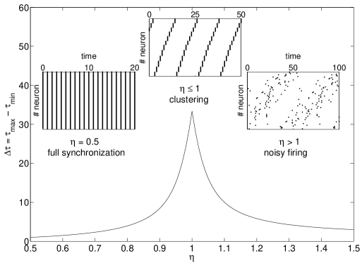
Figure 1: Number of possible ISIs according to the bound $\Delta\tau=\tau_{max}-\tau_{min}$ derived in [7]. For $\eta>1$ the network presents sub-critical behavior and is dominated by the noise. For $\eta<1$ it shows super-critical behavior. Criticality is produced at $\eta=1$, which coincides to the onset of sustained activity. At this point, the network is also broken down in a maximal number of clusters of units which fire according to a periodic pattern.

3 Self-organization using synaptic plasticity

We now introduce synaptic dynamics in the model. We first present the dissipated spontaneous evolution, a magnitude also maximized at $\eta=1$. The gradient of this magnitude turns to be simple analytically and leads to a plasticity rule that can be expressed using only local information encoded in the post-synaptic unit.

3.1 The dissipated spontaneous evolution

During one ISI, we distinguish between the spontaneous evolution carried out by a unit and the actual spontaneous evolution needed for a unit to reach the threshold $L$. The difference of both quantities can be regarded as a surplus of spontaneous evolution, which is dissipated during an ISI.

Figure 2a shows an example trajectory of a neuron’s state. First, we calculate the spontaneous evolution of the given unit during one ISI, which it is just its number of stochastic state transitions during an ISI of length $\tau$ (thick black lines in Figure 2a). These state transitions occur with probability $p$ at every timestep except from the timestep directly after spiking. Using the average ISI-length $\langle\tau\rangle$ over many spikes and all units we can calculate the average total spontaneous evolution:

$$E_{total} =(\langle\tau\rangle-1)p.$$ (4)

Since the state of a given unit can exceed the threshold because of the received messages from the rest of the population (blue dashed lines in Figure 2a), a fraction of (4) is actually not required to induce a spike in that unit, and therefore is dissipated. We can obtain this fraction by subtracting from (4) the actual number of state transitions that was required to reach the threshold $L$. The latter quantity can be referred to as effective spontaneous evolution $E_{eff}$ and is on average $L-1$ minus $(N-1)\langle\epsilon\rangle$, the mean evolution caused by the messages received from the rest of the units during an ISI. For $\eta\leq 1$, the activity is self-sustained and the messages from other units are enough to drive a unit above the threshold. In this case, all the spontaneous evolution is dissipated and $E_{eff}=0$. Summarizing, we have that:

$$E_{eff} =\max\{0,L-1-(N-1)\langle\epsilon\rangle\}=\begin{cases}L-1-(N-1)\langle\epsilon\rangle&\text{for $\eta\geq 1$}\\ 0&\text{for $\eta<1$}\end{cases}$$ (5)

If we subtract (5) from $E_{total}$ (4), we obtain the mean dissipated spontaneous evolution, which is visualized as red dimensioning in Figure 2a:

$$E_{diss} =E_{total}-E_{eff}=(\langle\tau\rangle-1)p-\max\{0,L-1-(N-1)\langle\epsilon\rangle\}.$$ (6)

Using (3) as an approximation of $\langle\tau\rangle$ we can get an analytic expression for $E_{diss}$.

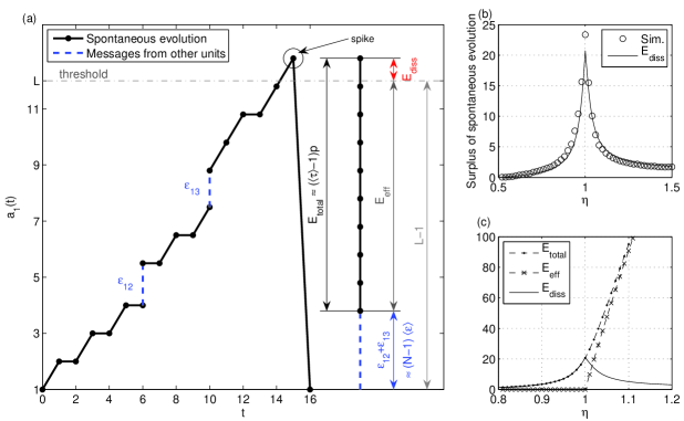
Figure 2: (a) Example trajectory of the state of a neuron: the dissipated spontaneous evolution $E_{diss}$ is the difference between the total spontaneous evolution $E_{total}$ (thick black lines) and the actual evolution required to reach the threshold $E_{eff}$ (dark gray dimensioning) in one ISI. (b) $E_{diss}$ is maximized at the critical point. (c) The three different evolutions involved in the analysis (parameters for (b) and (c) are $N=L=1000$ and $p=0.9$. For the mean ISI we used $\tau_{app}$ of Eq. (3)).

Figures 2b and c show this analytic curve $E_{diss}$ in function of $\eta$ together with the outcome of simulations.

At $\eta>1$ the units reach the threshold $L$ mainly because of their spontaneous evolution. Hence, $E_{total}\approx E_{eff}$ and $E_{diss}\approx 0$. The difference between $E_{total}$ and $E_{eff}$ increases as $\eta$ approaches $1$ because the message interchange progressively dominates the dynamics. At $\eta<1$, we have $E_{eff}=0$. In this scenario $E_{diss}=E_{total}$, is mainly determined by the ISI $\langle\tau\rangle$ and thus decays again for decreasing $\eta$. The maximum can be found at $\eta=1$.

3.2 Synaptic dynamics

After having presented our magnitude of interest we now derive a plasticity rule in the model. Our approach essentially assumes that updates of the individual synapses $\epsilon_{ij}$ are made in the direction of the gradient of $E_{diss}$. The analytical results are rather simple and allow a clear interpretation of the underlying mechanism governing the dynamics of the network under the proposed synaptic rule.

We start approximating the terms $N\langle\epsilon\rangle$ and $(N-1)\langle\epsilon\rangle$ by the sum of all pre-synaptic efficacies $\epsilon_{ik}$:

$$N\langle\epsilon\rangle=(N-1)\langle\epsilon\rangle+\langle\epsilon\rangle \approx(N-1)\langle\epsilon\rangle=\sum_{i=1}^{N}\sum_{k\neq i}{\epsilon_{ik}}/N\approx\sum_{k\neq i}{\epsilon_{ik}}.$$ (7)

This can be done for large $N$ and if we suppose that the distribution of $\epsilon_{ik}$ is the same for all $i$. $E_{diss}$ is now defined in terms of each individual neuron $i$ as:

$$E_{diss}^{i}=\left(\frac{L-1-\sum_{k\neq i}{\epsilon_{ik}}}{2p}+\sqrt{\left(\displaystyle\frac{L-1-\sum_{k\neq i}{\epsilon_{ik}}}{2p}+1\right)^{2}+\frac{\sum_{k\neq i}{\epsilon_{ik}}}{2p}}\right)p\\ -\max\{0,L-1-\sum_{k\neq i}{\epsilon_{ik}}\}.$$ (8)

An update of $\epsilon_{ij}$ occurs when a spike from the pre-synaptic unit $j$ induces a spike in a post-synaptic unit $i$. Other schedulings are also possible. The results are robust as long as synaptic updates are produced at the spike-time of the post-synaptic neuron.

$$\Delta\epsilon_{ij}=\kappa\frac{\partial{E^{i}_{diss}}}{\partial{\epsilon_{ij}}}=\kappa\left(\frac{\partial{E^{i}_{total}}}{\partial{\epsilon_{ij}}}-\frac{\partial E^{i}_{eff}}{\partial{\epsilon_{ij}}}\right),$$ (9)

where the constant $\kappa$ scales the amount of change in the synapse. We can write the gradient as:

$$\frac{\partial{E^{i}_{diss}}}{\partial{\epsilon_{ij}}}=\frac{-\frac{1}{2}\left(\frac{L-1-\sum_{k\neq i}{\epsilon_{ik}}}{2p}+\frac{1}{2}\right)}{\sqrt{\left(\frac{L-1-\sum_{k\neq i}{\epsilon_{ik}}}{2p}+1\right)^{2}+\frac{\sum_{k\neq i}{\epsilon_{ik}}}{2p}}}-\frac{1}{2}-\begin{cases}0&\text{if $(L-1-\sum_{k\neq i}{\epsilon_{ik}})<0$}\\ \text{indef}&\text{if $(L-1-\sum_{k\neq i}{\epsilon_{ik}})=0$}\\ -1&\text{if $(L-1-\sum_{k\neq i}{\epsilon_{ik}})>0$}.\end{cases}$$ (10)

For a plasticity rule to be biologically plausible it must be local, so only information encoded in the states of the pre-synaptic $j$ and the post-synaptic $i$ neurons must be considered to update $\epsilon_{ij}$.

We propagate $\sum_{k\neq i}{\epsilon_{ik}}$ to the state of the post-synaptic unit $i$ by considering for every unit $i$, an effective threshold $L^{i}$ which decreases deterministically every time an incoming pulse is received [6]. At the end of an ISI $L^{i}\approx(L-1-\sum_{k\neq i}{\epsilon_{ik}})$ and encodes implicitly all pre-synaptic efficacies of $i$. Intuitively, $L^{i}$ indicates how the activity received from the population in the last ISI differs from the activity required to induce and spike in $i$.

The only term involving non-local information in (10) is the noise rate $p$. We replace it by a constant $c$ and show later its limited influence on the synaptic rule. With these modifications we can write the derivative of $E^{i}_{diss}$ with respect to $\epsilon_{ij}$ as a function of only local terms:

$$\frac{\partial{E^{i}_{diss}}}{\partial{\epsilon_{ij}}} =\frac{-L^{i}-c}{2\sqrt{\left(L^{i}+2c\right)^{2}+2c(L-L^{i})}}+\frac{\text{sgn}(L^{i})}{2}$$ (11)

Note that, although the derivation based on the surplus spontaneous evolution (10) may involve information not locally accessible to the neuron, the derived rule (11) only requires a mechanism to keep track of the difference between the natural ISI and the actual one.

We can understand the mechanism involved in a particular synaptic update by analyzing in detail Eq. (11). In the case of a negative effective threshold ($L^{i}<0$) unit $i$ receives more input from the rest of the units than the required to spike, which translates into a weakening of the synapse. Conversely, if $L^{i}>0$ some spontaneous evolution was required for the unit $i$ to fire, Eq. (11) is positive and the synapse is strengthened. The intermediate case ($L^{i}=0$), corresponds to $\eta=1$ and no synaptic update is needed (nor is it defined). We will consider it thus $0$ for practical purposes.

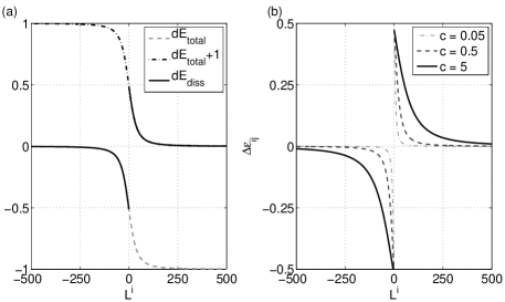
Figure 3: Plasticity rule. (a) First derivative of the dissipated spontaneous evolution $E_{diss}$ for $\kappa~{}=~{}1,L=1000$ and $c=0.9$. (b) The same rule for different values of $c$.

Figure 3a shows Eq. (11) in bold lines together with $\partial{E^{i}_{total}}/\partial{\epsilon_{ij}}$ (dashed line, corresponding to $\eta<1$) and $\partial{E^{i}_{total}}/\partial{\epsilon_{ij}}+1$ (dashed-dotted, $\eta>1$), for different values of the effective threshold $L^{i}$ of a given unit at the end on an ISI. $E_{total}$ indicates the amount of synaptic change and $E_{eff}$ determines whether the synapse is strengthened or weakened. The largest updates occur in the transition from a positive to a negative $L^{i}$ and tend to zero for larger absolute values of $L^{i}$. Therefore, significant updates correspond to those synapses with post-synaptic neurons which during the last ISI have received a similar amount of activity from the whole network as the one required to fire.

We remark the similarity between Figure 3b and the rule characterizing spike time dependent plasticity (STDP) [4, 13]. Although in STDP the change in the synaptic conductances is determined by the relative spike timing of the pre-synaptic neuron and the post-synaptic neuron and here it is determined by $L^{i}$ at the spiking time of the post-synaptic unit $i$, the largest changes in STDP occur also in an abrupt transition from strengthening to weakening corresponding to $L^{i}=0$ in Figure 3a.

Figure 3b illustrates the role of $c$ in the plasticity rule. For small $c$, updates are only significant in a tiny range of $L^{i}$ values near zero. For higher values of $c$, the interval of relevant updates is widened. The shape of the rule, however, is preserved, and the role of $c$ is just to scale the change in the synapse. For the rest of this manuscript, we will use $c=1$.

3.3 Simulations

In this section we show empirical results for the proposed plasticity rule. We focus our analysis on the time $\tau_{conv}$ required for the system to converge toward the critical point. In particular, we analyze how $\tau_{conv}$ depends on the starting initial configuration and on the constant $\kappa$.

For the experiments we use a network composed of $N=500$ units with homogeneous $L=500$ and $p=0.9$. Synapses are initialized homogeneously and random initial states are chosen for all units in each trial. Every time a unit $i$ fires, we update its afferent synapses $\epsilon_{ij}$, for all $j\neq i$, which breaks the homogeneity in the interaction strengths.

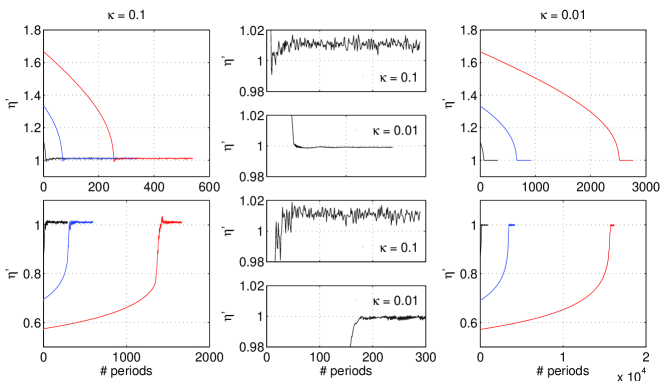
Figure 4: Empirical results of convergence toward $\eta=1$ for three different initial states above (top four plots) and below (bottom four plots) the critical point. Horizontal axis denote number of ISIs of the same random unit during all the simulations. On the left, results using the constant $\kappa=0.1$. Larger panels shows the full trajectory until $10^{3}$ timesteps after convergence. Smaller panels are a zoom of the first trajectory $\eta_{0}=1.1$ (top) and $\eta=0.87$ (bottom). Right panels show the same type of results but using a smaller constant $\kappa=0.01$.

The network starts with a certain initial condition $\eta_{0}$ and evolves according to its original discrete dynamics, Eq. (2), together with plasticity rule (9). To measure the time $\tau_{conv}$ necessary to reach a value close to $\eta=1$ for the first time, we select a neuron $i$ randomly and compute $\eta$ every time $i$ fires. We assume convergence when $\eta\in(1-\nu,1+\nu)$ for the first time. In these initial experiments, $\nu$ is set to $\kappa/5$ and $\kappa$ is either $0.1$ or $0.01$.

We performed $50$ random experiments for different initial configurations. In all cases, after an initial transient, the network settles close to $\eta=1$, presenting some fluctuations. These fluctuations did not grow even after $10^{6}$ ISIs in all realizations. Figure 4 shows examples for $\eta_{0}\in\{0.58,0.7,0.87,1.1,1.3,1.7\}$.

We can see that for larger updates of the synapses ($\kappa=0.1$) the network converges faster. However, fluctuations around the reached state, slightly above $\eta=1$, are approximately one order of magnitude bigger than for $\kappa=0.01$. We therefore can conclude that $\kappa$ determines the speed of convergence and the quality and stability of the dynamics at the critical state: high values of $\kappa$ cause fast convergence but turn the dynamics of the network less stable at the critical state.

We study now how $\tau_{conv}$ depends on $\eta_{0}$ in more detail. Given $N,L,c$ and $\kappa$, we can approximate the global change in $\eta$ after one entire ISI of a random unit assuming that all neurons change its afferent synapses uniformly. This gives us a recursive definition for the sequence of $\eta_{t}$s generated by the synaptic plasticity rule:

$$\Delta(\eta_{t}) =\kappa(N-1)\left(\frac{-L_{eff}(\eta_{t})-c}{2\sqrt{\left(L_{eff}(\eta_{t})+2c\right)^{2}+2c(L-L_{eff}(\eta_{t}))}}+\frac{\text{sgn}(\eta_{t}-1)}{2}\right),$$

$$\text{where }L_{eff}(\eta_{t})=(L-1)\left(1-\frac{1}{\eta_{t}}\right)\quad\text{ and }\quad\eta_{t+1}=\eta_{t}+\Delta(\eta_{t}).$$

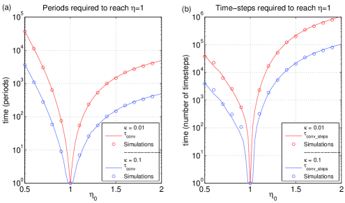
Figure 5: Number of ISIs (a) and timesteps (b) required to reach the critical state in function of the initial configuration $\eta_{0}$. Rounded dots indicate empirical results as averages over $10$ different realizations starting from the same $\eta_{0}$. Continuous curves correspond to Eq. (12). Parameter values are $N=500,L=500,p=0.9,c=1$, $\nu=\kappa/5$.

Then the number of ISIs and the number of timesteps can be obtained by:

$$\tau_{conv} =\text{min}(\{i:|\eta_{t}-1|\leq\nu\}), \tau_{conv\_steps} =\sum_{t=0}^{\tau_{conv}}\tau_{app}(\eta_{t}).$$ (12)

Figure 5 shows empirical values of $\tau_{conv}$ and $\tau_{conv\_steps}$ for several values of $\eta_{0}$ together with the approximations (12). Despite the inhomogeneous coupling strengths, the analytical approximations (continuous lines) of the experiments (circles) are quite accurate. Typically, for $\eta_{0}<1$ more spikes are required for convergence than for $\eta_{0}>1$. However, the opposite occurs if we consider timesteps as time units. A hysteresis effect (described in [7]) present in the system if $\eta_{0}<1$, causes the system to be more resistant against synaptic changes, which increases the number of updates (spikes) necessary to achieve the same effect as for $\eta_{0}>1$. Nevertheless, since the ISIs are much shorter for supercritical coupling the actual number of time steps is still lower than for subcritical coupling.

4 Discussion

Based on the amount of spontaneous evolution which is dissipated during an ISI, we have derived a local synaptic mechanism which causes a network of spiking neurons to self-organize near a critical state. Our motivation differs from those of similar studies, for instance [8], where the average branching ratio $\sigma$ of the network is used to characterize criticality. Briefly, $\sigma$ is defined as the average number of excitations created in the next time step by a spike of a given neuron.

The inverse of $\eta$ plays the role of the branching ratio $\sigma$ in our model. If we initialize the units uniformly in $[1,L]$, we have approximately one unit in every subinterval of length $\eta\epsilon$, and in consequence, the closest unit to the threshold spikes in $1/\eta$ cases if it receives a spike. For $\eta>1$, a spike of a neuron rarely induces another neuron to spike, so $\sigma<1$. Conversely, for $\eta<1$, the spike of a single neuron triggers more than one neuron to spike ($\sigma>1$). Only for $\eta=1$ the spike of a neuron elicits the order of one spike ($\sigma=1$). Our study thus represents a realization of a local synaptic mechanism which induces global homeostasis towards an optimal branching factor.

This idea is also related to the SOC rule proposed in [3], where a mechanism is defined for threshold gates (binary units) in terms of bit flip probabilities instead of spiking neurons. As in our model, criticality is achieved via synaptic scaling, where each neuron adjusts its synaptic input according to an effective threshold called margin.

When the network is operating at the critical regime, the dynamics can be seen as balancing between a predictable pattern of activity and uncorrelated random behavior typically present in SOC. One would also expect to find macroscopic magnitudes distributed according to scale-free distributions. Preliminary results indicate that, if the stochastic evolution is reset to zero ($p=0$) at the critical state, inducing an artificial spike on a randomly selected unit causes neuronal avalanches of sizes and lengths which span several orders of magnitude and follow heavy tailed distributions. These results are in concordance with what is usually found for SOC and will be published elsewhere.

The spontaneous evolution can be interpreted for instance as activity from other brain areas not considered in the pool of the simulated units, or as stochastic sensory input. Our results indicate that the amount of this stochastic activity that is absorbed by the system is maximized at an optimal state, which in a sense minimizes the possible effect of fluctuations due to noise on the behavior of the system.

The application of the synaptic rule for information processing is left for future research. We advance, however, that external perturbations when the network is critical would cause a transient activity. During the transient, synapses could be modified according to some other form of learning to encode the proper values which drive the whole network to attain a characteristic synchronized pattern for the external stimuli presented. We conjecture that the hysteresis effect shown in the regime of $\eta<1$ may be suitable for such purposes, since the network then is able to keep the same pattern of activity until the critical state is reached again.

Acknowledgments

We thank Joaquín J. Torres and Max Welling for useful suggestions and interesting discussions.

References

- [1] P. Bak. How nature works: The Science of Self-Organized Criticality. Springer, 1996.
- [2] J. M. Beggs and D. Plenz. Neuronal avalanches in neocortical circuits. Journal of Neuroscience, 23(35):11167–11177, December 2003.
- [3] N. Bertschinger, T. Natschläger, and R. A. Legenstein. At the edge of chaos: Real-time computations and self-organized criticality in recurrent neural networks. In Advances in Neural Information Processing Systems 17, pages 145–152. MIT Press, Cambridge, MA, 2005.
- [4] G. Q. Bi and M. M. Poo. Synaptic modifications in cultured hippocampal neurons: Dependence on spike timing, synaptic strength, and postsynaptic cell type. Journal Of Neuroscience, 18:10464–10472, 1998.
- [5] G. L. Gerstein and B. Mandelbrot. Random walk models for the spike activity of a single neuron. Biophys J., 4:41–68, 1964.
- [6] V. Gómez, A. Kaltenbrunner, and V. López. Event modeling of message interchange in stochastic neural ensembles. In IJCNN’06, Vancouver, BC, Canada, pages 81–88, 2006.
- [7] A. Kaltenbrunner, V. Gómez, and V. López. Phase transition and hysteresis in an ensemble of stochastic spiking neurons. Neural Computation, 19(11):3011–3050, 2007.
- [8] O. Kinouchi and M. Copelli. Optimal dynamical range of excitable networks at criticality. Nature Physics, 2:348, 2006.
- [9] C. G. Langton. Computation at the edge of chaos: Phase transitions and emergent computation. Physica D Nonlinear Phenomena, 42:12–37, jun 1990.
- [10] A. Levina, J. M. Herrmann, and T. Geisel. Dynamical synapses causing self-organized criticality in neural networks. Nature Physics, 3(12):857–860, 2007.
- [11] N. H. Packard. Adaptation toward the edge of chaos. In: Dynamics Patterns in Complex Systems, pages 293–301. World Scientific: Singapore, 1988. A. J. Mandell, J. A. S. Kelso, and M. F. Shlesinger, editors.
- [12] F. Rodríguez, A. Suárez, and V. López. Period focusing induced by network feedback in populations of noisy integrate-and-fire neurons. Neural Computation, 13(11):2495–2516, 2001.
- [13] S. Song, K. D. Miller, and L. F. Abbott. Competitive hebbian learning through spike-timing-dependent synaptic plasticity. Nature Neuroscience, 3(9):919–926, 2000.
- [14] G. G. Turrigiano and S. B. Nelson. Homeostatic plasticity in the developing nervous system. Nature Reviews Neuroscience, 5(2):97–107, 2004.
- [15] C. Van Vreeswijk and L. F. Abbott. Self-sustained firing in populations of integrate-and-fire neurons. SIAM J. Appl. Math., 53(1):253–264, 1993.