Nonlinear harmonic generation and devices in doubly-resonant Kerr cavities

Abstract

We describea theoretical analysis of the nonlinear dynamics of third-harmonic generation ($\omega\to 3\omega$) via Kerr ($\chi^{(3)}$) nonlinearities in a resonant cavity with resonances at both $\omega$ and $3\omega$. Such a doubly resonant cavity greatly reduces the required power for efficient harmonic generation, by a factor of $\sim V/Q^{2}$ where $V$ is the modal volume and $Q$ is the lifetime, and can even exhibit 100% harmonic conversion efficiency at a critical input power. However, we show that it also exhibits a rich variety of nonlinear dynamics, such as multistable solutions and long-period limit cycles.We describe how to compensate for self/cross-phase modulation (which otherwise shifts the cavity frequencies out of resonance), and how to excite the different stable solutions (and especially the high-efficiency solutions) by specially modulated input pulses.

I Introduction

In this paper, we describe how 100% third-harmonic conversion can occur in doubly-resonant optical cavities with Kerr nonlinearities, even when dynamical stability and self-phase modulation (which can drive the cavities out of resonance) are included (extending our earlier work Rodriguez07:OE ), and describe the initial conditions required to excite these efficient solutions. In particular, we show that such doubly-resonant nonlinear optical systems can display a rich variety of dynamical behaviors, including multistability (different steady states excited by varying initial conditions, a richer version of the bistable phenomenon observed in single-mode cavities Soljacic02:bistable ), long-period limit cycles (similar to the “self-pulsing” observed for second-harmonic generation Drummond80 ), and transitions in the stability and multiplicity of solutions as the parameters are varied. One reason for studying such doubly resonant cavities was the fact that they lower the power requirements for nonlinear devices Rodriguez07:OE , and in particular for third harmonic conversion, compared to singly-resonant cavities or nonresonant structures Armstrong62 ; Ashkin66 ; Smith70 ; Ferguson77 ; Brieger81 ; Berquist82 ; Kozlovsky88 ; Dixon89 ; Collet90 ; Persaud90 ; Moore95 ; Schneider96 ; Mu01 ; Hald01 ; McConnell01 ; Dolgova02 ; Liu05 ; Scaccabarozzi06 . An appreciation and understanding of these behaviors is important to design efficient harmonic converters (the main focus of this paper), but it also opens the possibility of new types of devices enabled by other aspects of the nonlinear dynamics.

In a Kerr ($\chi^{(3)}$) medium, there is a change in the refractive index proportional to the square of the electric field; for an oscillating field at a frequency $\omega$, this results in a shift in the index at the same frequency (self-phase modulation, SPM), generation of power at the third-harmonic frequency $3\omega$, and also other effects when multiple frequencies are present [cross-phase modulation (XPM) and four-wave mixing (FWM)] Boyd92 . When the field is confined in a cavity, restricting to a small modal volume $V$ for a long time given by the quality factor $Q$ (a lifetime in units of the optical period) JoannopoulosJo08-book , such nonlinear effects are enhanced by both the increased field strength for the same input power and by the frequency sensitivity inherent in resonant effects (since the fractional bandwidth is $1/Q$). This enhancement is exploited, for example, in nonlinear harmonic and sum-frequency generation, most commonly for $\chi^{(2)}$ effects where the change in index is proportional to the electric field (which requires a non-centrosymmetric material) Boyd92 . One can further enhance harmonic generation by using a cavity with two resonant modes, one at the source frequency and one at the harmonic frequency Paschotta94 ; Berger96 ; Zolotoverkh00 ; Maes05 ; Liscidini06 ; Dumeige06 ; Drummond80 ; Wu87 ; Ou93 . In this case, one must also take into account a nonlinear downconversion process that competes with harmonic generation Drummond80 ; Wu87 ; Ou93 , but it turns out to be theoretically possible to obtain 100% harmonic conversion for either $\chi^{(2)}$ ($\omega\to 2\omega$) or $\chi^{(3)}$ ($\omega\to 3\omega$) nonlinearities at a specific “critical” input power $P_{\mathrm{crit}}$ (both in a one-dimensional model of propagating waves for $\chi^{(2)}$ nonlinearities Schiller93:PhD and also in a more general coupled-mode model for either $\chi^{(2)}$ or $\chi^{(3)}$ nonlinearities Rodriguez07:OE ). In particular, we studied the harmonic-generation and downconversion processes in a broad class of model systems depicted in Fig. 1: a single input channel (e.g. a waveguide) is coupled to a nonlinear cavity with two resonant frequencies, where both reflected and harmonic fields are emitted back into the input channel. In this case, we predicted 100% harmonic generation at a critical power $P_{\mathrm{crit}}$ proportional to $V/Q^{3}$ for $\chi^{(2)}$ and $V/Q^{2}$ for $\chi^{(3)}$ Rodriguez07:OE . However, we only looked at the steady-state solution of the system and not its dynamics or stability. Moreover, in the $\chi^{(3)}$ case there can also be an SPM/XPM effect that shifts the cavity frequencies out of resonance and spoils the harmonic-generation effect. In this paper, we consider both of these effects, describe how to compensate for SPM/XPM, and demonstrate the different regimes of stability in such $\chi^{(3)}$ doubly resonant systems. We show that the parameters and the initial conditions must be chosen within certain regimes to obtain a stable steady state with high conversion efficiency.

In other regimes, we demonstrate radically different behaviors: not only low-efficiency steady states, but also limit-cycle solutions where the efficiency oscillates slowly with a repetition period of many thousands of optical cycles. With infrared light, these limit cycles form a kind of optical oscillator/clock with a period in the hundreds of GHz or THz (and possibly lower, depending on the cavity parameters). Previously, limit-cycle/self-pulsing behaviors have been observed in a number of other nonlinear optical systems, such as: doubly-resonant $\chi^{(2)}$ cavities coupled by second-harmonic generation Drummond80 ; bistable multimode Kerr cavities with time-delayed nonlinearities Abraham82 ; nonresonant distributed feedback in Bragg gratings Parini07 ; and a number of nonlinear lasing devices Siegman86 . However, the system considered in this work seems unusually simple, especially among $\chi^{(3)}$ systems, in that it only requires two modes and an instantaneous Kerr nonlinearity, with a constant-frequency input source, to attain self-pulsing, and partly as a consequence of this simplicity the precise self-pulsing solution is quite insensitive to the initial conditions. In other nonlinear optical systems where self-pulsing was observed, other authors have also observed chaotic solutions in certain regimes. Here, we did not observe chaos for any of the parameter regimes considered, where the input was a constant-frequency source, but it is possible that chaotic solutions may be excited by an appropriate pulsed input as in the $\chi^{(2)}$ case Drummond80 .

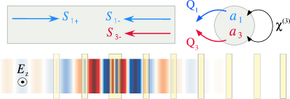
Figure 1: Top: Schematic of general scheme for third-harmonic generation, and dynamical variables for coupled-mode equations: a single input/output channel (with incoming/outgoing field amplitudes $s_{\pm}$) is coupled to a resonant cavity with two modes at frequencies $\omega_{1}$ and $3\omega_{1}$ (and corresponding amplitudes $a_{1}$ and $a_{3}$). The two resonant modes are nonlinearly coupled by a Kerr ($\chi^{(3)}$) nonlinearity. Bottom: An example realization Rodriguez07:OE , in one dimension, using a semi-infinite quarter-wave stack of dielectric layers with a doubled-layer defect (resonant cavity) that is coupled to incident plane waves; the electric field of a steady-state $3\omega_{1}$ solution is shown as blue/white/red for negative/zero/positive.

Another interesting phenomenon that can occur in nonlinear systems is multistability, where there are multiple possible steady-state solutions that one can switch among by varying the initial conditions. In Kerr ($\chi^{(3)}$) media, an important example of this phenomenon is bistable transmission through nonlinear cavities: for transmission through a single-mode cavity, output can switch discontinuously between a high-transmission and a low-transmission state in a hysteresis effect that results from SPM Soljacic02:bistable . For example, if one turns on the power gradually from zero the system stays in the low-transmission state, but if the power is increased further and then decreased to the original level, the system can be switched to the high-transmission state. This effect, which has been observed experimentally Notomi05 , can be used for all-optical logic, switching, rectification, and many other functions Soljacic02:bistable . In a cavity with multiple closely-spaced resonances, where the nonlinearity is strong enough to shift one cavity mode’s frequency to another’s, the same SPM phenomenon can lead to more than two stable solutions Felber76 . Here, we demonstrate a much richer variety of multistable phenomena in the doubly-resonant case for widely-separated cavity frequencies coupled by harmonic generation in addition to SPM—not only can there be more than two stable states, but the transitions between them can exhibit complicated oscillatory behaviors as the initial conditions are varied, and there are also Hopf bifurcations into self-pulsing solutions.

The remaining part of the paper is structured as follows. In Sec. II, we review the theoretical description of harmonic generation in a doubly resonant cavity coupled to input/output waveguides, based on temporal coupled-mode theory, and demonstrate the possibility of 100% harmonic conversion. We also discuss how to compensate for frequency shifting due to SPM and XPM by pre-shifting the cavity frequencies. In Sec. III, we analyze the stability of this 100%-efficiency solution, and demonstrate the different regimes of stable operation that are achieved in practice starting from that theoretical initial condition. We also present bifurcation diagrams that show how the stable and unstable solutions evolve as the parameters vary. Finally, in Sec. IV, we consider how to excite these high-efficiency solutions in practice, by examining the effect of varying initial conditions and uncertainties in the cavity parameters. In particular, we demonstrate the multistable phenomena exhibited as the initial conditions are varied. We close with some concluding remarks, discussing the many potential directions for future work that are revealed by the phenomena described here.

II 100% harmonic conversion in doubly-resonant cavities

In this section, we describe the basic theory of frequency conversion in doubly-resonant cavities with $\chi^{(3)}$ nonlinearities, including the undesirable self- and cross-phase modulation effects, and explain the existence of a solution with 100% harmonic conversion (without considering stability).

Consider a waveguide coupled to a doubly resonant cavity with two resonant frequencies $\omega_{1}^{\mathrm{cav}}=\omega_{1}$ and $\omega_{3}^{\mathrm{cav}}=\omega_{3}=3\omega_{1}$ (below, we will shift $\omega_{k}^{\mathrm{cav}}$ to differ slightly from $\omega_{k}$), and corresponding lifetimes $\tau_{1}$ and $\tau_{3}$ describing their radiation rates into the waveguide (or quality factors $Q_{k}=\omega_{k}\tau_{k}/2$). In addition, these modes are coupled to one another via the Kerr nonlinearity. Because all of these couplings are weak, any such system (regardless of the specific geometry), can be accurately described by temporal coupled-mode theory, in which the system is modeled as a set of coupled ordinary differential equations representing the amplitudes of the different modes, with coupling constants and frequencies determined by the specific geometry Suh04 ; Rodriguez07:OE . In particular, the coupled-mode equations for this particular class of geometries were derived in Rodriguez07:OE along with explicit equations for the coupling coefficients in a particular geometry. The degrees of freedom are the field amplitude $a_{k}$ of the $k$th cavity mode (normalized so that $|a_{k}|^{2}$ is the corresponding energy) and the field amplitude $s_{k\pm}$ of the incoming ($+$) and outgoing ($-$) waveguide modes at $\omega_{k}$ (normalized so that $|s_{k\pm}|^{2}$ is the corresponding power), as depicted schematically in Fig. 1. These field amplitudes are coupled by the following equations (assuming that there is only input at $\omega_{1}$, i.e. $s_{3+}=0$):

$$\begin{split}\dot{a_{1}}&=&\left[i\omega_{1}^{\mathrm{cav}}\left(1-\alpha_{11}|a_{1}|^{2}-\alpha_{13}|a_{3}|^{2}\right)-\frac{1}{\tau_{1}}\right]a_{1}\\ &&{}-i\omega_{1}\beta_{1}(a_{1}^{*})^{2}a_{3}+\sqrt{\frac{2}{\tau_{s,1}}}s_{1+}\end{split}$$ (1)

$$\begin{split}\dot{a_{3}}&=&\left[i\omega_{3}^{\mathrm{cav}}(1-\alpha_{31}|a_{1}|^{2}-\alpha_{33}|a_{3}|^{2})-\frac{1}{\tau_{3}}\right]a_{3}\\ &&{}-i\omega_{3}\beta_{3}a_{1}^{3}\end{split}$$ (2)

As explained in Rodriguez07:OE , the $\alpha$ and $\beta$ coefficients are geometry/material-dependent constants that express the strength of various nonlinear effects for the given modes. The $\alpha_{ij}$ terms describe self- and cross-phase modulation effects: they clearly give rise to effective frequency shifts in the two modes. The $\beta_{i}$ term characterize the energy transfer between the modes: the $\beta_{3}$ term describes frequency up-conversion and the $\beta_{1}$ term describes down-conversion. As shown in Rodriguez07:OE , they are related to one another via conservation of energy $\omega_{1}\beta_{1}=\omega_{3}\beta_{3}^{*}$, and all of the nonlinear coefficients scale inversely with the modal volume $V$.

There are three different $\alpha_{ij}$ parameters (two SPM coefficients $\alpha_{11}$ and $\alpha_{33}$ and one XPM coefficient $\alpha_{13}=\alpha_{31}$). All three values are different, in general, but are determined by similar integrals of the field patterns, produce similar frequency-shifting phenomena, and all scale as $1/V$. Therefore, in order to limit the parameter space analyzed in this paper, we consider the simplified case where all three frequency-shifting terms have the same strength $\alpha_{ij}=\alpha$.

One can also include various losses, e.g. linear losses correspond to a complex $\omega_{1}$ and/or $\omega_{3}$, and nonlinear two-photon absorption corresponds to a complex $\alpha$. As discussed in the concluding remarks, however, we have found that such considerations do not qualitatively change the results (only reducing the efficiency somewhat, as long as the losses are not too big compared to the radiative lifetimes $\tau$), and so in this manuscript we restrict ourselves to the idealized lossless case.

Figure 2 shows the steady-state conversion efficiency ($|s_{3-}|^{2}/|s_{1+}|^{2}$) versus input power of light that is incident on the cavity at $\omega^{cav}_{1}$, for the same parameter regime in Rodriguez07:OE (i.e. assuming negligible self- and cross-phase modulation so that $\alpha=0$), and not considering the stability of the steady state. As shown by the solid red curve, as one increases the input power, the efficiency increases, peaking at 100% conversion for a critical input power $P_{\mathrm{crit}}=|s_{1+}^{\mathrm{crit}}|$, where

$$|s_{1+}^{\mathrm{crit}}|=\left(\frac{4}{|\omega_{1}\beta_{1}|^{2}\tau_{1}^{3}\tau_{3}}\right)^{1/4}.$$ (3)

The efficiency decreases if the power is either too low (in the linear regime) or too high (dominated by down-conversion). $P_{\mathrm{crit}}$ scales as $V/Q^{2}$, so one can in principle obtain very low-power efficient harmonic conversion by increasing $Q$ and/or decreasing $V$ Rodriguez07:OE . Including absorption or other losses decreases the peak efficiency, but does not otherwise qualitatively change this solution Rodriguez07:OE .

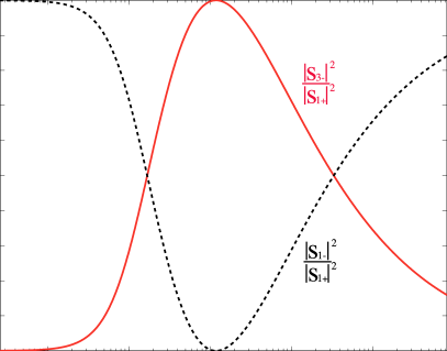
Figure 2: Steady-state efficiency of third-harmonic generation (solid red line) from Rodriguez07:OE , for $\alpha=0$ (no self-phase modulation), as a function of input power $|s_{1+}|^{2}$ scaled by the Kerr coefficient $n_{2}=3\chi^{(3)}/4c\varepsilon$. The reflected power at the incident frequency $\omega_{1}$ is shown as a dashed black line. There is a critical power where the efficiency of harmonic generation is 100. The parameters used in this plot are $Q_{1}=1000$, $Q_{3}=3000$, $\beta_{1}=(4.55985-0.7244i)\times 10^{-5}$ in dimensionless units of $\chi^{(3)}/V\epsilon$.

There are two effects that we did not previously analyze in detail, however, which can degrade this promising solution: nonlinear frequency shifts and instability. Here, we first consider frequency shifts, which arise whenever $\alpha\neq 0$, and consider stability in the next section. The problem with the $\alpha$ terms is that efficient harmonic conversion depends on the cavities being tuned to harmonic frequencies $\omega_{3}=3\omega_{1}$; a nonlinear shift in the cavity frequencies due to self/cross-phase modulation will spoil this resonance. In principle, there is a straightforward solution to this problem, as depicted in Fig. 3. Originally (for $\alpha=0$), the cavity was designed to have the frequency $\omega_{1}$ in the linear regime, but with $\alpha\neq 0$ the effective cavity frequency $\omega_{1}^{\mathrm{NL}}$ (including self/cross-phase modulation terms) is shifted away from the design frequency as shown by the blue line. Instead, we can simply design the linear cavity to have a frequency $\omega_{1}^{\mathrm{cav}}$ slightly different from the operating frequency $\omega_{1}$, so that self/cross-phase modulation shifts $\omega_{1}^{\mathrm{NL}}$ exactly to $\omega_{1}$ at the critical input power, as depicted by the green line in Fig. 3. Exactly the same strategy is used for $\omega_{3}^{\mathrm{NL}}$, by pre-shifting $\omega_{3}^{\mathrm{cav}}$.

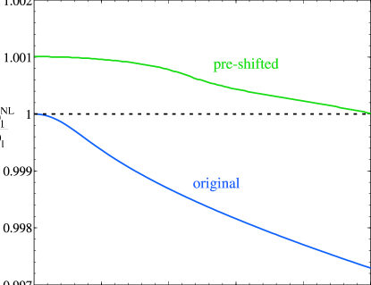
Figure 3: Shift in the resonant frequency $\omega_{1}^{\mathrm{NL}}$ as a function of input power, due to self/cross-phase modulation. (There is an identical shift in $\omega_{3}^{\mathrm{NL}}$.) If the cavity is designed so that the linear ($P_{\mathrm{in}}\to 0$) frequencies are harmonics, the nonlinearity pushes the system out of resonance (lower blue line) as the power increases to the critical power for 100% efficiency. This is corrected by pre-shifting the cavity frequencies (upper green line) so that the nonlinear frequency shift pushes the modes into resonance at $P_{\mathrm{crit}}$.

More precisely, to compute the required amount of pre-shifting, we examine the coupled-mode equations Eqs. (1–2). First, we solve for the critical power $P_{\mathrm{crit}}$ assuming $\alpha=0$, as in Rodriguez07:OE , and obtain the corresponding critical cavity fields $a_{k}^{\mathrm{crit}}$:

$$\left|a_{1}^{\mathrm{crit}}\right|^{2}=\left(\frac{1}{\omega_{1}^{2}\left|\beta_{1}\right|^{2}\tau_{3}\tau_{1,s}}\right)^{1/2}$$ (4)

$$\left|a_{3}^{\mathrm{crit}}\right|^{2}=\left(\frac{\omega_{3}\beta_{3}\tau_{3}}{(\omega_{1}\beta_{1}\tau_{1,s})^{3}}\right)^{1/2}.$$ (5)

Then, we substitute these critical fields into the coupled-mode equations for $\alpha\neq 0$, and solve for the new cavity frequencies $\omega_{k}^{\mathrm{cav}}$ so as to cancel the $\alpha$ terms and make the $a_{k}^{\mathrm{crit}}$ solutions still valid. This yields the following transformation of the cavity frequencies:

$$\omega_{1}^{\mathrm{cav}} =\frac{\omega_{1}}{1-\alpha_{11}|a_{1}^{\mathrm{crit}}|^{2}-\alpha_{13}|a_{3}^{\mathrm{crit}}|^{2}}$$ (6)

$$\omega_{3}^{\mathrm{cav}} =\frac{\omega_{3}}{1-\alpha_{13}|a_{1}^{\mathrm{crit}}|^{2}-\alpha_{33}|a_{3}^{\mathrm{crit}}|^{2}}.$$ (7)

By inspection, when substituted into Eqs. (1–2) at the critical power, these yield the same steady-state solution as for $\alpha=0$. (There are two other appearances of $\omega_{1}$ and $\omega_{3}$ in the coupled-mode equations, in the $\beta_{k}$ terms, but we need not change these frequencies because that is a higher-order effect, and the derivation of the coupled-mode equations considered only first-order terms in $\chi^{(3)}$.)

The nonlinear dynamics turn out to depend only on four dimensionless parameters: $\tau_{3}/\tau_{1}=Q_{3}/3Q_{1}$, $\alpha_{11}/\beta_{1}$, $\alpha_{33}/\beta_{1}$, and $\alpha_{13}/\beta_{1}=\alpha_{31}/\beta_{1}$. The overall scale of $Q$, $\alpha$, etcetera, merely determines the absolute scale for the power requirements: it is clear from the equations that multiplying all $\alpha$ and $\beta$ coefficients by an overall constant $K$ can be compensated by dividing all $a$ and $s$ amplitudes by $\sqrt{K}$ [which happens automatically for $s$ at the critical power by Eq. (3)]; the case of scaling $\tau_{1,3}$ by an overall constant is more subtle and is considered below. As mentioned above, for simplicity we take $\alpha_{11}=\alpha_{33}=\alpha_{13}=\alpha_{31}=\alpha$. Therefore, in the subsequent sections we will analyze the asymptotic efficiency as a function of $\tau_{3}/\tau_{1}$ and $\alpha/\beta_{1}$.

So far, we have found a steady-state solution to the coupled-mode equations, including self/cross-phase modulation, that achieves 100% third-harmonic conversion. In the following sections, we consider under what conditions this solution is stable, what other stable solutions exist, and for what initial conditions the high-efficiency solution is excited.

To understand the dynamics and stability of the nonlinear coupled-mode equations, we apply the standard technique of identifying fixed points of the equations and analyzing the stability of the linearized equations around each fixed point Tabor89 .

By a “fixed point,” we mean a steady-state solution corresponding to an input frequency $\omega_{1}$ ($s_{1+}\sim e^{-i\omega_{1}t}$) and hence $a_{1}(t)=A_{1}e^{-i\omega_{1}t}$ and $a_{3}(t)=A_{3}e^{-i3\omega_{1}t}$ for some unknown constants $A_{1}$ and $A_{3}$. [An input frequency $\omega_{1}$ can also generate higher harmonics, such as $9\omega_{1}$ or $5\omega_{1}$, but these are negligible: both because they are higher-order effects ($\sim[\chi^{(3)}]^{2}$, and all such terms were dropped in deriving the coupled-mode equations), and because we assume there is no resonant mode present at those frequencies.] By substituting this steady-state form into Eqs. (1–2), one obtains two coupled polynomial equations whose roots are the fixed points. We already know one of the fixed points from the previous section, the 100% efficiency solution, but to fully characterize the system one would like to know all of the fixed points (both stable and unstable). We solved these polynomial equations using Mathematica, which is able to compute all of the roots, but some transformations were required to put the equations into a solvable form. In particular, we eliminated the complex conjugations by writing $A_{k}=r_{k}e^{i\phi_{k}}$ and assuming (without loss of generality) that $s_{1+}$ is real. Multiplying Eq. (1) by $e^{-i\phi_{1}}$ and Eq. (2) by $e^{-i3\phi_{1}}$ allows us to simply solve the system for $e^{-i\phi_{1}}$ and $e^{i(\phi_{3}-3\phi_{1})}$. Requiring the magnitude of these two quantities to be unity yields two polynomials in $x=r_{1}^{2}$ and $y=r_{3}^{2}$, which Mathematica can handle. The resulting polynomial is of an artificially high degree, resulting in spurious roots, but the physical solutions are easily identified by the fact that $x$ and $y$ must be real and non-negative. (We should also note that this root-finding process is highly sensitive to roundoff error Press92 , independent of the physical stability of the solutions, but we dealt with that problem by employing 50 decimal places of precision.)

As mentioned above, the dynamics are independent of the overall scale of $\tau_{1,3}$, and depend only on the ratio $\tau_{3}/\tau_{1}$. This can be seen from the equations for $A_{1,3}$, in which the $\omega_{1,3}$ oscillation has been removed. In these equations, if we multiply $\tau_{1}$ and $\tau_{3}$ by an overall constant factor $K$, after some algebra it can be shown that the $A_{1,3}$ equations are invariant if we rescale $A_{1}\to A_{1}/\sqrt{K}$, $A_{3}\to A_{3}/\sqrt{K}$, rescale time $t\to Kt$, and rescale the input $s_{1+}\to s_{1+}/K$ [which happens automatically for the critical power by Eq. (3)]. Note also that the conversion efficiency $|s_{3-}/s_{1+}|^{2}=(2/\tau_{3})|A_{3}/s_{1+}|^{2}$ is also invariant under this rescaling by $K$. That is, the powers and the timescales of the dynamics change if you change the lifetimes, unsurprisingly, but the steady states, stability, etcetera (as investigated in the next section) are unaltered.

III Stability and dynamics

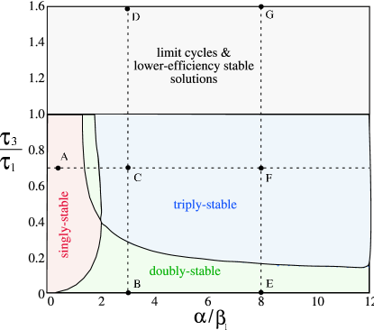
Figure 4: Phase diagram of the nonlinear dynamics of the doubly-resonant nonlinear harmonic generation system from Fig. 1 as a function of the relative cavity lifetimes ($\tau_{3}/\tau_{1}=3Q_{3}/Q_{1}$) and the relative strength of SPM/XPM vs. harmonic generation ($\alpha/\beta_{1}$) for input power equal to the critical power for 100% efficiency. For $\tau_{3}<\tau_{1}$ there is always one stable 100%-efficiency solution, and for nonzero $\alpha$ the system may have additional stable solutions. For $\tau_{3}>\tau_{1}$ the 100%-efficiency solution becomes unstable, but there are limit cycles and lower-efficiency stable solutions. Various typical points A–G in each region are labeled for reference in the subsequent figures.

Given the steady-state solutions (the roots), their stability is determined by linearizing the original equations around these points to a first-order linear equation of the form $d\mathbf{x}/dt=A\mathbf{x}$; a stable solution is one for which the eigenvalues of $A$ have negative real parts (leading to solutions that decay exponentially towards the fixed point) Tabor89 .

The results of this fixed-point and stability analysis are shown in Fig. 4 as a “phase diagram” of the system as a function of the relative lifetimes $\tau_{3}/\tau_{1}=3Q_{3}/Q_{1}$ and the relative strength of self-phase-modulation vs. four-wave mixing $\alpha/\beta_{1}$. Our original 100%-efficiency solution is always present, but is only stable for $\tau_{3}<\tau_{1}$ and becomes unstable for $\tau_{3}>\tau_{1}$. The transition point, $\tau_{3}=\tau_{1}$, corresponds to equal energy $|a_{1}|^{2}=|a_{3}|^{2}$ in the fundamental and harmonic mode at the critical input power. The unstable region corresponds to $|a_{3}|^{2}>|a_{1}|^{2}$ (and the down-conversion term is stronger than the up-conversion term)—intuitively, this solution is unstable because, if any perturbation causes the energy in the harmonic mode to decrease, there is not enough pumping from up-conversion to bring it back to the 100%-efficiency solution. Conversely, in the stable $|a_{3}|^{2}<|a_{1}|^{2}$ ($\tau_{3}<\tau_{1}$) regime, the higher-energy fundamental mode is being directly pumped by the input and can recover from perturbations. Furthermore, as $\alpha/\beta_{1}$ increases, additional lower-efficiency stable solutions are introduced, resulting in regimes with two (doubly stable) and three (triply stable) stable fixed points. These different regimes are explored in more detail via bifurcation diagrams below, and the excitation of the different stable solutions is considered in the next section.

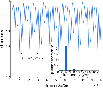
Figure 5: An example of a limit-cycle solution, with a periodically oscillating harmonic-generation efficiency as a function of time, corresponding to point D in Fig. 4. Perturbations in the initial conditions produce only phase shifts in the asymptotic cycle. Here, the limit cycle has a period of around $3\times 10^{4}$ optical cycles. Inset: Square of Fourier amplitudes (arbitary units) for each harmonic component of the limit cycle in the Fourier-series expansion of the $|A_{3}|$.

For $\tau_{3}>\tau_{1}$, the 100%-efficiency solution is unstable, but there are lower-efficiency steady-state solutions and also another interesting phenomenon: limit cycles. A limit cycle is a stable oscillating-efficiency solution, one example of which (corresponding to point D in Fig. 4) is plotted as a function time in Fig. 5. (In general, the existence of limit cycles is difficult to establish analytically Tabor89 , but the phenomenon is clear in the numerical solutions as a periodic oscillation insensitive to the initial conditions). In fact, as we shall see below, these limit cycles result from a “Hopf bifurcation,” which is a transition from a stable fixed point to an unstable fixed point and a limit cycle Strogatz94 . In this example at point D, the efficiency oscillates between roughly 66% and nearly 100%, with a period of several thousand optical cycles. As a consequence of the time sacling described in the last paragraph of the previous section, the period of such limit cycles is proportional to the $\tau$’s. If the frequency $\omega_{1}$ were $1.55\,\mu$m, for a $Q_{1}$ of $500$ optical cycles, this limit cycle would have a frequency of around $70$ GHz, forming an interesting type of optical “clock” or oscillator. Furthermore, the oscillation is not sinusoidal and contains several higher harmonics as shown in the inset of Fig. 5; the dominant frequency component in this case is the fourth harmonic ($\sim 280$ GHz), but different points in the phase diagram yield limit cycles with different balances of Fourier components.

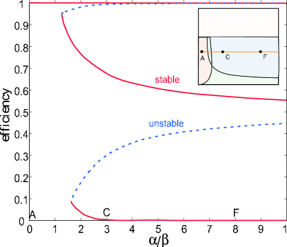
Figure 6: Bifurcation diagram showing the harmonic-generation efficiency of the stable (solid red lines) and unstable (dashed blue lines) steady-state solutions as a function of $\alpha/\beta_{1}$ for a fixed $\tau_{3}/\tau_{1}=0.7$, corresponding to the line ACF in Fig. 4 (see inset). The input power is the critical power $P_{\mathrm{crit}}$, so there is always a 100%-efficiency stable solution, but as $\alpha/\beta_{1}$ increases new stable and unstable solutions appear at lower efficiencies.

To better understand the phase diagram of Fig. 4, it is useful to plot the efficiencies of both the stable and unstable solutions as a function of various parameters. Several of these bifurcation diagrams (in which new fixed points typically appear in stable/unstable pairs) are shown in Figs. 6–8. To begin with, Figs. 6 and 7 correspond to lines connecting the labeled points ACF, BCD, and ECG, respectively, in Fig. 4, showing how the stability changes as a function of $\alpha/\beta_{1}$ and $\tau_{3}/\tau_{1}$. Figure 6 shows how first one then two new stable fixed points appear as $\alpha/\beta_{1}$ is increased, one approaching zero efficiency and the other closer to 50%. Along with these two stable solutions appear two unstable solutions (dashed lines). (A similar looking plot, albeit inverted, can be found in Felber76 for SPM-coupled closely-spaced resonances.) In particular, the fact that one of the unstable solutions approaches the 100%-efficiency stable solution causes the latter to have a smaller and smaller basin of attraction as $\alpha/\beta_{1}$ increases, making it harder to excite as described in the next section. The next two plots, in Fig. 7, both show the solutions with respect to changes in $\tau_{3}/\tau_{1}$ at two different values of $\alpha/\beta_{1}$. They demonstrate that at $\tau_{1}=\tau_{3}$, a Hopf bifurcation occurs where the 100%-efficiency solution becomes unstable for $\tau_{3}\geq\tau_{1}$ and limit cycles appear, intuitively seeming to “bounce between” the two nearby unstable fixed points. (The actual phase space is higher dimensional, however, so the limit cycles are not constrained to lie strictly between the efficiencies of the two unstable solutions.) It is worth to note that the remaining nonzero-efficiency stable solution (which appears at a nonzero $\tau_{3}/\tau_{1}$) becomes less efficient as $\tau_{3}/\tau_{1}$ increases.

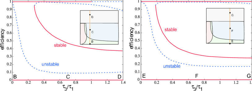
Figure 7: Bifurcation diagram showing the harmonic-generation efficiency of the stable (solid red lines) and unstable (dashed blue lines) steady-state solutions as a function of $\tau_{3}/\tau_{1}$ for a fixed $\alpha/\beta_{1}=3$ (left) or $=8$ (right), corresponding to the lines BCD or EFG, respectively, in Fig. 4 (see insets). The input power is the critical power $P_{\mathrm{crit}}$, so there is always a 100%-efficiency steady-state solution, but it becomes unstable for $\tau_{3}>\tau_{1}$ (a Hopf bifurcation leading to limit cycles as in Fig. 5).

The above analysis and results were for the steady-state-solutions when operating at the critical input power to obtain a 100%-efficiency solution. However, one can, of course, operate with a different input power—although no other input power will yield a 100%-efficient steady-state solution, different input powers may still be useful because (as noted above and in the next section) the 100%-efficiency solution may be unstable or practically unattainable. Figure 8(left) is the bifurcation diagram with respect to the input power $P_{\mathrm{in}}/P_{\mathrm{crit}}$ at fixed $\alpha/\beta_{1}$ and fixed $\tau_{3}/\tau_{1}$, corresponding to point C in Fig. 4. This power bifurcation diagram displays a number of interesting features, with the steady-state solutions transitioning several times from stable to unstable and vice versa. As we will see in the next section, the stability transitions in the uppermost branch are actually supercritical (reversible) Hopf bifurcations to/from limit cycles. Near the critical power, there is only a small region of stability of the near-100%-efficiency solution, as shown in the inset of Fig. 8(left). In contrast, the lower-efficiency stable solutions have much larger stable regions of the curve while still maintaining efficiencies greater than 70% at low powers comparable to $P_{\mathrm{crit}}\sim V/Q^{2}$, which suggests that they may be attractive regimes for practical operation when $\alpha/\beta_{1}$ is not small. This is further explored in the next section, and also by Fig. 8(right) which shows the bifurcation diagram along the line ACF in Fig. 4 [similar to Fig. 6], but at 135% of the critical input power. For this higher power, the system becomes at most doubly stable as $\alpha/\beta_{1}$ is increased, and the higher-efficiency stable solution becomes surprisingly close to 100% as $\alpha/\beta_{1}\to 0$.

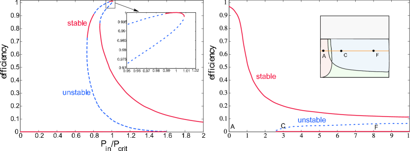
Figure 8: Left: Bifurcation diagram showing the harmonic-generation efficiency of the stable (solid red lines) and unstable (dashed blue lines) steady-state solutions as a function of input power $P_{\mathrm{in}}/P_{\mathrm{crit}}$ at fixed $\alpha/\beta_{1}=3$ and $\tau_{3}/\tau_{1}=0.7$, corresponding to point C in Fig. 4; the inset shows an enlarged view of the high-efficiency solutions. Right: Bifurcation diagram as a function of $\alpha/\beta_{1}$ for fixed $P_{\mathrm{in}}/P_{\mathrm{crit}}=1.35$ and fixed $\tau_{3}/\tau_{1}=0.7$; in this case, because it is not at the critical power, there are no 100%-efficiency solutions.

IV Exciting high-efficiency solutions

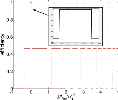
Figure 9: Asymptotic steady-state efficiency at point C (triply-stable) in the phase diagram (Fig. 4), with the initial conditions perturbed from the 100%-efficiency stable solution. The initial amplitudes $A_{10}$ and $A_{30}$ are perturbed by $\delta A_{10}$ and $\delta A_{30}$, respectively, with $\delta A_{10}/A_{1}^{\mathrm{crit}}=\delta A_{30}/A_{3}^{\mathrm{crit}}$. The oscillation of the steady-state efficiency with the perturbation strength is an indication of the complexity of the phase space and the shapes of the basins of attraction of each fixed point.

One remaining concern in any multistable system is how to excite the desired solution—depending on the initial conditions, the system may fall into different stable solutions, and simply turning on the source at the critical input power may result in an undesired low-efficiency solution. If $\alpha/\beta$ is small enough, of course, then from Fig. 4 the high-efficiency solution is the only stable solution and the system must inevitably end up in this state no matter how the critical power is turned on. Many interesting physical systems will correspond to larger values of $\alpha/\beta$, however Rodriguez07:OE , and in this case the excitation problem is complicated by the existence of other stable solutions. Moreover, the basins of attraction of each stable solution may be very complicated in the phase space, as illustrated by Fig. 9, where varying the initial cavity amplitudes $A_{1,3}$ from the 100%-efficiency solution causes the steady state to oscillate in a complicated way between the three stable solutions (at point C in Fig. 4). We have investigated several solutions to this excitation problem, and found an “adiabatic” excitation technique that reliably produces the high-efficiency solution without unreasonable sensitivity to the precise excitation conditions.

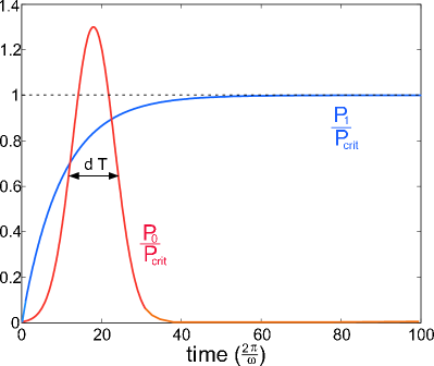
Figure 10: One way of exciting the system into a controlled stable solution: the input power is the sum of an exponential turn-on (the blue curve, $P_{1}$) and a Gaussian pulse with amplitude $P_{0}$ and width $\delta T$. The amplitude $P_{0}$ is altered to control which stable solution the system ends up in.

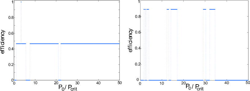
Figure 11: Left: Steady-state efficiency at point C in Fig. 4 as a function of the transient input-pulse power $P_{0}$ from Fig. 10, showing how all three stable solutions can be excited by an appropriate input-pulse amplitude. Right: Same, but for an asymptotic input power $P_{1}\approx 0.8P_{\mathrm{crit}}$, for which the maximum efficiency is $\approx 90\%$ from Fig. 8(right), but is easier to excite.

First, we considered a simple technique similar to the one described in Soljacic02:bistable for exciting different solutions of a bistable filter: as shown in Fig. 10, we “turn on” the input power by superimposing a gradual exponential turn-on (asymptoting to $P_{1}=P_{\mathrm{crit}}$) with a Gaussian pulse of amplitude $P_{0}$ and width $\delta T$. The function of the initial pulse is to “kick” the system into the desired stable solution. We computed the eventual steady-state efficiency (after all transient effects have disappeared) as a function of the pulse amplitude $P_{0}$ at point C in Fig. 4, where there are three stable solutions. The results are shown in Fig. 11(left), and indeed we see that all three stable solutions from point C in Fig. 6: one at near-zero efficiency, one at around 47% efficiency, and one at 100% efficiency. Unfortunately, the 100% efficiency solution is obviously rather difficult to excite, since it occurs for only a very narrow range of $P_{0}$ values. One approach to dealing with this challenge is to relax the requirement of 100% efficiency (which will never be obtained in practice anyway due to losses), and operate at a power $P_{1}<P_{\mathrm{crit}}$. In particular, Fig. 8(left) shows that there is a much larger stable region for $P_{1}\approx 0.8P_{\mathrm{crit}}$ with efficiency around 90%, leading one to suspect that this solution may be easier to excite than the 100%-efficiency solution at $P_{1}=P_{\mathrm{crit}}$. This is indeed the case, as is shown in Fig. 11(right), plotting efficiency vs. $P_{0}$ at point C with $P_{1}\approx 0.8P_{\mathrm{crit}}$. In this case, there are only two stable solutions, consistent with Fig. 8(left), and there are much wider ranges of $P_{0}$ that attain the high-efficiency ($\approx 90\%$) solution.

There are also many other ways to excite the high-efficiency solution (or whatever steady-state solution is desired). For example, because the cavity is initially detuned from the input frequency, as described in Sec. II, much of the initial pulse power is actually reflected during the transient period, and a more efficient solution would vary the pulse frequency in time to match the cavity frequency as it detunes. One can also, of course, vary the initial pulse width or shape, and by optimizing the pulse shape one may obtain a more robust solution.

In particular, one can devise a different (constant-frequency) input pulse shape that robustly excites the high-efficiency solution, insensitive to small changes in the initial conditions, by examining the power-bifurcation diagram in Fig. 8(left) in more detail. First, we observe that input powers $\gtrsim 1.45P_{\mathrm{crit}}$ have only one stable solution, meaning that this stable solution is excited regardless of the initial conditions or the manner in which the input power is turned on. Then, if we slowly decrease the input power, the solution must “adiabatically” follow this stable solution in the bifurcation diagram until a power $\approx 0.95P_{\mathrm{crit}}$ is reached, at which point that stable solution disappears. In fact, by inspection of Fig. 8(left), at that point there are no stable solutions, and solution jumps into a limit cycle. If the power is further decreased, a high-efficiency stable solution reappears and the system must drop into this steady state (being the only stable solution at that point). This process of gradually decreasing the power is depicted in Fig. 12(left), where the instantaneous “efficiency” is plotted as a function of input power, as the input power is slowly decreased. (The efficiency can exceed unity,because we are plotting instantaneous output vs. input power, and in the limit-cycle self-pulsing solution the output power is concentrated into pulses whose peak can naturally exceed the average input or output power.) Already, this is an attractive way to excite a high-efficiency ($>90\%$) solution, because it is insensitive to the precise manner in which we change the power as long as it is changed slowly enough—this rate is determined by the lifetime of the cavity, and since this lifetime is likely to be sub-nanosecond in practice, it is not difficult to change the power “slowly” on that timescale. However, we can do even better, once we attain this high-efficiency steady state, by then increasing the power adiabatically. As we increase the power, starting from the high-efficiency steady-state solution below the critical power, the system first enters limit-cycle solutions when the power becomes large enough that the stable solution disappears in Fig. 8(left). As we increase the power further, however, we observe that these limit cycles always converge adiabatically into the 100%-efficiency solution when $P\to P_{\mathrm{crit}}$. This process is shown in Fig. 12(right). What is happening is actually a supercritical Hopf bifurcation at the two points where the upper branch changes between stable and unstable: this is a reversible transition between a stable solution and a limit cycle (initially small oscillations, growing larger and larger away from the transition). This is precisely what we observe in Fig. 12, in which the limit cycle amplitudes become smaller and smaller as the stable solutions on either side of the upper branch are approached, leading to the observed reversible transitions between the two. The important fact is that, in this way, by first decreasing and then increasing the power to $P_{\mathrm{crit}}$, one always obtains the 100%-efficiency solution regardless of the precise details of how the power is varied (as long as it is “slow” on the timescale of the cavity lifetime).

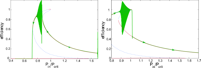
Figure 12: Left: Black line with arrows indicates instantaneous “efficiency” (harmonic output power / input power) as the input power is slowly decreased, starting at a power $\approx 1.7P_{\mathrm{crit}}$. For comparison, Fig. 8(left) is superimposed as solid-red and dashed-blue lines. The solution “adiabatically” follows a steady state until the steady state becomes unstable, at which point it enters limit cycles, and then returns to a high-efficiency steady state, and finally goes drops to a low-efficiency steady-state if the power is further decreased. Right: Similar, but here the power is increased starting at the high-efficiency steady state solution for $P<P_{\mathrm{crit}}$. In this case, it again enters limit cycles, but then it returns to a high-efficiency steady-state solution as the power is further increased, eventually reaching the 100%-efficiency stable solution. If the power is further increased, it drops discontinuously to the remaining lower-efficiency steady-state stable solution.

V Concluding Remarks

We have shown that a doubly-resonant cavity not only has high-efficiency harmonic conversion solutions for low input power, as in our previous work Rodriguez07:OE , but also exhibits a number of other interesting phenomena. We showed under what conditions the high-efficiency solution is stable, how to compensate for self-phase modulation, the existence of different regimes of multistable solutions and limit cycles controlled by the parameters of the system and by the input power, and how to excite the desired high-efficiency solution. Although we did not observe chaos, it seems possible that this may be obtained in future work for other parameter regimes, e.g. for pulsed input power as was observed in the $\chi^{(2)}$ case Drummond80 . These dynamical phenomena depend only on certain dimensionless quantities $\alpha/\beta$, $\omega_{3}/\omega_{1}$, $\tau_{3}/\tau_{1}$, and $s_{1+}/s_{1+}^{\mathrm{crit}}$, although the overall power and time scales depend upon the dimensionful quantities $\tau_{1,3}$ and so on.

All of the calculations in this paper were for an idealized lossless system, as our main intention was to examine the fundamental dynamics of these systems rather than a specific experimental realization. However, we have performed preliminary calculations including both linear losses (such as radiation or material absorption) and nonlinear two-photon absorption, and we find that these losses do not qualitatively change the observed phenomena. One still obtains multistability, limit cycles, bifurcations, and so on, merely at reduced peak efficiency depending on the strength of the losses. In a future manuscript, we plan to explore these effects in more detail in realistic material settings, and propose specific geometries to obtain the requisite doubly-resonant cavities. In particular, to obtain widely-spaced resonant modes $\omega$ and $3\omega$ in a nanophotonic (wavelength-scale) context (as opposed to macroscopic Fabry-Perot cavities with mirrors), the most promising route seems to be a ring resonator of some sort Saleh91 , rather than a photonic crystal JoannopoulosJo08-book (since photonic band gaps at widely separated frequencies are difficult to obtain in two or three dimensions). Although such a cavity will naturally support more than the two $\omega_{1}$ and $\omega_{3}$ modes, only two of the modes will be properly tuned to achieve the resonance condition for strong nonlinear coupling.

Finally, we should mention that similar phenomena should also arise in doubly and triply resonant cavities coupled nonlinearly by sum/difference frequency generation (for $\chi^{(2)}$) or four-wave mixing (for $\chi^{(3)}$). The advantage of this is that the coupled frequencies can lie closer together, imposing less stringent materials constraints and allowing the cavity to be confined by narrow-bandwidth mechanisms such as photonic band gaps JoannopoulosJo08-book , at the cost of a more complicated cavity design.

References

- (1) A. Rodriguez, M. Soljačić, J. D. Joannopulos, and S. G. Johnson, “ and harmonic generation at a critical power in inhomogeneous doubly resonant cavities,” Opt. Express, vol. 15, no. 12, pp. 7303–7318, 2007.
- (2) M. Soljačić, M. Ibanescu, S. G. Johnson, Y. Fink, and J. D. Joannopoulos, “Optimal bistable switching in non-linear photonic crystals,” Phys. Rev. E Rapid Commun., vol. 66, p. 055601(R), 2002.
- (3) P. D. Drummond, K. J. McNeil, and D. F. Walls, “Non-equilibrium transitions in sub/second harmonic generation i: Semiclassical theory,” Optica Acta., vol. 27, no. 3, pp. 321–335, 1980.
- (4) J. A. Armstrong, N. loembergen, J. Ducuing, and P. S. Pershan, “Interactions between light waves in a nonlinear dielectric,” Phys. Rev., vol. 127, pp. 1918–1939, 1962.
- (5) A. Ashkin, G. D. Boyd, and J. M. Dziedzic, “Resonant optical second harmonic generation and mixing,” IEEE J. Quantum Electron., vol. 2, pp. 109–124, 1966.
- (6) R. G. Smith, “Theory of intracavity optical second-harmonic generation,” IEEE J. Quantum Electron., vol. 6, pp. 215–223, 1970.
- (7) A. I. Gerguson and M. H. Dunn, “Intracavity second harmonic generation in continuous-wave dye lasers,” IEEE J. Quantum Electron., vol. 13, pp. 751–756, 1977.
- (8) M. Brieger, H. Busener, A. Hese, F. V. Moers, and A. Renn, “Enhancement of single frequency shg in a passive ring resonator,” Opt. Commun., vol. 38, pp. 423–426, 1981.
- (9) J. C. Berquist, H. Hemmati, and W. M. Itano, “High power second harmonic generation of 257 nm radiation in an external ring cavity,” Opt. Commun., vol. 43, pp. 437–442, 1982.
- (10) W. J. Kozlovsky, W. P. Risk, W. Lenth, B. G. Kim, G. L. Bona, H. Jaeckel, and D. J. Webb, “Blue light generation by resonator-enhanced frequency doubling of an extended-cavity diode laser,” Appl. Phys. Lett., vol. 65, pp. 525–527, 1994.
- (11) G. J. Dixon, C. E. Tanner, and C. E. Wieman, “432-nm source based on efficient second-harmonic generation of gaalas diode-laser radiation in a self-locking external resonant cavity,” Opt. Lett., vol. 14, pp. 731–733, 1989.
- (12) M. J. Collet and R. B. Levien, “Two-photon loss model of intracavity second-harmonic generation,” Phys. Rev. A, vol. 43, no. 9, pp. 5068–5073, 1990.
- (13) M. A. Persaud, J. M. Tolchard, and A. I. Ferguson, “Efficient generation of picosecond pulses at 243 nm,” IEEE J. Quantum Electron., vol. 26, pp. 1253–1258, 1990.
- (14) G. T. Moore, K. Koch, and E. C. Cheung, “Optical parametric oscillation with intracavity second-harmonic generation,” Optics Communications, vol. 113, p. 463, 1995.
- (15) K. Schneider, S. Schiller, and J. Mlynek, “1.1-w single-frequency 532-nm radiation by second-harmonic generation of a miniature nd:yag ring laser,” Opt. Lett., vol. 21, pp. 1999–2001, 1996.
- (16) X. Mu, Y. J. Ding, H. Yang, and G. J. Salamo, “Cavity-enhanced and quasiphase-matched mutli-order reflection-second-harmonic generation from gaas/alas and gaas/algaas multilayers,” Appl. Phys. Lett., vol. 79, p. 569, 2001.
- (17) J. Hald, “Second harmonic generation in an external ring cavity with a brewster-cut nonlinear cystal: theoretical considerations,” Optics Communications, vol. 197, p. 169, 2001.
- (18) G. McConnell, A. I. Ferguson, and N. Langford, “Cavity-augmented frequency tripling of a continuous wave mode-locked laser,” J. Phys. D: Appl.Phys, vol. 34, p. 2408, 2001.
- (19) T. V. Dolgova, A. I. Maidykovski, M. G. Martemyanov, A. A. Fedyanin, O. A. Aktsipetrov, G. Marowsky, V. A. Yakovlev, G. Mattei, N. Ohta, and S. Nakabayashi, “Giant optical second-harmonic generation in single and coupled microcavities formed from one-dimensional photonic crystals,” J. Opt. Soc. Am. B, vol. 19, p. 2129, 2002.
- (20) T.-M. Liu, C.-T. Yu, and C.-K. Sun, “2 ghz repetition-rate femtosecond blue sources by second-harmonic generation in a resonantly enhanced cavity,” Appl. Phys. Lett., vol. 86, p. 061112, 2005.
- (21) L. Scaccabarozzi, M. M. Fejer, Y. Huo, S. Fan, X. Yu, and J. S. Harris, “Enchanced second-harmonic generation in algaas/alxoy tightly confining waveguides and resonant cavities,” OL, vol. 31, no. 24, pp. 3626–3630, 2006.
- (22) R. W. Boyd, Nonlinear Optics. California: Academic Press, 1992.
- (23) J. D. Joannopoulos, S. G. Johnson, J. N. Winn, and R. D. Meade, Photonic Crystals: Molding the Flow of Light. Princeton University Press, second ed., February 2008.
- (24) R. Paschotta, K. Fiedler, P. Kurz, and J. Mlynek, “Nonlinear mode coupling in doubly resonant frequency doublers,” Appl. Phys. Lett., vol. 58, p. 117, 1994.
- (25) V. Berger, “Second-harmonic generation in monolithic cavities,” J. Opt. Soc. Am. B, vol. 14, p. 1351, 1997.
- (26) I. I. Zootoverkh, K. N. V., and E. G. Lariontsev, “Enhancement of the efficiency of second-harmonic generation in microlaser,” Quantum Electronics, vol. 30, p. 565, 2000.
- (27) B. Maes, P. Bienstman, and R. Baets, “Modeling second-harmonic generation by use of mode expansion,” J. Opt. Soc. Am. B, vol. 22, p. 1378, 2005.
- (28) M. Liscidini and L. A. Andreani, “Second-harmonic generation in doubly resonant microcavities with periodic dielectric mirrors,” Phys. Rev. E, vol. 73, p. 016613, 2006.
- (29) Y. Dumeige and P. Feron, “Wispering-gallery-mode analysis of phase-matched doubly resonant second-harmonic generation,” Phys. Rev. A, vol. 74, p. 063804, 2006.
- (30) L.-A. Wu, M. Xiao, and H. J. Kimble, “Squeezed states of light from an optical parametric oscillator,” JOSA-B, vol. 4, pp. 1465–1476, 1987.
- (31) Z. Y. Ou and H. J. Kimble, “Enhanced conversion efficiency for harmonic generation with double resonance,” Opt. Lett., vol. 18, pp. 1053–1055, 1993.
- (32) S. Schiller, Principles and Applications of Optical Monolithic Total-Internal-Reflection Resonators. PhD thesis, Stanford University, Stanford, CA, March 1993.
- (33) E. Abraham, W. J. Firth, and J. Carr, “Self-oscillation and chaos in nonlinear Fabry-Perot resonators with finite response time,” Physics Lett. A, pp. 47–51, 1982.
- (34) A. Parini, G. Bellanca, S. Trillo, M. Conforti, A. Locatelli, and C. De Angelis, “Self-pulsing and bistability in nonlinear Bragg gratings,” J. Opt. Soc. Am. B, vol. 24, pp. 2229–2237, 2007.
- (35) A. Siegman, Lasers. Mill Valley, CA: University Science Books, 1986.
- (36) M. Notomi, A. Shinya, S. Mitsugi, G. Kira, E. Kuramochi, and T. Tanabe, “Optical bistable switching action of Si high- photonic-crystal nanocavities,” Opt. Express, vol. 13, no. 7, pp. 2678–2687, 2005.
- (37) F. S. Felber and J. H. Marburger, “Theory of nonresonant multistable optical devices,” Appl. Phys. Lett., vol. 28, no. 12, pp. 731–733, 1976.
- (38) W. Suh, Z. Wang, and S. Fan, “Temporal coupled-mode theory and the presence of non-orthogonal modes in lossless multimode cavities,” IEEE J. Quantum Electron., vol. 40, no. 10, pp. 1511–1518, 2004.
- (39) M. Tabor, Chaos and Integrability in Nonlinear Dynamics: An Introduction. New York: Wiley, 1989.
- (40) W. H. Press, S. A. Teukolsky, W. T. Vetterling, and B. P. Flannery, Numerical Recipes in C: The Art of Scientific Computing. Cambridge Univ. Press, second ed., 1992.
- (41) S. H. Strogatz, Nonlinear Dynamics and Chaos. Boulder, CO: Westview Press, 1994.
- (42) B. E. A. Saleh and M. C. Teich, Fundamentals of Photonics. Wiley, New York 1991.