A simple parameter-free one-center model potential for an effective one-electron description of molecular hydrogen

Abstract

For the description of an H₂ molecule an effective one-electron model potential is proposed which is fully determined by the exact ionization potential of the H₂ molecule. In order to test the model potential and examine its properties it is employed to determine excitation energies, transition moments, and oscillator strengths in a range of the internuclear distances, $0.8<R<2.5$ a. u.  In addition, it is used as a description of an H₂ target in calculations of the cross sections for photoionization and for partial excitation in collisions with singly-charged ions. The comparison of the results obtained with the model potential with literature data for H₂ molecules yields a good agreement and encourages therefore an extended usage of the potential in various other applications or in order to consider the importance of two-electron and anisotropy effects.

I Introduction

From the very beginning of quantum mechanics the hydrogen atom has been considered as one of the standard model systems. The reason lies in the simplicity of the theoretical description of this most basic atomic system. On the other hand, the description of the hydrogen molecule is obviously a lot more involved due to the much larger number of degrees of freedom. Compared to the atomic case the complexity of the molecule arises, e.g., from the electron-electron interaction due to the second electron and the anisotropy of the charge distribution which may lead to an orientational dependence of a physical quantity. Additionally, there is vibrational and rotational motion of the nuclei and even in a Born-Oppenheimer approximation one has to deal with potential curves for all electronic states and their rovibronic excitations.

Consequently, it would be desirable to have a description, although simplified, of the hydrogen molecule at hand which is of similar complexity as the one of the hydrogen atom. This would allow for an easy adoption of already existing numerical methods which were implemented for spherical one-electron problems to the description of molecular hydrogen. But also in complex systems including H₂ molecules like, e.g., H₂ clusters or H₂ adsorbed on surfaces a simple description of the electronic structure is of interest.

A second motivation becomes even more important in the era of fast improving computational resources which may make the full description of H₂ molecules feasible even in time-dependent processes. That is, the comparison of results achieved with a full calculation with the outcome of a simplified description of H₂ which has atomic rather than molecular properties and accounts for the second electron only by screening. An analysis of the differences can yield the importance of the influence of two-electron as well as of molecular effects, like the deviation from a spherical symmetric charge distribution.

In the context of the latter motivation a simple one-electron, single-centered model potential was proposed in a recent work Vanne and Saenz (2008) which deals with H₂ molecules interacting with short intense laser pulses. Since the strong-field ionization is known to be very sensitive to the electronic binding energy and the exact form of the long-ranged Coulomb potential the proposed model potential is designed to agree in these properties with the H₂ molecule. Thereby, the model potential can be adjusted to an arbitrary internuclear distances by taking the corresponding value of the ionization potential.

Regarding the first motivation, satisfying results have been achieved with the proposed model potential in the description of an H₂ target in collisions with singly-charged ions Lühr and Saenz (2008a). The calculated total and differential ionization and excitation cross sections agree well with literature data down to projectile velocities for which electron-electron effects may become important. Thereby, also the dependence on the internuclear distance is examined and the nuclear motion is taken into account.

The aim of the present work is to further examine the proposed simple single-centered, effective one-electron model potential and to find out why it describes the properties of the hydrogen molecule in the applications Vanne and Saenz (2008); Lühr and Saenz (2008a) to different physical systems so well. But also the limits of the model in the description of H₂ molecules should be analyzed. Therefore, quantities like excitation energies, electronic transition moments, and oscillator strengths are calculated as a function of the internuclear distance and are compared to literature data for a full H₂ molecule. Also, the model is used to determine photoionization cross sections and excitation cross sections in collisions with projectiles in order to test its applicability to different physical systems. It may be noted, that in the limit $R\rightarrow 0$ the model is also suitable for the description of atomic helium, as is shortly commented on in the end.

For a one-electron description of the H₂ molecule also other model potentials exist. To name only three, Teller and Sahlin Teller and Sahlin (1970) discussed a two-center approach while a model potential for He atoms by Hartree Hartree (1957) was also adjusted to H₂ by fitting it to the correct ionization potential. It can be obtained by integrating an effective hydrogen atom-like charge distribution with Gauss’s theorem. Another widely used model is the scaled hydrogen atom model which treats H₂ as a hydrogen atom with a scaled nuclear charge in order to achieve the correct ionization potential. The latter model is as simple as the one proposed in Vanne and Saenz (2008) but has also the advantage that its wave functions are known analytically. A disadvantage of the scaled potential is, however, that its long-range behavior is not correct. It is therefore used in this work for a comparison of the present results with another H₂ model potential.

The paper is organized as follows: Sec. II presents the model potential and discusses its properties. Sec. III considers various applications of the H₂  model, namely, the calculation of excitation energies, transition moments and oscillator strengths as well as the determination of cross sections for photoionization and excitation in collision processes. Furthermore, the outcome of these applications is discussed and compared to results of experiments and theoretical treatments of the full molecular system. Sec. IV concludes on the findings. Atomic units are used unless otherwise specified.

II Model potential

In order to obtain a simple model for a complex system the right balance has to be found, i.e., a model which reflects the characteristics of the full description. It is known that, e.g., ionization processes of H₂ are very sensitive to the ionization potential $I_{{\rm\,H}_{2}}$ and the properties of the bound states depend on the exact form of the Coulomb potential. Hence, it is important that the model potential agrees in these properties with the molecule. An appropriate trade-off for the description of H₂ molecules may be achieved by using the following simple model potential Vanne and Saenz (2008) for an effective electron with the radial coordinate $r$

$$V_{\rm mod}(r)=-\left(1+\frac{\alpha}{|\alpha|}\,\exp\,\left[-\frac{2\,r}{|\alpha|^{1/2}}\right]\right)\big{/}\,r,$$ (1)

where $\alpha$ is a dimensionless term. The model potential satisfies the conditions $V_{\rm mod}(r)\rightarrow-1/r$ for $r\rightarrow\infty$ and describes therefore the long-range behavior of an effective H₂ potential correctly as being hydrogen-atom like. Furthermore, it reduces to the potential of a hydrogen atom H for $\alpha\rightarrow 0$ with an ionization potential $I_{\rm\,H}=0.5$ a. u.

$R$	$\alpha(R)$	$I_{{\rm\,H}_{2}}(R)$
0	0.87910	0.903570
0.8	0.348416	0.715577
0.9	0.302668	0.693373
1.0	0.262548	0.672753
1.1	0.227258	0.653645
1.2	0.196111	0.635961
1.3	0.168525	0.619606
1.4	0.144021	0.604492
1.4487	0.133081	0.597555
1.5	0.122196	0.590531
1.6	0.102722	0.577647
1.7	0.0853182	0.565762
1.8	0.0697585	0.554815
1.9	0.055851	0.544745
2.0	0.0434376	0.535499
2.1	0.0323864	0.527029
2.2	0.0225906	0.519292
2.3	0.0139698	0.512251
2.4	0.00646727	0.505869
2.5	0.00012071	0.500115

Table 1: Values of $\alpha$ used in this work for different internuclear distances $R$ in  a. u.   The ionization potential $I_{{\rm\,H}_{2}}(R)$ of H₂  for these $R$ is also given in Hartree. It is obtained using the H₂  ground-state potential-energy curve calculated by Wolniewicz Wolniewicz (1993). The ionization potential of a He atom NIST (2008) (National Institue of Standards and Technology) and the corresponding $\alpha$ value are also given as the limit $R\rightarrow 0$.

The exact dependence of the ionization potential $I_{\rm mod}(\alpha)$ on $\alpha$ for a system described by $V_{\rm mod}$ can be determined numerically (cf. Vanne and Saenz (2008)). However, an advantage of the model proposed in Eq. (1) is the possibility to approximate $I_{\rm mod}(\alpha)$ quite accurately with the analytic expression

$$I_{\rm mod}(\alpha)\approx I_{\rm\,H}+{\alpha}\times\left\{\begin{array}[]{ll}{(\,1+\sqrt{|\alpha|}\,)^{{-11}/{4}}}\,,&\alpha<0\\ {(\,1+\sqrt{|\alpha|}\,)^{-1}}\,,&\alpha\geq 0\end{array}\right..$$ (2)

For instance, at $R=1.4$ a. u. the numerically determined ionization potential and $I_{\rm mod}(\alpha)$ given by Eq. (2) differ only by 0.01%. The dependence on $\alpha$ simplifies even further in the limit $|\,\alpha\,|\rightarrow 0$ where the ionization potenial becomes $I_{\rm mod}(\alpha)\rightarrow I_{\rm\,H}+{\alpha}$ and depends only linearly on $\alpha$ as can be seen in table 1.

In order to describe an H₂ molecule with a fixed internuclear distance $R$ a certain $\alpha$ has to be determined which fulfills the requirement that $I_{\rm mod}(\alpha)$ is equal to the ionization potential $I_{{\rm\,H}_{2}}(R)$ of the H₂  molecule at the considered fixed distance $R$. In Table 1 values of $\alpha$ which yield the ionization potentials of H₂  for internuclear distances $R$ in a range from 0.8 a. u. to 2.5 a. u. are given. For a fixed $R$ the ionization potential $I_{{\rm\,H}_{2}}(R)$ is obtained by subtracting the ground-state potential-energy curve of H₂  which was very accurately calculated by Wolniewicz Wolniewicz (1993) from the ground-state energies of H${}_{2}^{+}$. Also given is the $\alpha$ value for the limit $R\rightarrow 0$ which yields the correct ionization potential of the helium atom NIST (2008) (National Institue of Standards and Technology).

Since the model potential can be adopted to different internuclear distances $R$ with the help of $\alpha$ it is possible to study vibrational effects as was proposed in Saenz and Froelich (1997); Errea et al. (1997). Ionization cross sections which account for the vibrational motion of the H₂ nuclei in collisions of H₂ targets modeled by $V_{\rm mod}$ with antiprotons were obtained in Lühr and Saenz (2008a). They were achieved by employing closure, exploiting the linear behavior of the ionzation cross section with $R$, and performing the calculations at $R=\left\langle\,R\,\right\rangle=1.448$ a. u. ($\alpha=0.13308$).

However, a molecule treated in the fixed-nuclei approximation differs from an atom owing to the anisotropy of the electronic charge distribution which cannot be described correctly within an isotropic, single-centered atomic model potential. The effect of anisotropy due to both the two nuclei and due to the second electron in H₂  is to some extent included as a screening of the Coulomb potential. Two-electron effects, like double excitation or double ionization, are naturally not described properly by the model.

In order to compare the properties of the proposed model potential $V_{\rm mod}$ in Eq. (1) with another quite popular (see, e.g., Ermolaev (1993)) simple artificial atomic model a scaled hydrogen atom H_scal may be introduced. Its potential

$$V_{\rm scal}(r)=-\frac{Z_{\rm scal}}{r}\,$$ (3)

differs from a normal H atom due to the scaled nuclear charge $Z_{\rm scal\,}$. The correct ionization potential of H₂ at a given $R$ can be obtained for H_scal, if the nuclear charge is scaled as

$$Z_{\rm scal}(R)=\left(\,I_{{\rm\,H}_{2}}(R)\,\left/\,I_{\rm\,H}\right.\,\right)^{\,1/2}\,.$$ (4)

It may be alluded that due to the scaling of the nuclear charge in Eq. (3) all energies $\epsilon_{j}$ of the bound states of H_scal  are affected in the same way, i.e., they are shifted in comparison to the H atom as

$$\epsilon_{j\,}[{\rm H}_{\rm scal}]=(Z_{\rm scal})^{2}\;\epsilon_{j\,}[{\rm H}]\,.$$ (5)

Although the ionization potential of the H₂  molecule is well described by the scaled hydrogen atom it can be expected that this is not the case for the energies of the bound states, since the potential in Eq. (3) does not have the correct $r$ dependence. Furthermore, one expects problems in the description of molecular properties that are very sensitive to the asymptotic long range behavior like tunneling ionization in intense electric or electromagnetic fields.

The physical quantities studied in this work like oscillator strengths, transition probabilities, or cross sections obtained with an effective one-electron model are multiplied with a factor two in order to account for the two equivalent electrons of H₂. It should be noted, that also alternative ways to interprete the results of single-electron models for two-electron systems are possible (e.g. Wang et al. (1995)).

III Applications of the model potential

Since the model potential of Eq. (1) is isotropic it is naturally qualified for describing orientationally-averaged H₂ molecules. This is often the case in experimental studies in which isotropic, non-aligned molecules are investigated. Optical excitations into $p$ states of the model H₂  are consequently compared with both possible dipole-allowed transitions into ${}^{1}\Sigma_{u}$ and ${}^{1}\Pi_{u}$ states of the H₂ molecule. An orientational averaging yields in this case the factors $1/3$ and $2/3$ for a weighting of the results for the symmetries ${}^{1}\Sigma_{u}$ and ${}^{1}\Pi_{u}$, respectively. On the other hand, the isotropy is of course a limitation of the model. For example, in the case of multiphoton excitations interference terms prevent a determination of simple weighting factors Apalategui and Saenz (2002); Vanne and Saenz (2008).

In what follows, it should be investigated how satisfyingly the proposed model potential works in practice with respect to various applications. First, excitation energies, transition moments, and oscillator strengths are considered. Afterwards, $V_{\rm mod}$ is used for the description of ionization and excitation of an H₂ molecule in interactions with photons and in collisions with particles. The findings are compared to corresponding experimental and theoretical results for an H₂ molecule and partly also to results obtained with H_scal.

III.1 Excitation energies

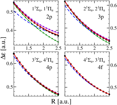
Figure 1: (Color online) Excitation energies $\Delta\epsilon$ of the H₂  molecule for the four energetically lowest dipole-allowed final states ($n=1,\ldots,4$) for different internuclear distances $R$ calculated by Staszewska and Wolniewicz Staszewska and Wolniewicz (2002); Wolniewicz and Staszewska (2003a): green triangles, $n\,^{1}\Sigma_{u}$ states; violet squares, $n\,^{1}\Pi_{u}$ states; black circles, orientationally-averaged ${}^{1}\Sigma_{u}$ and ${}^{1}\Pi_{u}$ (see text). Present excitation energies for corresponding transitions, i.e., from the ground state to 2$p$, 3$p$, 4$p$, and 4$f$: red solid curve, model potential; blue dashed curve, hydrogen atom with scaled nuclear charge H_scal.

In Fig. 1 excitation energies (EE) for the energetically-lowest dipole-allowed final states of the H₂  molecule with the symmetries $n\,^{1}\Sigma_{u}$ and $n\,^{1}\Pi_{u}$ with $n=1,\ldots,4$ are given in the range of internuclear distances $1{\rm\,a.\,u.}\leq R\leq 2.5$ a. u.  They were obtained from the very accurate calculations by Staszewska and Wolniewicz Wolniewicz (1993); Staszewska and Wolniewicz (2002); Wolniewicz and Staszewska (2003a). The orientationally-averaged molecular EE are given as circles. The corresponding four EE for an atomic system are the energy differences $\Delta\epsilon$ between the ground state and the 2$p$, 3$p$, 4$p$, and 4$f$ state.

It can be seen that in all of the four cases the EE of the model potential approximates the orientationally-averaged EE of the H₂  molecule very well in the whole $R$ range considered here. Only for the transition into the 2$p$ state the EE obtained with model potential are slightly higher than those for H₂ for large $R$. It is known that in the $R$ range which is considered here the $4\,^{1}\Sigma_{u}$ and $3\,^{1}\Pi_{u}$ states possess a dominant ($1s4f$) contribution Wolniewicz and Staszewska (2003b); Spielfiedel (2003). Consequently, these states cannot be compared to a $p$ state of the model potential but instead to the $4f$ state.

In contrast to the findings for $V_{\rm mod}$ the results for the scaled hydrogen atom H_scal differ from the other $\Delta\epsilon$ curves especially for small $R$ while they come close to the correct values for $R>2$ a. u.  For large $R$ this trend could have been expected since the H₂ molecule becomes more and more like two distant H atoms and therefore can be modeled by the hydrogen atom-like H_scal. However, it is known that, e.g., the excitation probability can depend considerably on the EE Lühr and Saenz (2008b) and therefore should be described accurately, especially around the equilibrium distance $R\approx 1.4$ a. u.

III.2 Electronic transition matrix elements

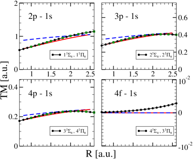
Figure 2: (Color online) Electronic transition moments (TM) of the H₂  molecule as a function of $R$ for transitions from the ground state $1^{1}\Sigma_{g}$ to the four orientationally-averaged, energetically-lowest, dipole-allowed final states consisting of the symmetries ${}^{1}\Sigma_{u}$ and ${}^{1}\Pi_{u}$: black circles, Wolniewicz and Staszewska Wolniewicz and Staszewska (2003b, a); green squares, Drira Drira (1999). Present results for corresponding transition moments, i.e., from the ground state to 2$p$, 3$p$, 4$p$, and 4$f$: red solid curve, model potential $V_{\rm mod}$; blue dashed curve, hydrogen atom with scaled nuclear charge H_scal. (Note the different scales, especially for the $4f-1s$ transition.)

Another test of the capability of the model potential $V_{\rm mod}$ given in Eq. (1) can be performed by considering transition moments (TM) which are known to be much more sensitive to the behavior of the wave functions than the energies. The dipole TM into the state $|\,nl\,\rangle$ for a fixed $R$,

$$M(nl)=\sqrt{2}\;\langle\,1s\,|\,\hat{\rm x}\,|\,nl\,\rangle\,,$$ (6)

were computed for the same transitions which have been already discussed in III.1, where $n$ and $l$ are the principal and angular momentum quantum numbers, respectively. The factor $\sqrt{2}$ in Eq. (6) accounts for the two electrons in the H₂ molecule. TM from the H₂ ground state $1\,^{1}\Sigma_{g}$ to the dipole-allowed final states ${}^{1}\Sigma_{u}$ and ${}^{1}\Pi_{u}$ were calculated by Wolniewicz and Staszewska Wolniewicz and Staszewska (2003b, a), Spielfiedel Spielfiedel (2003), and Drira Drira (1999). In Fig. 2 the orientationally-averaged molecular TM are compared to the present results obtained with the model potential, whereas the wrong assignment done in Drira (1999) for molecular states with dominant ($1s4p$) or ($1s4f$) configuration is corrected as proposed in Wolniewicz and Staszewska (2003b, a); Spielfiedel (2003). Also given are the TM for the scaled hydrogen atom H_scal.

In general, the present TM achieved with $V_{\rm mod}$ agree with the data for the full H₂ molecule. For $R>1.5$ a. u. there is some deviation for the transition into the 2$p$ state which could have been expected, since the electron-electron interaction and the effects due to the two nuclei are most prominent for the lowest excited states. Otherwise, all TM to higher states match the literature data very well. It may be noted that even the molecular states $4\,^{1}\Sigma_{u}$ and $3\,^{1}\Pi_{u}$ — both with dominant ($1s4f$) character at small $R$ — are again nicely represented by the non-dipole-allowed $4f$ state of the model. The EE as well as the vanishing TM of the $4f$ state match the corresponding orientationally-averaged results of the H₂ molecule.

The TM calculated for H_scal show for all $p$ transitions a different dependence on $R$ than the TM for H₂. For small $R$ they are too large and for $R\rightarrow 2.5$ a. u. they approach the TM calculated for $V_{\rm mod}$. The deviations indicate that, especially at small $R$, the properties of the wave functions obtained with $V_{\rm scal}$ differ considerably from those of a real H₂ molecule.

III.3 Oscillator strengths

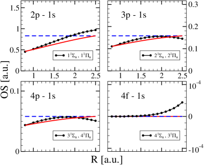
Figure 3: (Color online) Oscillator strengths (OS) of the H₂ molecule as a function of $R$ for transitions from the ground state $1^{1}\Sigma_{g}$ to the four orientationally-averaged, energetically-lowest, dipole-allowed final states consisting of the symmetries ${}^{1}\Sigma_{u}$ and ${}^{1}\Pi_{u}$: black circles, Wolniewicz and Staszewska Staszewska and Wolniewicz (2002); Wolniewicz and Staszewska (2003b, a). Results for corresponding transition moments, i.e., from the ground state to 2$p$, 3$p$, 4$p$, and 4$f$: red solid curve, present; blue dashed curve, hydrogen atom with scaled nuclear charge H_scal.

Fig. 3 shows the oscillator strengths (OS) of the H₂  molecule, the model potential $V_{\rm mod}$, and H_scal as a function of $R$ for the same transitions which were already considered before. It may be argued that the procedure of orientational averaging is most appropriate for the OS since they obey the Thomas-Reiche-Kuhn sum rule. Since the OS depend on the EE and TM the question is whether this leads to a compensation or even to an increase of the deviations between model and real molecule. The OS from the ground into the excited state $|\,nl\,\rangle$ are given by

$$f(nl)=\frac{2}{3}\,(\epsilon_{nl}-\epsilon_{0})\,|\,M(nl)\,|^{\,2}\,,$$ (7)

where $\epsilon_{0}$ and $\epsilon_{nl}$ are the energies of the ground and final excited state $|\,nl\,\rangle$, respectively. The OS for the H₂ molecule are constructed in the same way using the data calculated by Wolniewicz and Staszewska Staszewska and Wolniewicz (2002); Wolniewicz and Staszewska (2003b, a). First, the OS for both symmetries ${}^{1}\Sigma_{u}$ and ${}^{1}\Pi_{u}$ were determined separately and afterwards orientationally weighted with factors 1/3 and 2/3, respectively, in order to compare to the present results.

It can be seen in Fig. 3 that the OS of H_scal are independent of $R$ and are therefore the same as for the hydrogen atom. This is due to a cancellation of the $Z_{\rm scal}$ dependence in Eq. (7). Therein the dependence on $Z_{\rm scal}$ of the energies is $\epsilon\propto(Z_{\rm scal})^{2}$ (cf. Eq. (5)) and of the TM is $M\propto 1/(Z_{\rm scal})$. It is even necessary that the OS of H_scal are independent of $R$ since a scaling of the OS with a single factor would lead to a violation of the above mentioned sum rule.

The OS of the H₂ molecule and for $V_{\rm mod}$ are, however, not independent of the internuclear distance $R$. For all transitions the OS of H₂ and the present model agree well for small $R$. For increasing $R$ the OS obtained with $V_{\rm mod}$ increase roughly linearly while those for H₂ show a different behavior for $R>1.5$ a. u.  However, the magnitudes are still comparable. At $R=2.5$ a. u. the OS obtained with $V_{\rm mod}$ and $V_{\rm scal}$ coincide which already could have been expected before from the results for the related EE and TM. For this distance both potentials become hydrogen-atom like. Considering the region around $R=1.4$ a. u. — which is most important for many calculations with fixed $R$ considering processes starting from the H₂ ground state — one can conclude that the OS of the H₂ molecule are satisfyingly modeled by the proposed potential $V_{\rm mod}$.

III.4 Photoionization cross sections

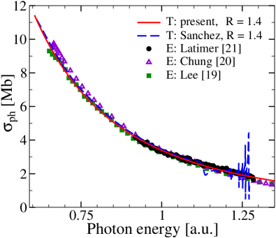
Figure 4: (Color online) Total photoionization cross section of H₂ as a function of the photon energy for a fixed internuclear distance $R=1.4$ a. u.  Theory: red solid curve, present results with model potential; blue dashed curve, Sánchez and Martín Sánchez and Martín (1997). Experiment: green squares, Lee et al. Lee et al. (1976); violet triangles, Chung et al. Chung et al. (1993); black circles, Latimer et al. Latimer et al. (1995).

A calculation of the photoionization spectrum for the hydrogen molecule is used to demonstrate the applicability of the present model to interaction processes in which an H₂ molecule is ionized. In doing so, the representation of the continuum states is probed. Further applications of $V_{\rm mod}$ in order to describe ionization of H₂ in time-dependent processes can be found elsewhere Lühr and Saenz (2008a); Vanne and Saenz (2008). The photoionization cross section is given by

$$\sigma_{\rm ph}(\epsilon)=\frac{4\,\pi^{2}}{c}\,(\epsilon-\epsilon_{0})\,\left|\,M(\epsilon)\,\right|^{\,2}\,\rho(\epsilon)\,,$$ (8)

where $\epsilon$ is the positive energy of the ionized final state $|\,\epsilon\,\rangle$ with an angular momentum $l=1$ and $c$ is the speed of light. The transition matrix elements $M(\epsilon)$ are defined in the same way as in Eq. (6) except that the $|\,\epsilon\,\rangle$ are considered as final states. The density of continuum states $\rho(\epsilon)$ is used for energy-normalization of the cross section.

The present photoionization cross sections were calculated for $R=1.4$ a. u. in order to compare the results with theoretical calculations from literature in which the fixed-nuclei approximation was used. Besides the theoretical results by Sánchez and Martín Sánchez and Martín (1997) also experimental photoionization cross sections are shown in Fig. 4 which were measured by Lee et al. Lee et al. (1976), Chung et al. Chung et al. (1993) and Latimer et al. Latimer et al. (1995).

It can be seen that the experimental photoionization cross sections are well described by the present model. At low energies, however, the results by Chung et al. and Lee et al. lie slightly above and below the present curve, respectively. The measurements by Latimer et al. where performed between approximately 0.9 and 1.3 a. u. on a dense energy grid searching for resonances above 1.1 a. u. which they did not find. Their data match very well with the present curve which is, of course, free of any resonance caused by doubly-excited states. The clearly visible resonances in the theoretical data calculated by Sánchez and Martín around $R=1.12$ and 1.25 a. u. were explained by Martín in Martín (1999) as being only visible within the fixed-nuclei approximation. In a further calculation which includes nuclear motion Martín (1999) the resonance effects are, in accordance with experimental results, practically invisible. This was explained by the broadening of the resonances, if the nuclear degrees of freedom are included. For energies below 1.1  a. u. where no resonances occur in the data of Sánchez and Martín (1997) their calculation agrees well with the present curve.

III.5 Collisional excitation cross sections

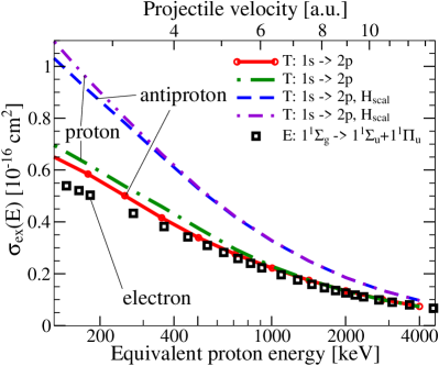
Figure 5: (Color online) Differential cross sections $\sigma_{\rm ex}$ for excitation into the lowest dipole-allowed states of H₂ as a function of the projectile velocity $v$ in  a. u. and of the equivalent proton energy $E$ in keV. Theory: Present results for a fixed internuclear distance $R=1.4$ a. u. for excitation into 2$p$. Model potential $V_{\rm mod}$: red solid curve, antiprotons; green dash-dotted curve, protons. H_scal: blue dashed curve, antiprotons; violet dash-double-dotted curve, protons. Experiment: Sum of cross sections for excitations into $1^{1}\Sigma_{u}$ and $1^{1}\Pi_{u}$: black squares, electrons, Liu et al. Liu et al. (1998).

While the ionization probability depends strongly on the ionization potential the excitation process is more sensitive to bound-state properties. Therefore, a calculation of an excitation cross section for the H₂ molecule is used to demonstrate that the model potential is also capable to describe transitions to bound states properly.

In Fig. 5 the partial cross section for the energetically-lowest, dipole-allowed transition for H₂ collisions with protons and antiprotons is shown where the H₂ target is described with the model potential. Detailed information concerning the employed time-dependent method is given elsewhere Lühr and Saenz (2008a). This transition has been chosen since first, it is the most probable excitation in this energy range and second, in Sec. III.2 and III.3 the largest deviation of the TM and OS between the model and the H₂ molecule have been observed for this transition. Furthermore, partial cross sections can be used for a more sensitive testing because the errors of total cross sections may be reduced by some error compensation. The present results are compared with experimental data for H₂  collisions with electrons measured at a temperature of 10 K by Liu et al. Liu et al. (1998) due to the fact that to the best of the authors’ knowledge no measurements have been performed for proton or antiproton impact. In addition, also results for proton and antiproton collisions with H_scal are given in Fig. 5.

The results for protons and antiprotons obtained with the proposed model potential $V_{\rm mod}$ coincide for large impact energies $E>1000$ keV as is expected. At these high energies they also fully agree with the experimental data for electrons with the same impact velocity $v$. This behavior at high impact velocities is predicted by the first Born approximation, i.e., the same cross section can be expected for collisions including particles with the same absolute value of the charge and the same impact velocity. At smaller energies the cross sections start to depend on the properties of the projectile. Thereby, the antiproton results are closer to the measured electron data than the results for proton impact since the former both share the same charge Knudsen and Reading (1992).

The H_scal results for protons and antiprotons also coincide for high impact energies as expected in the first Born limit. However, the excitation cross sections for H_scal in Fig. 5 as well as in Lühr and Saenz (2008a) clearly show a different behavior than the experimental data and the results obtained with the potential $V_{\rm mod}$.

In contrast to the present results, the use of H_scal as a target model in calculations of total ionization cross sections of an H₂ molecule can yield to a certain extent reasonable results Lühr and Saenz (2008a). The mixed capability of H_scal in describing the H₂ molecule may be explained in the following way. On the one hand, concerning ionization, the ionization potential is in both models, i.e., $V_{\rm mod}$ and $V_{\rm scal}$, by definition correct. On the other hand, the potentials differ in their $r$ dependence and the short-range as well as the long-range behavior of $V_{\rm scal}$ obviously disagrees with that of an H₂ molecule. This leads to a poor description of the bound states and finally to wrong excitation cross sections. This is in accordance with the deviations of the OS in Fig. 3 which indicate too large excitation probability for H_scal at $R=1.4$ a. u.

III.6 Helium atom

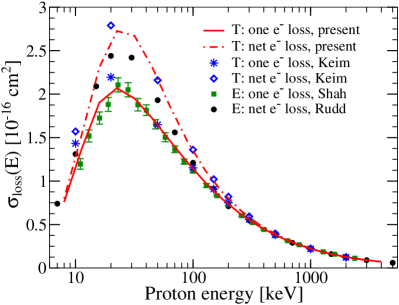
Figure 6: (Color online) Electron loss cross section of He collisions with protons. One-electron loss. Theory: red solid curve, $V_{\rm mod}$ with $\alpha=0.8791$; blue stars, Keim et al. M. Keim, A. Achenbach, H.J. Lüdde and T. Kirchner (2005). Experiment: green squares, Shah and Gilbody Shah and Gilbody (1985); Shah et al. (1989). Net electron loss. Theory: red dash–dotted curve, $V_{\rm mod}$ with $\alpha=0.8791$; blue diamonds, Keim et al. M. Keim, A. Achenbach, H.J. Lüdde and T. Kirchner (2005). Experiment: black circles, Rudd et al. Rudd et al. (1983).

In the limit $R\rightarrow 0$ with $\alpha=0.8791$ the model potential $V_{\rm mod}$ can be used for the description of a helium atom. Obviously, various different one-electron potentials have already been proposed in order to describe He atoms. There are, e.g., the well-known Thomas-Fermi and Hartree models as well as the Hartree-Fock-Slater (HFS) model Slater (1951) which includes a local exchange correction and was applied, e.g., in Gulyás et al. (1995). Another approach is the optimized potential method (OPM) discussed in Kirchner et al. (1997); K. Aashamar (1978) which was used to calculated $p$ + He loss cross sections in M. Keim, A. Achenbach, H.J. Lüdde and T. Kirchner (2005).

In Fig. 6 electron loss cross sections (the sum of ionization and capture) are shown for collisions of protons with He atoms. The present results were obtained with the same method which was employed for the $p$ and $\bar{p}$ collisions with H₂ in section III.5 and which was discussed in detail in Lühr and Saenz (2008b, a). Measurements of the one-electron loss were performed by Shah and Gilbody Shah and Gilbody (1985); Shah et al. (1989). Cross sections for the net electron loss were experimentally determined by Rudd et al. Rudd et al. (1983). Calculations of the one-electron and net electron loss were done by Keim et al. M. Keim, A. Achenbach, H.J. Lüdde and T. Kirchner (2005) using the OPM with a time-independent effective potential.

In the present results for the net electron loss the probabilities for double capture, double ionization, and transfer ionization are counted twice in order to get the correct number of electrons lost in the collision process. All theoretical data points for the net electron loss by Keim et al. coincide fully with the present findings apart from those for the two lowest impact energies (10 and 20 keV) which are clearly higher than the present ones. The present net loss cross sections reproduce the experimental data by Rudd et al. to a great extent. However, in the energy range $20<E<100$ keV the experimental data are smaller than the outcome of both theoretical investigations.

In the case of the one-electron loss the present findings match the experimental results by Shah and Gilbody well in the whole impact energy range of the protons. Again all theoretical data points by Keim et al. coincide fully with the present ones besides those for the two lowest impact energies which have again larger values. Finally, it can be concluded that in addition to H₂ the proposed model potential $V_{\rm mpd}$ is also capable of a simple description of He atoms which is consistent with the OPM without response.

IV Conclusion

A simple model potential $V_{\rm mod}$ for an effective one-electron, single-centered description of the H₂ molecule has been proposed and its properties have been examined. The potential is unambiguously determined by the correct ionization potential of the H₂ molecule and allows for the description of H₂ at an arbitrary internuclear distance $R$. Thereby, also the nuclear motion can be considered to a some extent.

The model potential was used for various applications in the range $0.8\leq R\leq 2.5$ a. u.  The energetically-lowest, dipole-allowed excitation energies, transition moments as well as oscillator strengths of the H₂ molecule are represented well by the present model. The model was furthermore employed for the calculation of the photoionization cross section of H₂ and a partial excitation cross section in collisions of H₂ with charged particles. In both applications experimental and also theoretical literature data could be well described by the present results obtained with the model potential.

Concerning the scaled hydrogen atom as model for H₂ the results for ionization are satisfying while bound states properties and therefore also excitation cross sections are not reproduced adequately.

The satisfying description of results for H₂ molecules justifies on the one hand the choice of the ionization potential of H₂ as a criterion for adjusting $V_{\rm mod}$ to a certain internuclear distance. On the other hand, together with the surpassing simplicity of the model which includes an approximate analytic expression for the ionization potential, it suggests its applicability to a large number of further problems. To name only some, there are, e.g., the description of the electronic structure of H₂ molecules in H₂ clusters, H₂ molecules interacting with external fields or with particles, and finally also the modeling of He atoms in the limit $R\rightarrow 0$.

It can be concluded that the H₂ molecule is in many cases surprisingly well described by a single-electron, one-center model. This means, that in these cases the effects of charge anisotropy and two-electron effects are small.

ACKNOWLEDGMENTS

The authors wish to thank H. J. Lüdde for a discussion on effective one-electron models. The authors also would like to thank F. Martín and T. Kirchner for providing cross sections in numerical form. The authors are grateful to BMBF (FLAIR Horizon), DFG, and Stifterverband für die deutsche Wissenschaft for financial support.

References

- Vanne and Saenz (2008) Y. V. Vanne and A. Saenz, J. Mod. Opt. 55, 2665 (2008).
- Lühr and Saenz (2008a) A. Lühr and A. Saenz, Phys. Rev. A 78, 032708 (2008a).
- Teller and Sahlin (1970) E. Teller and H. L. Sahlin, in Physical chemistry. An advanced tratise. 5. Valency, edited by H. Eyring (Academic Press, New York, 1970), section 2.C.
- Hartree (1957) D. R. Hartree, The Calculation of Atomic Structures (Wiley, New York, 1957), section 2.5.
- Wolniewicz (1993) L. Wolniewicz, J. Chem. Phys. 99, 1851 (1993).
- NIST (2008) (National Institue of Standards and Technology) NIST (National Institue of Standards and Technology), http://physics.nist.gov/PhysRefData/ASD/index.html (2008).
- Saenz and Froelich (1997) A. Saenz and P. Froelich, Phys. Rev. C 56, 2162 (1997).
- Errea et al. (1997) L. F. Errea, J. D. Gorfinkiel, A. Macías, L. Méndez, and A. Riera, J. Phys. B: At. Mol. Phys. 30, 3855 (1997).
- Ermolaev (1993) A. M. Ermolaev, Hyperfine Interact. 76, 335 (1993).
- Wang et al. (1995) Y. D. Wang, C. D. Lin, N. Toshima, and Z. Chen, Phys. Rev. A 52, 2852 (1995).
- Apalategui and Saenz (2002) A. Apalategui and A. Saenz, J. Phys. B: At. Mol. Phys. 35, 1909 (2002).
- Staszewska and Wolniewicz (2002) G. Staszewska and L. Wolniewicz, J. Mol. Spectrosc. 212, 208 (2002).
- Wolniewicz and Staszewska (2003a) L. Wolniewicz and G. Staszewska, J. Mol. Spectrosc. 220, 45 (2003a).
- Wolniewicz and Staszewska (2003b) L. Wolniewicz and G. Staszewska, J. Mol. Spectrosc. 217, 181 (2003b).
- Spielfiedel (2003) A. Spielfiedel, J. Mol. Spectrosc. 217, 162 (2003).
- Lühr and Saenz (2008b) A. Lühr and A. Saenz, Phys. Rev. A 77, 052713 (2008b).
- Drira (1999) I. Drira, J. Mol. Spectrosc. 198, 52 (1999).
- Sánchez and Martín (1997) I. Sánchez and F. Martín, J. Phys. B: At. Mol. Phys. 30, 679 (1997).
- Lee et al. (1976) L. C. Lee, R. W. Carlson, and D. L. Judge, J. Quant. Spectrosc. Radiat. Transfer 16, 873 (1976).
- Chung et al. (1993) Y. M. Chung, E.-M. Lee, T. Masuoka, and J. A. R. Samson, J. Chem. Phys. 99, 885 (1993).
- Latimer et al. (1995) C. J. Latimer, K. F. Dunn, F. P. O’Neill, M. A. MacDonald, and N. Kouchi, J. Chem. Phys. 102, 722 (1995).
- Martín (1999) F. Martín, J. Phys. B: At. Mol. Phys. 32, R197 (1999).
- Liu et al. (1998) X. Liu, D. E. Shemansky, S. M. Ahmed, G. K. James, and J. M. Ajello, J. Geophys. Res. A 103, 26739 (1998).
- Knudsen and Reading (1992) H. Knudsen and J. F. Reading, Phys. Rep. 212, 107 (1992).
- M. Keim, A. Achenbach, H.J. Lüdde and T. Kirchner (2005) M. Keim, A. Achenbach, H.J. Lüdde and T. Kirchner, Nucl. Instr. Meth. Phys. Res. B 233, 240 (2005). M. Keim, Ph.D. thesis, Universität Frankfurt, Germany (2005).
- Shah and Gilbody (1985) M. B. Shah and H. B. Gilbody, J. Phys. B: At. Mol. Phys. 18, 899 (1985).
- Shah et al. (1989) M. B. Shah, P. McCallion, and H. B. Gilbody, J. Phys. B: At. Mol. Phys. 22, 3037 (1989).
- Rudd et al. (1983) M. E. Rudd, R. D. DuBois, L. H. Toburen, C. A. Ratcliffe, and T. V. Goffe, Phys. Rev. A 28, 3244 (1983).
- Slater (1951) J. C. Slater, Phys. Rev. 81, 385 (1951).
- Gulyás et al. (1995) L. Gulyás, P. D. Fainstein, and A. Salin, J. Phys. B: At. Mol. Phys. 28, 245 (1995).
- Kirchner et al. (1997) T. Kirchner, L. Gulyás, H. J. Lüdde, A. Henne, E. Engel, and R. M. Dreizler, Phys. Rev. Lett. 79, 1658 (1997).
- K. Aashamar (1978) J. D. T. K. Aashamar, T. M. Luke, Atomic Data and Nuclear Data Tables 22, 443 (1978).