Noise in random Boolean networks

Abstract

We investigate the effect of noise on Random Boolean Networks. Noise is implemented as a probability $p$ that a node does not obey its deterministic update rule. We define two order parameters, the long-time average of the Hamming distance between a network with and without noise, and the average frozenness, which is a measure of the extent to which a node prefers one of the two Boolean states. We evaluate both order parameters as function of the noise strength, finding a smooth transition from deterministic ($p=0$) to fully stochastic ($p=1/2$) dynamics for networks with $K\leq 2$, and a first order transition at $p=0$ for $K>2$. Most of the results obtained by computer simulation are also derived analytically. The average Hamming distance can be evaluated using the annealed approximation. In order to obtain the distribution of frozenness as function of the noise strength, more sophisticated self-consistent calculations had to be performed. This distribution is a collection of delta peaks for $K=1$, and it has a fractal sructure for $K>1$, approaching a continuous distribution in the limit $K\gg 1$.

I Introduction

Random Boolean Networks (RBNs) Kauffman (1969); Drossel (2008) have been used as a simple model for a variety of dynamical systems consisting of interacting units, such as neural networks Rosen-Zvi et al. (2001), social networks Moreira et al. (2004) and, more prominently, gene regulatory networks Lagomarsino et al. (2005); Kauffman (1969). RBNs are composed of Boolean nodes that are coupled to each other. In the case of gene regulatory networks, the Boolean state is a step-function approach to the expression level of a particular gene. Despite this loss of detail, the most important features of gene regulatory processes are still captured in many cases, since they should not depend on biochemical details, but on the desired sequence of events in the cell Bornholdt (2005).

So far, the dynamics of RBNs have mostly been studied using deterministic update rules. The dynamics of such models are non-ergodic, with periodic attractor trajectories in state space. Once the system has reached an attractor, it remains there. Another important property of RBNs is a phase transition, which occurs when the number $K$ of inputs per node is changed. For unbiased networks, the dynamics exhibit a frozen phase at $K=1$, where local perturbations die out quickly and most attractors are fixed points, and a “chaotic” phase at $K>2$, where perturbations increase exponentially fast and attractors have very long periods. At the boundary $K=2$ between those two phases are the so-called “critical” networks, where perturbations increase algebraically with time. Originally, it was suggested by Kauffmann Kauffman (1969) that such critical networks are best suited to model real systems, which are supposedly poised “at the edge of chaos”. In the meantime, there is agreement that RBNs of all three types have only limited validity when applied to real systems.

Real networks usually have some level of stochastic behaviour, and for this reason several authors have investigated RBNs under the influence of stochasticity. For instance, in Greil and Drossel (2005) the nodes of RBNs were updated in a completely random order. This update method preserves the non-ergodicity of the system, and it is still possible to identify distinct attractors. Attractors are in this case defined as sets of states all of which are visited for a non-vanishing proportion of time during the same trajectory. The stochastic update sequence vastly reduces the number of attractors of critical RBNs, which becomes a power law as function of the network size. Similar results are obtained when the update sequence deviates only slightly from a synchronous update Klemm and Bornholdt (2005). Such a power law was for a long time falsely believed to occur in deterministic RBNs  Kauffman (1969); Samuelsson and Troein (2003); Drossel (2005); Drossel et al. (2005).

Instead of introducing stochasticity into the update times, other authors introduce it into the update functions. In Shmulevich et al. (2002), probabilistic Boolean functions are used, where a set of several Boolean functions is assigned to each node, and at each time step one of these is chosen randomly with a given probability. According to Shmulevich et al. (2002), this model is more realistic than models with a purely deterministic update scheme.

However, the most important way of introducing noise into a RBN is in form of a “temperature”, leading often to ergodic behavior. The effect of thermal noise on Ising spins on a network was studied in Indekeu (2004); Aleksiejuk et al. (2002), where a “ferromagnetic” transition from the ordered to the disordered phases was observed at a critical noise strength value. In the language of gene regulatory networks, a temperature manifests itself as fluctuations in the protein concentrations, so that a gene may not always be turned on or off, given the same expression state of the other genes McAdams and Arkin (1997). This effect can be included into models by allowing a deviation from the deterministic update rule with a certain probability. In Fretter and Drossel (2008), for instance, a subset of nodes were perturbed in this way (this corresponds to turning on the temperature for a short time interval), and the response of the dynamics to this perturbation was evaluated, giving information about the basin structure of the system. Miranda et al. Miranda and Parga (1989) studied the effect of a permanently acting temperature by introducing a fixed probability $p$ that the state of a node becomes the opposite of what it should be according to the deterministic update rule. They evaluated the average crossing time between trajectories in state space which started from different initial states as function of noise strength Miranda and Parga (1989); Golinelli and Derrida (1989); Qu et al. (2002). By sampling the entire state space of small networks ($N\leq 20$), it was found that the “barriers”, which correspond to the attractor basin boundaries, can be crossed with non-vanishing probability when $p>0$, although the characteristic times may be large. This means that the system is always ergodic. This type of noise has also been studied for Boolean networks with threshold functions, corresponding to a majority update rule Huepe and Aldana-González (2002). This system undergoes a second order phase transition at a critical noise strength from an ordered dynamical phase, where all nodes assume the same value for the majority of time, to a disordered phase where nodes assume both states equally often.

In this work, we investigate the effect of ongoing stochastic noise on RBNs. Following Miranda and Parga (1989); Golinelli and Derrida (1989); Qu et al. (2002), noise strength is tuned via a probability $p$ that a node does not obey its deterministic update rule. We monitor the transition from fully deterministic dynamics ($p=0$) to purely stochastic dynamics ($p=1/2$) as the noise strength is varied. Differently from Miranda and Parga (1989); Golinelli and Derrida (1989); Qu et al. (2002), we are interested in the behaviour of the networks in the limit of large system size, where it is impossible to explore large parts of the state space. In order to characterize the transition from zero to infinite temperature, we define two order parameters: the long-time average of the Hamming distance between a network with and without noise, and the average frozenness, which is a measure of the extent to which a node prefers one of the two Boolean states. We find, both analytically and numerically, that this transition for the Hamming distance is continuous for $K\leq 2$, and discontinuous at $p=0$ for $K>2$, when the Hamming distance is considered. This distinction is a direct consequence of the phase transition from frozen to chaotic dynamics in the deterministic model. The frozenness shows a smooth transition for all values of $K$. The distribution of frozenness shows a surprising richness in structure, as revealed by computer simulations. For $K\leq 2$ and for $K\gg 1$, we succeeded in reproducing this structure as function of $p$ by analytical considerations.

The remainder of this paper is divided into the following parts: In Sec. II we define the RBN model and the type of noise used for our study. In Sec. III, we define the first order parameter, the Hamming distance, and evaluate it numerically and analytically. In Sec. IV, we define the second order parameter, the frozenness, and evaluate it using computer simulations and analytical considerations. Finally, we summarize and discuss our findings in Sec. V.

II Model

A Boolean network is defined as a directed network of $N$ nodes representing Boolean variables $\bm{\sigma}\in\{1,0\}^{N}$, which are subject to a dynamical update rule,

$$\bm{\sigma}(t+1)=\bm{f}\left(\bm{\sigma}(t)\right),$$ (1)

where $f_{i}$ is a function assigned to node $i$ that depends exclusively on the states of its inputs.

We introduce noise into the system through a probability $p$ that a node does not obey its deterministic update rule,

$$\bm{\sigma}(t+1)=\bm{f}\left(\bm{\sigma}(t)\right)\veebar\bm{n},$$ (2)

where $\bm{n}$ is a random vector, with elements $n_{i}$ being $1$ with probability $p$ and $0$ otherwise. The symbol $\veebar$ represents the “exclusive or” Boolean operation. Hence, for $p=0$ the deterministic behaviour is recovered, and for $p=1/2$ the dynamics is completely stochastic.

RBNs are a special case of Boolean networks, where all possible Boolean functions are assigned randomly to each node with the same probability, and where the nodes are randomly connected. The number of inputs of each node is fixed at a value $K$. The random wiring leads to a Poisson distribution with mean $K$ for the number of outputs. When updated deterministically, RBNs are in the frozen phase for $K=1$. After a transient time, they reach an attractor where all nodes (or all nodes apart from a small number) are permanently frozen in one of the two Boolean states. Networks with larger $K$ have also a frozen core of nodes for $p=0$, and the nodes belonging to it become frozen after a transient time. For $K=2$, all but of the order of $N^{2/3}$ nodes belong to the frozen core. With increasing $K$, the frozen core contains an ever smaller proportion of nodes. For $K=2$, the nonfrozen part of the network consists of several independent components. Each of these components contains a set of relevant nodes, which are connected such that there is at least one feedback loop among them, and “trees” of nonfrozen nodes which are rooted in the relevant nodes and which are slaved to the dynamics of the relevant nodes.

III Average Hamming distance

III.1 Definition

We use the average in time of the Hamming distance between the states of two copies of a network in order to quantify the effect of noise on the dynamics. Consider a given network in the initial state $\bm{\sigma}(t=0)$, and an exact replica, which is initially in the same state, $\bm{\sigma}^{\prime}(t=0)=\bm{\sigma}(t=0)$. The dynamics of both networks are evolved in parallel, but noise is applied only to $\bm{\sigma}^{\prime}(t)$, as in Eq. (2). The mean Hamming distance $h(t)$ between the two networks is defined as

$$h(t)=\frac{1}{N}\langle\left|\sigma_{i}(t)-\sigma_{i}^{\prime}(t)\right|\rangle\,,$$ (3)

where $\langle\dots\rangle$ denotes the average over the noise.

The long-time average $h$ of the Hamming distance is defined as

$$h=\lim_{T\to\infty}\frac{1}{T}\frac{1}{N}\sum_{t,i}\left|\sigma_{i}(t)-\sigma_{i}^{\prime}(t)\right|.$$ (4)

If the trajectories become completely uncorrelated after some time, we have $h=1/2$. If the trajectories remain closer in state space, we have $h<1/2$. The case $h>1/2$ does not occur in our model and is therefore not considered in this paper.

III.2 Annealed approximation

We will first evaluate analytically the Hamming distance by using the so-called annealed approximation Derrida and Pomeau (1986). This is a mean field theory, which neglects correlations between nodes and the finite size of the network. The annealed approximation corresponds to the behaviour of a (infinitely large) network where all the edges are randomly rewired at each time step. Within the annealed approximation, the dynamics of a RBN without noise (i.e. for $p=0$) is fully specified by the parameter $\lambda$, which is $K$ times the probability that a node changes its state when one (or more) of its inputs is flipped. For RBNs, we have $\lambda=K/2$, since for any input combination, there is an equal probability that the output of a function will be either $0$ or $1$. When considering two replicas of a network, $\lambda$ is identical to the mean number of nodes that assume a different state in the two networks at time $t=1$ when at time $t=0$ the state of only one node was different.

At any time, the Hamming distance between a network with noise and its twin noiseless counterpart, as described by Eq. (3), is simply the fraction of nodes which were changed by noise or by the effect of previously changed nodes. The time evolution of $h(t)$ can then be described as the evolution of the population of flipped nodes. (A node in the replica with noise is called “flipped” it its state deviates from the state it has in the replica without noise.) Let $q(h(t))=1-(1-h(t))^{K}$ denote the probability that a node has at least one flipped input. Then the probability $h(t+1)$ that a node is flipped at time $t+1$ can be written as

$$\begin{split}h(t+1)&=\frac{\lambda}{K}q(1-p)+\left(1-\frac{\lambda}{K}\right)pq+(1-q)p\\ &=\frac{\lambda(1-2p)}{K}\left[1-\left(1-h(t)\right)^{K}\right]+p,\\ \end{split}$$ (5)

where the first term in the first line corresponds to the proportion of nodes that are flipped by previously flipped nodes (and are not flipped back by noise), and the second and third term are the proportion of nodes that are flipped by noise (with or without inputs being flipped). The fixed point of Eq. (5) determines the order parameter $h$, for given $K$ and $p$. We evaluated this fixed point numerically. Fig. 1 shows $h$ as function of the noise strength $p$ for several values of $K$. The solid lines are the fixed point solutions of Eq. (5), the symbols represent the result of computer simulations of quenched RBNs. The agreement between the annealed approximation and the real networks is very good.

The most striking feature of Fig. 1 is the existence of a first-order transition at $p=0$ for $K>2$. This is due to the phase transition to “chaotic” behaviour for $K>2$. In chaotic networks, even the smallest local perturbations have a global effect.

III.3 The Hamming distance on subsets of nodes

We next evaluate separately the Hamming distance for the frozen core and for the nonfrozen part of the network. Fig. 2 shows the long-time Hamming distance, evaluated only for the nodes that belong to the frozen core. These curves can be fitted using the annealed approximation Eq. (5) under the condition that the factor $\lambda/K$ on the right-hand side of Eq. (5) (representing the probability that a node is flipped when at least one input is flipped) is replaced with $\lambda_{\text{eff}}/K$, with $\lambda_{\text{eff}}$ being used as a fit parameter. For $K=1$ and $2$, the frozen core is virtually indistinguishable from the rest of the network, and $\lambda_{\text{eff}}=\lambda$, but for $K>2$, $\lambda_{\text{eff}}$ decreases with increasing $K$. The reason is that the frozen core becomes composed mainly of nodes with constant functions which have $\lambda_{\text{eff}}=0$.

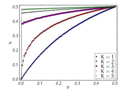
Figure 1: (Color online) Average Hamming distance as function of noise strength for RBNs of size $N=10^{4}$ for different values of $K$. Each point was obtained by averaging the results over 3 different network realizations. The solid lines are the respective steady-state solutions of Eq. (5).

Before evaluating $h$ for the nonfrozen nodes, let us consider the simplest possible connected set of nonfrozen nodes, which is a simple loop. For $K=1$ and $K=2$, such simple loops of nonfrozen nodes play an important role at determining the attractors with periods larger than 1 Kaufman and Drossel (2005), however, a considerable fraction of $K=2$ networks also have more complex relevant components. The effect of noise on such loops is very different from its effect on the frozen core, since if one of its nodes is flipped, this flip propagates indefinitely around the loop. One can calculate the accumulation of flips on such loops by considering the average Hamming distance at a given time between a loop without and with noise,

$$\begin{split}h(t)&=\sum_{i=0}^{\lfloor\frac{t-1}{2}\rfloor}{t\choose 2i+1}p^{2i+1}(1-p)^{t-(2i+1)}\\ &\approx\sum_{i=0}^{\lfloor\frac{t-1}{2}\rfloor}\frac{(tp)^{2i+1}e^{-tp}}{(2i+1)!}\\ &\approx\frac{1}{2}\left(1-e^{-2tp}\right)\,.\end{split}$$ (6)

The first equation evaluates the probability that a node has been flipped an odd number of times, and the subsequent transformations are valid for $t\gg 1$. The Hamming distance approaches the value $1/2$ with an exponential decay, and with an characteristic time $\tau=1/(2p)$.

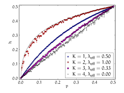
Figure 2: (Color online) Average Hamming distance as function of noise for RBN of size $N=10^{4}$ for different values of $K$. Only nodes belonging to the frozen core of the network (without noise) were considered. Each point on each curve was obtained by averaging the results for 3 different network realizations. The solid lines are the respective solutions of Eq. (5), with $\lambda_{\text{eff}}$ being used as a fit parameter.

We evaluated how fast a trajectory leaves an attractor in the presence of noise by first letting the system approach an attractor and by then turning on the noise and measuring the Hamming distance $h(l)$ to the initial state after one attractor period $l$. This is identical to the distance from the state of the noiseless replica, which returns to the initial state at time $l$. Fig. 3 shows the values of $h(l)$ for RBNs with different values of $K$. For $K=1$, the data match Eq. (6) very well, since the nonfrozen part of the network in this case can only be composed of simple loops. For $K\geq 2$, the data points are considerably above this exponential curve because a node can become flipped via many different paths. The data are better fitted using Eq. (5), in particular for long periods (i.e. large times). Just as for the case of the frozen core, $\lambda_{\text{eff}}$ was used as a fit parameter.

For smaller values of the attractor period, the data are considerably below the fitted line. The reason is that these attractor periods are much smaller than typical attractor periods, and networks with such short attractors are not characteristic of the ensemble, but have a state-space structure with a smaller set of recurrent states. Consequently trajectories diverge less fast than in typical networks.

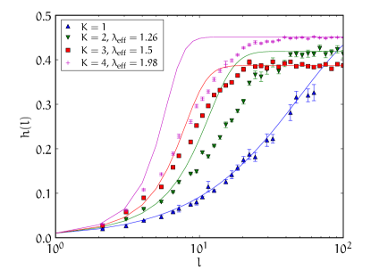
Figure 3: (Color online) Average Hamming distance $h(l)$ of the relevant components of RBNs with different values of $K$, after a full period $l$, with $p=0.01$. The curves were obtained by sampling at least $2\times 10^{4}$ attractors of several distinct RBNs of sizes $N=10^{2}$, $50$ and $25$ for $K\leq 2$, $3$ and $4$, respectively. The solid lines are given by Eq. 6 for $K>1$ and Eq. 5 for $K\geq 2$.

IV Frozenness

IV.1 Definition

The “frozenness” of a network measures the extent to which the nodes spend more time in one of the two Boolean states. It is zero, when the nodes spend the same time in both states, and it is 1 when the network is frozen. The frozenness of node $i$ is defined by the expression

$$\Omega_{i}=\left(q_{0}^{(i)}-q_{1}^{(i)}\right)^{2},$$ (7)

where $q_{\sigma}^{(i)}$ is the proportion of time node $i$ is in state $\sigma$,

$$q^{(i)}_{\sigma}=\lim_{T\to\infty}\frac{1}{T}\sum_{t=0}^{T}\delta_{\sigma_{i}(t),\sigma}.$$ (8)

By eliminating one of the two probabilities from Eq. (7), we obtain

$$\Omega_{i}=\left(2q_{\sigma}^{(i)}-1\right)^{2},$$ (9)

where $\sigma$ is either $0$ or $1$.

The frozenness $\langle\Omega\rangle$ of the network is obtained by averaging over the nodes. Figure 4 shows the frozenness $\langle\Omega\rangle$ as function of the noise strength $p$ obtained by computer simulations of networks of size $10^{4}$, for different $K$.

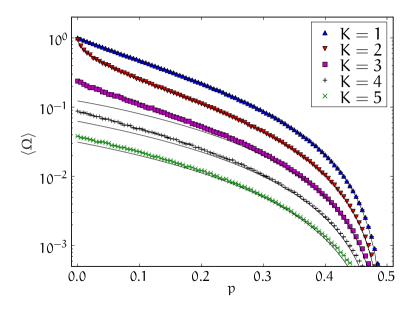
Figure 4: (Color online) Frozenness as function of noise strength for RBNs of size $N=10^{4}$ for different values of $K$. Each curve was obtained by averaging the results for 100 different network realizations. The solid lines correspond to the averages of $\rho_{\Omega}(\Omega|K,p)$, obtained in Secs. IV.2, IV.3 and IV.4, for $K=1$, $2$ and $\geq 3$, respectively.

At $p=0$, the frozenness corresponds obviously to the size of the frozen core, and it decreases towards 0 as the noise strength approaches the value 0.5.

In order to derive these curves analytically, the annealed approximation is of no use, since a network that is rewired during the course of time has very small frozenness, which is due uniquely to the constant functions. Therefore, a simple analytical calculation, which does not require the consideration of correlations between nodes, can only be performed for nodes with constant functions: for such nodes the frozenness is given by

$$\Omega_{i}=(1-2p)^{2}\,.$$ (10)

In the following, we will present more advanced analytical evaluations and further computer simulations for RBNs with different values of $K$.

IV.2 $K=1$

For $K=1$ there are only $2^{2^{1}}=4$ possible Boolean functions, two of which are constant ($1$ or $0$), and the remaining ones are the copy ($f(\sigma)=\sigma$) and invert ($f(\sigma)=\lnot\sigma$) functions. As far as the analysis of frozenness is concerned, there are only two distinct functions, constant and non-constant, since the output value is not relevant, but only how often it changes. Since each of the two types of functions occurs equally often in a $K=1$ RBN, we have $\lambda=1/2$, but $K=1$ networks with other values of $\lambda$ can also be constructed.

In a network with $K=1$, each node has only one input, and this input node also has one input, etc. In order to evaluate the probability that a node is flipped, one only needs to consider the chain of those nodes that can have an influence on the considered node. Nodes with constant functions present a barrier to the propagation of a perturbation, since they do not respond to a change in their inputs, and therefore the chain ends (or, more precisely, begins) at a node with a constant function.

Without loss of generality, we define $q^{(i)}$ as being the proportion of time node $i$ assumes its most frequent value,

$$q^{(i)}\equiv\max(q^{(i)}_{\sigma},1-q^{(i)}_{\sigma})\;\in\left[1/2,1\right].$$ (11)

Since the value of $q^{(i)}$ is fully determined by the distance of node $i$ to a node with a constant function, we choose the label $i$ in the remainder of this subsection to signify this distance. If the node itself has a constant function, we have $i=0$, if the node has a non-constant function, but its input has a constant function, we have $i=1$, etc.

The value of $q^{(0)}$, i.e. for nodes with constant functions, is simply

$$q^{(0)}(p)=1-p.$$ (12)

For larger values of $i$, we have the recursion relation

$$\begin{split}q^{(i)}&=(1-p)q^{(i-1)}+(1-q^{(i-1)})p\\ &=\frac{1}{2}(1-2p)^{i+1}+\frac{1}{2},\end{split}$$ (13)

where the solution of the recursion relation was obtained using Eq. (12). The probability of finding a given $q^{(i)}$ in the network is

$$p_{q}(q^{(i)}|p)=(1-\lambda)\lambda^{i}=\left(\frac{1}{2}\right)^{i+1}\,.$$ (14)

The frozenness of the network is thus given by

$$\left<\Omega\right>(p)=\sum_{i}p_{q}(q^{(i)}|p)(1-2q^{(i)})^{2}\,,$$ (15)

which is plotted in Figure 4 and fits the curve for $K=1$ well.

Although networks with $K=1$ have only a discrete set of possible $q$-values, the distribution of $q$ values appears as a continuum when determined by computer simulations. There are two reasons for this. First, the data points for $q$ close to 1/2 (i.e. for $\Omega$ close to 0) are so close to each other that they cannot be resolved, since a computer simulation uses a non-vanishing bin size. Solving Eq. (13) for $i$, inserting the result in (14), and using the relation $\rho_{q}(q|K=1,p)dq=p_{q}(q|K=1,p)$ with $dq=q^{(i)}-q^{(i+1)}$, we obtain

$$\rho_{q}(q|K=1,p)\propto(2q-1)^{\frac{\ln\lambda}{\ln(1-2p)}-1}\,,$$ (16)

with $\lambda=1/2$ for RBNs. Thus, in the limit $q\to 1/2$ the distribution of $2q-1$ follows as a power-law with an exponent given by the above expression. The probability density of $\Omega$ also decays as a power law, in the limit $\Omega\to 0$, but with a different exponent, since

$$\begin{split}\rho_{\Omega}(\Omega|K=1,p)=&\;\rho_{q}\left(\left.\frac{\sqrt{\Omega}+1}{2}\right|K=1,p\right)\frac{dq}{d\Omega}\\ \sim&\;\Omega^{\frac{\ln\lambda}{\ln(1-2p)}-3/2}\,.\end{split}$$ (17)

Second, a computer simulation averages only over a finite amount of time, $T$, and therefore the measured values $q^{\prime}$ are Gaussian distributed around the exact value $q$,

$$\begin{split}\tilde{\rho}_{q^{\prime}}(q^{\prime}|K=1,T,q)\approx\frac{1}{\sqrt{2\pi q/T}}e^{-\frac{(q^{\prime}-q)^{2}}{2q/T}},\end{split}$$ (18)

This dependence on $T$ can be included in Eq. (14) to obtain the probability density function for $q$

$$\begin{split}\rho_{q}(q|K=1,p,T)=&\,(1-\lambda)\sum_{i=0}^{\infty}\lambda^{i}\tilde{\rho}_{q^{\prime}}(q|T,q^{(i)}).\end{split}$$ (19)

For the distribution of $\Omega$ values, we obtain

$$\rho_{\Omega}(\Omega|K,p,T)=\rho_{q}\left(\left.\frac{\sqrt{\Omega}+1}{2}\right|K,p,T\right)\frac{1}{2\sqrt{\Omega}}.$$ (20)

Fig. 5 shows the distribution of the frozenness for a quenched network with $K=1$, for several values of $p$. It can be seen that there is very good agreement with Eq. (20). The presence of fluctuations significantly deviates some of the distributions from the expected power-law decay. For $p=0.01$, the small values of frozenness, which are not in agreement with the theoretical result, are due to the existence of loops, which are omitted in the analysis above. The probability that a node is part of a nonfrozen loop tends to zero as the network becomes larger, and therefore these points vanish in the limit of infinite system size.

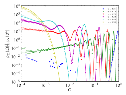
Figure 5: (Color online) Distribution of the frozenness for different values of the noise strength for RBNs of size $N=10^{5}$ for $K=1$ and $T=10^{4}$. Each curve was obtained by averaging over 100 different network realizations. The solid lines are given by Eq. (20).

IV.3 $K=2$

As $K$ becomes larger, the number of possible functions grows very fast as $2^{2^{K}}$, and a detailed analysis of the frozenness, as was done for $K=1$, becomes more complicated. The values of $q$ are still discontinuously distributed, but their number increases fast with $K$, due to the numerous combinations of Boolean functions that can determine the $q$-values of the $K$ inputs of a node and thus, in combination with the node’s Boolean function, the $q$-value of its output. Here we will lay out the basic considerations needed to obtain the distribution of $q$ for all $K>1$, and we will obtain by numerical iteration the distribution for $K=2$. Without loss of generality, we redefine $q$ as $q\equiv q_{\sigma=1}$, i.e., the fraction of time a given node has the value 1 (as opposed to Eq. (11), which simplified the case $K=1$).

In general, the probability density function $\rho_{q}(q|K=1,p)$ needs to account for all possible recursive combinations of output functions and their inputs. We can thus write the following self-consistent expression,

$$\rho_{q}(q|K,p)=\int_{0}^{1}\dotsi\int_{0}^{1}\sum_{f}p_{f}\delta(q^{(f)}-q)\prod_{i=1}^{K}\rho_{q}(q^{(i)}|K,p)dq^{(i)},$$ (21)

where the sum is taken over all Boolean functions; $p_{f}$ is the probability of the $f$th Boolean function ($p_{f}=2^{-2^{k}}$ ), and

$$q^{(f)}=(1-2p)q^{(f)}(\{q^{(i)}\})+p,$$ (22)

where $q^{(f)}(\{q^{(i)}\})$ is the value of $q$ for a specific function $f$, given the values $\{q^{(i)}\}$ of its inputs, for $i=1,\dots,K$.

Since Eq. (21) involves an expression $q^{(f)}(\{q^{(i)}\})$ for all Boolean functions, a general closed solution becomes unfeasible. However, for $K=2$ Eq. (21) can at least be solved numerically, since there are only $16$ possible functions, given in Table 1. Eq. (21) is then solved by iteration, until convergence to a self-consistent $q$ distribution is obtained. We started with the initial distribution

$$\rho^{0}_{q}(q|K,p)=\frac{1}{2}\delta(q-p)+\frac{1}{2}\delta(q-(1-p))\,.$$ (23)

In the end, we determined the final distribution $\rho_{\Omega}(\Omega|K=2,p)$ by using Eq. (20).

$f$	$f_{i}(\sigma_{1},\sigma_{2})$	$q^{(f)}(q_{1},q_{2})$
$0$	$0$	$0$
$1$	$\sigma_{1}\land\sigma_{2}$	$q_{1}q_{2}$
$2$	$\sigma_{1}\land\lnot\sigma_{2}$	$q_{1}(1-q_{2})$
$3$	$\sigma_{1}$	$q_{1}$
$4$	$\lnot\sigma_{1}\land\sigma_{2}$	$(1-q_{1})q_{2}$
$5$	$\sigma_{2}$	$q_{2}$
$6$	$\sigma_{1}\veebar\sigma_{2}$	$q_{1}+q_{2}-2q_{1}q_{2}$
$7$	$\sigma_{1}\lor\sigma_{2}$	$q_{1}+q_{2}-q_{1}q_{2}$
$8$	$\lnot(\sigma_{1}\lor\sigma_{2})$	$1-q^{(7)}(q_{1},q_{2})$
$9$	$\lnot(\sigma_{1}\veebar\sigma_{2})$	$1-q^{(6)}(q_{1},q_{2})$
$10$	$\lnot\sigma_{2}$	$1-q_{2}$
$11$	$\sigma_{1}\lor\lnot\sigma_{2}$	$q^{(7)}(q_{1},1-q_{2})$
$12$	$\lnot\sigma_{1}$	$1-q_{1}$
$13$	$\lnot\sigma_{1}\lor\sigma_{2}$	$q^{(7)}(1-q_{1},q_{2})$
$14$	$\lnot(\sigma_{1}\land\sigma_{2})$	$1-q_{1}q_{2}$
$15$	$1$	$1$

Table 1: Expressions of $q^{(f)}(q_{1},q_{2})$ for all Boolean functions for $K=2$. The Boolean expressions of each function is also given for reference.

Fig. 6 shows the distribution of $\Omega$ for simulated quenched RBNs with $K=2$ for different values of $p$, compared with the result of the numerical evaluation of Eq. (21) as described above. There is a very good agreement between the two types of results. The peaks correspond to prominent values of the frozenness. The rightmost peak is always due to the constant functions, but large frozenness values are also obtained for other functions. For instance, $f_{1}$ assumes the value 0 whenever both inputs are different. If both inputs have $q=1/2$ (i.e., $\Omega=0$), the value of $q_{f=1}$ is $(1-2p)1/4+p$ and $\Omega=((1-2p)/2+2p-1)^{2}$. This is the second main peak of $\rho_{\Omega}(\Omega|2,0.4,10^{4})$ (counted from the right end). For smaller values of $p$, the peaks are not discernible, and a broad continuum appears, with a distribution that follows a power-law with an exponent $\simeq 0.6$ as $\Omega\to 0$. As $T$ becomes larger, it is expected that the continuous regions become more and more discontinuous, as can be seen in Fig. 7, which shows the theoretical prediction for larger times $T$. Moreover, when the resolution is increased (see inset), it can be seen that peak-like regions which appear like fluctuations around a single value of $\Omega$, are in fact composed of sharper peaks, which themselves are composed of other peaks, building a fractal structure.

Another distinguishing feature seen in Fig. 6 is a sharp transition at $p=0$, where the only two possible values of $q$ are $0$ and $1$, both of which amount to $\Omega=1$, leading to the variance $\sigma_{\Omega}^{2}=0$. For $p>0$ this abruptly changes, and a wide range of values of $q$ are possible, which discontinuously leads to $\sigma_{\Omega}^{2}>0$. There is no such discontinuous transition for other $K$ values, but a continuous one (see following section), which makes the case $K=2$ special.

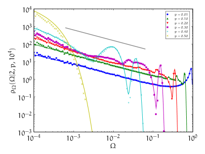
Figure 6: (Color online) Distribution of the frozenness of nodes for different noise strength for RBNs of size $N=10^{5}$ and for $K=2$ and $T=10^{4}$. Each curve was obtained by averaging over 100 different network realizations. The solid lines show the values of $\rho_{\Omega}(\Omega|K=2,p,10^{4})$ according to Eq. (20). The line segment corresponds to a power law with an exponent $0.6$.

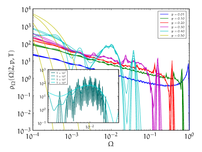
Figure 7: (Color online) Expected distribution of frozenness of each node as function of noise for RBNs with $K=2$ and different values of $T$. The curves represent Eq. (20). The inset shows a zoom into $\rho_{\Omega}(\Omega|K=2,0.4,T)$ for different values of $T$.

The function $\langle\Omega\rangle$ is obtained by performing the integral $\int\Omega\cdot\rho_{\Omega}(\Omega|K=2,p,T)d\Omega$. As can be seen in Figure 4, our calculation of this function agrees well with the results of computer simulations.

IV.4 $K>2$

For larger values of $K$, numerical solutions of Eq. (21) become progressively more elaborate. We did not pursue the task of writing the expressions of 256 function $q_{f}(\{q^{(i)}\})$ for $K=3$ or of $65,536$ functions for $K=4$. Instead, we perform in the following an approximation that is good for a large number of inputs per node.

When $K$ is large, the vast majority of Boolean functions have the output $1$ for approximately half the input combinations. This means that almost all nodes have at their inputs $q$ values close to $1/2$. We therefore make the assumption that the input values to each node are $1$ and $0$ with probability $1/2$, independently from each other. This means that for any given function all input combinations are equally probable. It then follows immediately that the possible $q$ values are identical to the possible fractions of output values 1 in the truth table of a Boolean function, and that the probability for a given $q$ value is

$$p_{q}(q|K,p=0)=2^{-M}{M\choose qM}\,.$$ (24)

Here, we have defined $M=2^{K}$, and the possible $q$ values are thus multiples of $1/M$.

In the presence of noise, each output value is inverted with probability $p$, implying that $q$ is changed to $q^{\prime}=q(1-p)+p(1-q)=(1-2p)q+p$. We therefore have

$$\rho_{q}(q|K,p)=\frac{M}{1-2p}p_{q}\left(\left.\frac{q-p}{1-2p}\right|K,p=0\right)\,.$$ (25)

For the frozenness $\Omega$ we obtain the distribution

$$\rho_{\Omega}(\Omega|K,p)=\frac{M}{2(1-2p)\sqrt{\Omega}}p_{q}\left(\left.\frac{\sqrt{\Omega}+1-p}{2(1-2p)}\right|K,p\right)\,.$$ (26)

Finally, one needs to take into account the effect of fluctuations, exactly as was done for the previous cases,

$$\rho_{q}(q|p,K,T)=\int_{0}^{1}\rho_{q}(q^{\prime}|p,K)\tilde{\rho}_{q}(q|T,q^{\prime})dq^{\prime},$$ (27)

where $\tilde{\rho}_{q}(q|T,q^{\prime})$ is given by Eq. (18).

Fig. 8 shows the distributions of frozenness for $K=4$ and $5$. In contrast to the cases $K=1$ and $K=2$, the peaks are less pronounced, and are hardly visible. For $K=3$ (not shown) there are some peaks which are still visible, specially for high values of $p$. Therefore, the high-$K$ approximation Eq (27) is very good already for $K=4$. Both distributions show the same power-law decay $\rho_{\Omega}(\Omega|K,p)\sim\Omega^{-1/2}$. This is simply due to the fact that for $\Omega\to 0$ ($q\to 1/2$) the shape of $\rho_{q}(q|K,p)$ is essentially flat, and thus $\rho_{\Omega}(\Omega|K,p)\sim dq/d\Omega=\Omega^{-1/2}/2$.

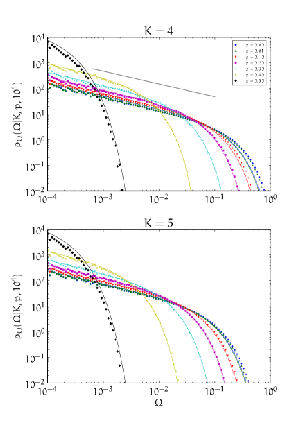
Figure 8: (Color online) Distribution of the frozenness of nodes as function of noise strength for RBN of size $N=10^{4}$ for different values of $K$. Each curve was obtained by averaging the results for 100 different network realizations. The solid lines correspond to Eq. 27.

The quality of our approximation can also be assessed by comparing the analytical prediction for $\left<\Omega\right>$ with the computer simulations (Fig. 4). We expect that the approximation becomes even better for larger $K$.

V Conclusion

We have investigated the effect of thermal noise on RBNs by evaluating two order parameters, the long time average of the Hamming distance between two networks and the average frozenness of the network. While for $K=1$ and $K=2$ the average Hamming distance increases continuously from 0 to 1/2 as $p$ increases from 0 to 1/2, it has a jump at $p=0$ for $K>2$. These findings are well reproduced by the annealed approximation, and they are a consequence of the transition from a frozen to a “chaotic” phase in the deterministic system. In the chaotic phase (occuring for $K>2$), initially nearby trajectories become eventually uncorrelated. The smooth increase of the Hamming distance towards the value 1/2 is compatible with what was found in Miranda and Parga (1989); Qu et al. (2002) for small networks.

The analysis of the average frozenness of the network required more sophisticated calculations than the annealed approximation, and revealed intricate details of the network dynamics. For all values of $K$ the probability distribution of frozenness is a set of delta peaks. For $K=1$, these peaks can be obtained by considering the distance of nodes to nodes with constant functions. For $K>1$, the analysis becomes a lot more elaborate, due to the large number of Boolean functions and the resulting vast number of possible combinations of frozenness values for the inputs of each function. We explained the general method, and performed the actual numerical evaluation for the case $K=2$. The delta peaks show a fractal structure, which emerges from the iterated recursion relation for the possible frozenness values. The variance of the frozenness distribution changes continuously with $p$ for all $K\neq 2$, but for $K=2$ it has a jump at $p=0$, where the variance changes discontinuously from $0$ to a value larger than zero. For larger values of $K$, the delta peaks are so close to each other that the frozenness distribution appears continuous, and in this limit we succeeded in performing an approximate analytical calculation.

We do not find a phase transition at finite noise strength, in contrast to Huepe and Aldana-González (2002), where Boolean networks with threshold functions following a majority rule were used. Such a system undergoes a second order phase transition from an ordered “ferromagnetic” phase, where all nodes assume the same value for the majority of time, to a disordered phase, where the nodes assume both states equally often. The presence of an ordered phase is a direct consequence of the majority rule, and this transition is similar to that in a network of Ising spins Indekeu (2004); Aleksiejuk et al. (2002). The order parameter in Huepe and Aldana-González (2002) was defined as the average “alignment” $s=\left|\left<1-2\sigma\right>\right|$, which is $1$ if all nodes are in the same state. The order parameter $s$ is only meaningful in systems where the system is ordered in the absence of noise, and where the symmetry between the states with values $0$ and $1$ is broken, as in ferromagnetic spin systems. Otherwise, $\left<\Omega\right>$ is a better order parameter, because it captures disordered frozen phases, such as for $K=1$ in RBNs. Of course, a phase transition in the value of $s$ is always accompanied by a phase transition in the value of $\left<\Omega\right>$. The opposite is not always true.

It is to be expected that real networks show some kind of robustness to noise, since they must be able to carry out their function in a noisy environment. As the results of this work show, only for RBNs with $K=1$ do the order parameters change slowly as noise is switched on. RBNs with $K>1$ fail to exhibit robustness to noise, which is hardly surprising given the random wiring of the system and the random choice of functions. It will therefore be interesting to extend the present study to networks with a more restricted set of functions with more biological relevance, such as threshold Szejka et al. (2008) or canalizing functions Moreira and Amaral (2005); Kauffman et al. (2004). At least for some sets of functions, one should expect a phase transition at a finite noise strength, similar to the transition seen in Huepe and Aldana-González (2002). The survival of the “ordered” phase up to a certain noise strength can be viewed as a certain type of robustness.

It remains to be seen how other network topologies Iguchi et al. (2007) and the incorporation of redundancy Gershenson et al. (2006) change a network’s response to noise. In Iguchi et al. (2007), it was shown that a scale-free input distribution changes the average number and length of attractors. In Gershenson et al. (2006), redundancy was introduced as functional duplications of nodes in the network, which resulted in greater robustness against random mutations of the update functions. In both papers, only deterministic dynamics were considered. The effects of these (or other more general) topological and functional characteristics may strongly alter the response of a network to thermal noise. Finding the general conditions required for reliable dynamics in a stochastic environment will be an important step towards a deeper understanding of the dynamical features of real networks.

We acknowledge the support of this work by the Humboldt Foundation.

References

- Kauffman (1969) S. A. Kauffman, J. Theor. Biol. 22, 437 (1969).
- Drossel (2008) B. Drossel, Reviews of Nonlinear Dynamics and Complexity (Wiley, 2008), vol. 1, ISBN 3527407294.
- Rosen-Zvi et al. (2001) M. Rosen-Zvi, A. Engel, and I. Kanter, Phys. Rev. Lett. 87, 078101 (2001).
- Moreira et al. (2004) A. A. Moreira, A. Mathur, D. Diermeier, and L. A. N. Amaral, Proc. Nat. Ac. Sci. 101, 12085 (2004).
- Lagomarsino et al. (2005) M. C. Lagomarsino, P. Jona, and B. Bassetti, Phys. Rev. Lett. 95, 158701 (2005).
- Bornholdt (2005) S. Bornholdt, Science 310, 449 (2005).
- Greil and Drossel (2005) F. Greil and B. Drossel, Phys. Rev. Lett. 95, 048701 (2005).
- Klemm and Bornholdt (2005) K. Klemm and S. Bornholdt, Phys. Rev. E 72, 055101 (2005).
- Samuelsson and Troein (2003) B. Samuelsson and C. Troein, Phys. Rev. Lett. 90, 098701 (2003).
- Drossel (2005) B. Drossel, Phys. Rev. E 72, 016110 (2005).
- Drossel et al. (2005) B. Drossel, T. Mihaljev, and F. Greil, Phys. Rev. Lett. 94, 088701 (2005).
- Shmulevich et al. (2002) I. Shmulevich, E. R. Dougherty, S. Kim, and W. Zhang, Bioinformatics 18, 261 (2002).
- Indekeu (2004) J. O. Indekeu, Physica A 333, 461 (2004).
- Aleksiejuk et al. (2002) A. Aleksiejuk, J. A. Holyst, and D. Stauffer, Physica A 310, 260 (2002).
- McAdams and Arkin (1997) H. H. McAdams and A. Arkin, Proc. Nat. Ac. Sci. 94, 814 (1997).
- Fretter and Drossel (2008) C. Fretter and B. Drossel, Eur. Phys. J. B 62, 365 (2008).
- Miranda and Parga (1989) E. N. Miranda and N. Parga, Europhys. Lett. 10, 293 (1989).
- Golinelli and Derrida (1989) O. Golinelli and B. Derrida, J. Phys 50, 1587 (1989).
- Qu et al. (2002) X. Qu, M. Aldana, and L. P. Kadanoff, J. Stat. Phys. 109, 967 (2002).
- Huepe and Aldana-González (2002) Huepe and Aldana-González, J. Stat. Phys. 108, 527 (2002).
- Derrida and Pomeau (1986) B. Derrida and Y. Pomeau, Europhys. Lett. 1, 45 (1986), ISSN 0295-5075.
- Kaufman and Drossel (2005) Kaufman and Drossel, Eur. Phys. J. B 43, 115 (2005).
- Szejka et al. (2008) A. Szejka, T. Mihaljev, and B. Drossel, New J. Phys. 10, 063009 (2008).
- Moreira and Amaral (2005) A. A. Moreira and L. A. N. Amaral, Phys. Rev. Lett. 94, 218702 (2005).
- Kauffman et al. (2004) S. Kauffman, C. Peterson, B. Samuelsson, and C. Troein, Proc. Nat. Ac. Sci. 101, 17102 (2004).
- Iguchi et al. (2007) K. Iguchi, S. ichi Kinoshita, and H. S. Yamada, J. Theor. Biol. 247, 138 (2007).
- Gershenson et al. (2006) C. Gershenson, S. A. Kauffman, and I. Shmulevich, Artificial Life X: Proceedings of the Tenth International Conference on the Simulation and Synthesis of Living Systems (The MIT Press, 2006), ISBN 0262681625.