$\tilde{\tau}_{1}$ LSP Phenomenology: Two- Versus Four-Body Decay Modes
and Resonant Single Slepton Production at the LHC as an Example

Abstract

We investigate B₃ mSUGRA models, where the lightest stau, $\tilde{\tau}_{1}$, is the LSP. B₃ models allow for lepton number and R-parity violation; the LSP can thus decay. We assume one non-zero B₃ coupling $\lambda^{\prime}_{ijk}$ at $M_{\rm GUT}$, which generates further B₃ couplings at $M_{Z}$. We study the RGEs and give numerical examples. The new couplings lead to additional $\tilde{\tau}_{1}$ decays, providing distinct collider signatures. We classify the $\tilde{\tau}_{1}$ decays and describe their dependence on the mSUGRA parameters. We exploit our results for single slepton production at the LHC. As an explicit numerical example, we investigate single smuon production, focussing on like-sign dimuons in the final state. Also considered are final states with three or four muons.

I Introduction

Supersymmetry Wess:1974tw ; Drees:1996ca ; Nilles:1983ge ; Martin:1997ns (SUSY) is one of the most promising extensions of the Standard Model of particle physics (SM) Glashow:1961tr ; Weinberg:1967tq . In its simplest form, we obtain the supersymmetric Standard Model (SSM), with a doubling of the SM particle content and one extra Higgs doublet. The SSM solves the hierarchy problem of the SM if SUSY is broken at a mass scale $\raise 1.29167pt\hbox{$\;<$\kern-7.5pt\raise-4.73611pt\hbox{$\sim\;$}}{\cal O}(10\,\mathrm{TeV})$. Therefore, SUSY should be testable at the LHC Armstrong:1994it ; CMS:1996fp , which will start taking data this year.

If they exist, supersymmetric particles are typically much heavier than their SM partners and at colliders will mostly decay rapidly. This leads to cascade decay chains in the detector to the lightest supersymmetric particle (LSP). The nature of the LSP and its possible decay modes is thus an essential feature for all supersymmetric signatures. It is the purpose of this paper to study a novel supersymmetric phenomenology, namely with the lightest scalar tau (stau) $\tilde{\tau}_{1}$ as the LSP Allanach:2006st ; Allanach:2003eb . In particular we analyze in detail the potential $\tilde{\tau}_{1}$ decays in baryon-triality, B₃, models Ibanez:1991hv ; Ibanez:1991pr ; Grossman:1998py ; Dreiner:2005rd ; Dreiner:2006xw . We then study the discovery potential of a specific signature in this framework, namely resonant single slepton production at the LHC, resulting in multiple muons in the final state.

I.1 The B₃ Framework

The most general renormalizable superpotential of the SSM is Sakai:1981pk ; Weinberg:1981wj

$$W_{\mathrm{SSM}} = W_{\text{P}_{6}}+W_{\not\text{P}_{6}}\,,$$ (I.1)

$$W_{\text{P}_{6}} = \epsilon_{ab}\left[(\mathbf{Y}_{E})_{ij}L_{i}^{a}H_{d}^{b}\bar{E}_{j}+(\mathbf{Y}_{D})_{ij}Q_{i}^{ax}H_{d}^{b}\bar{D}_{jx}\right.$$ (I.2)

$$\left.+(\mathbf{Y}_{U})_{ij}Q_{i}^{ax}H_{u}^{b}\bar{U}_{jx}+\mu H_{d}^{a}H_{u}^{b}\right],$$

$$W_{\not\text{P}_{6}} = \epsilon_{ab}\left[\frac{1}{2}\lambda_{ijk}L_{i}^{a}L_{j}^{b}\bar{E}_{k}+\lambda^{\prime}_{ijk}L_{i}^{a}Q_{j}^{bx}\bar{D}_{kx}\right]$$ (I.3)

$$+\epsilon_{ab}\kappa^{i}L_{i}^{a}H_{u}^{b}+\frac{1}{2}\epsilon_{xyz}\lambda^{\prime\prime}_{ijk}\bar{U}_{i}^{\,x}\bar{D}_{j}^{\,y}\bar{D}_{k}^{\,z}\,.$$

Here we use the standard notation of Ref. Allanach:1999ic .

The superpotential (I.1) consists of two different parts. $W_{\text{P}_{6}}$, involves the lepton $\mathbf{Y}_{E}$, down-quark $\mathbf{Y}_{D}$, and up-quark ${\bf Y}_{U}$ Yukawa matrices, which give mass to the leptons and quarks after electroweak symmetry breaking.

$W_{\not\text{P}_{6}}$, consists of lepton and baryon number violating operators, which together can lead to rapid proton decay Smirnov:1996bg ; Bhattacharyya:1998bx ; Barbier:2004ez ; Shiozawa:1998si . The SSM thus requires an additional symmetry Dreiner:2005rd ; Ibanez:1991hv ; Ibanez:1991pr to stabilize the proton. The most widely assumed symmetry is R-parity which prohibits $W_{\not\text{P}_{6}}$, leading to the MSSM. But R-parity allows dangerous dimension-five proton decay operators such as $QQQL$ Dimopoulos:1981dw , thus proton-hexality, $\text{P}_{6}$, is preferred Dreiner:2005rd . Here, we consider a third possibility, baryon-triality, $\mathrm{B}_{3}$. $\mathrm{B}_{3}$ is a discrete $\boldsymbol{Z}_{3}$-symmetry which prohibits only the $\bar{U}\bar{D}\bar{D}$ operators in Eq. (I.3) but also the dangerous dimension five operators. See for example Refs. Lee:2007fw ; Lee:2007qx ; Lee:2008pc for $\mathrm{B}_{3}$ models that provide a dark matter candidate.

The $\text{B}_{3}$ SSM has some distinguishing features compared to the MSSM Dreiner:1997uz ; Barbier:2004ez , which can have a strong impact on (hadron) collider phenomenology Dreiner:1991pe ; Allanach:1999bf :

1. Lepton flavor and lepton number are violated.

2. The renormalization group equations (RGEs) get additional contributions Martin:1993zk ; Allanach:1999mh ; Allanach:2003eb .

3. Neutrino masses can be generated as experimentally observed Hall:1983id ; Hempfling:1995wj ; Borzumati:1996hd ; Hirsch:2000ef ; Allanach:2007qc ; Dreiner:2007uj .

4. The LSP is not stable.

5. Supersymmetric particles can be produced singly, possibly on resonance.

Since the LSP is not stable, we are not restricted to the lightest neutralino $\tilde{\chi}_{1}^{0}$ as the LSP Ellis:1983ew . The most general B₃ SSM has more than 200 parameters and in principle any SUSY particle can be the LSP. Within the MSSM, the most widely studied constrained model is minimal supergravity (mSUGRA) with conserved $\text{P}_{6}$ and radiative electroweak symmetry breaking Chamseddine:1982jx ; Barbieri:1982eh ; Hall:1983iz ; Soni:1983rm ; Ibanez:1982fr . The 124 free parameters of the MSSM are reduced to only five

$$M_{0},\,M_{1/2},\,A_{0},\,\tan\beta,\,\text{sgn}(\mu)\,,$$ (I.4)

which are fixed at the grand unification (GUT) scale, $M_{\rm GUT}$. We have a universal scalar mass $M_{0}$, a universal gaugino mass $M_{1/2}$, a universal trilinear scalar coupling $A_{0}$, the ratio of the Higgs vacuum expectation values (vev’s) $\tan\beta$, and the sign of the Higgs mixing parameter $\text{sgn}(\mu)$. For a wide range of these parameters a $\tilde{\chi}_{1}^{0}$ LSP is in fact obtained at the weak scale, $M_{Z}$ Ibanez:1984vq . There are also wide ranges of parameter space with a $\tilde{\tau}_{1}$ LSP, but these are cosmologically excluded in the MSSM or mSUGRA Ellis:1983ew .

In the B₃ mSUGRA model we consider here Allanach:2003eb ; Allanach:2006st , we have six parameters at the GUT scale

$$M_{0},\,M_{1/2},\,A_{0},\,\tan\beta,\,\textnormal{sgn}(\mu),\;\;\text{and}\;\;{\mathbf{\Lambda}^{\prime}},$$ (I.5)

where ${\mathbf{\Lambda}^{\prime}}$ stands for one non-vanishing coupling $\lambda^{\prime}_{ijk}$. A first investigation of the parameter space has shown, that there are extensive regions with a neutralino, a stau or a sneutrino LSP Allanach:2003eb ; Allanach:2006st . We shall focus here on a $\tilde{\tau}_{1}$ LSP. $\tilde{\tau}_{1}$ LSP scenarios have been studied in the literature Akeroyd:1997iq ; deGouvea:1998yp ; Akeroyd:2001pm ; Bartl:2003uq ; Allanach:2003eb ; Allanach:2006st ; Allanach:2007vi ; Dreiner:2007uj ; Bernhardt:2008mz ; steve . As we now discuss, we go beyond this work in several aspects.

I.2 New Phenomenology and Outline

The $\tilde{\tau}_{1}$ LSP might decay via the dominant $L_{i}Q_{j}\bar{D}_{k}$ operator, Eq. (I.3); for example via a 4-body decay in the presence of a non-vanishing $\lambda^{\prime}_{211}$

$$\tilde{\tau}^{-}_{1}\overset{\lambda^{\prime}_{211}}{\longrightarrow}\tau^{-}\mu^{-}u\bar{d}\,.$$ (I.6)

An important feature of B₃ mSUGRA models is that additional $\mathrm{B}_{3}$ couplings are generated via the RGE running. These new couplings can lead to 2-body decays of the $\tilde{\tau}_{1}$ LSP. For example, $\lambda^{\prime}_{211}$ will generate $\lambda_{233}$ which allows for the decay

$$\tilde{\tau}_{1}^{-}\overset{\lambda_{233}}{\longrightarrow}\mu^{-}\nu_{\tau}\,.$$ (I.7)

Even though $\lambda_{233}\ll\lambda_{211}^{\prime}$, this might be the dominant decay mode. The decay (I.6) is suppressed by phase space and heavy propagators.

We analyze in detail the conditions for a dominance of the 2-body decay over the 4-body decay. We provide for the first time an extensive study of $\mathrm{B}_{3}$ $\tilde{\tau}_{1}$ LSP decays and extend and specify thus the results of steve , where a first estimate has been performed. This is useful when studying both pair produced and singly produced SUSY particles within the $\mathrm{B}_{3}$ mSUGRA model. Typically all heavy SUSY particle decay to the ($\tilde{\tau}_{1}$) LSP.

In the second half of our paper, we consider the $\mathrm{B}_{3}$ mSUGRA model with a $\tilde{\tau}_{1}$ LSP and focus on resonant single (left-handed) charged slepton $\tilde{\ell}_{Li}$ and sneutrino $\tilde{\nu}_{i}$ production at hadron colliders, which proceeds via a dominant $L_{i}Q_{j}\bar{D}_{k}$ operator:

$$\bar{u}_{j}d_{k} \overset{\lambda^{\prime}_{ijk}}{\longrightarrow} \tilde{\ell}^{-}_{Li}\,,$$ (I.8)

$$\bar{d}_{j}d_{k} \overset{\lambda^{\prime}_{ijk}}{\longrightarrow} \tilde{\nu}_{i}.$$ (I.9)

Here, $u_{j}$ ($d_{k}$) is an up-type (down-type) quark of generation $j$ ($k$).

Single slepton production allows us also to study two $\mathrm{B}_{3}$ couplings at a time, depending on the scenario. The slepton is always produced via a $\lambda^{\prime}$ whereas the decay of the $\tilde{\tau}_{1}$ LSP in the decay chain of the slepton might proceed via a generated $\lambda$, cf. Eq. (I.7).

Single slepton production within a $\tilde{\chi}_{1}^{0}$ LSP scenario leads to like-sign dileptons in the final state and has thus a very promising signature for experimental studies, see Refs. Dreiner:2000vf ; Dreiner:2000qf ; Dreiner:1998gz ; Moreau:2000bs ; Deliot:2000mf . Here we show that for a $\tilde{\tau}_{1}$ LSP, we also obtain like-sign dilepton events and additionally events with three or four leptons in the final state. We give event rates for the LHC for two representative sets of $\mathrm{B}_{3}$ mSUGRA parameters. We also discuss the background, although a detailed signal over background analysis is beyond the scope of this paper. This is the first study of single slepton production in $\tilde{\tau}_{1}$ LSP scenarios.

We assume in the following that only one non-vanishing $\lambda^{\prime}_{ijk}$ is present at $M_{\mathrm{GUT}}$, similar to the dominant top Yukawa in the SM. Allowing for more than one coupling leads to stricter bounds Dreiner:1997uz ; Barbier:2004ez ; Chemtob:2004xr ; Dreiner:2006gu ; Allanach:1999ic ; Agashe:1995qm . The bounds for a single $\lambda^{\prime}_{ijk}$ lie between $\mathcal{O}(1)$ and $\mathcal{O}(10^{-4})$ depending on the flavor indices and sparticle masses. These bounds can be up to four orders of magnitude stronger at $M_{\rm GUT}$ if one includes the generation of neutrino masses Allanach:1999ic ; Allanach:2003eb . We therefore assume below that $\lambda^{\prime}_{ijk}\raise 1.29167pt\hbox{$\;<$\kern-7.5pt\raise-4.73611pt\hbox{$\sim\;$}}\mathcal{O}(10^{-2})$ and require it to be consistent with the observed neutrino masses.

Resonant slepton production at hadron colliders via the $L_{i}Q_{j}\bar{D}_{k}$ operator was first investigated in Dimopoulos:1988jw ; Dimopoulos:1988fr , using tree-level production cross sections. Three-lepton final states and like-sign dilepton events were investigated in Ref. Dreiner:2000vf ; Dreiner:2000qf ; Dreiner:1998gz ; Moreau:2000bs ; Deliot:2000mf . Ref. Allanach:2003wz considered scenarios with a gravitino LSP. Experimental studies by the D0 collaboration at the Tevatron were performed in Refs. Abazov:2002es ; Abazov:2006ii assuming a $\tilde{\chi}_{1}^{0}$ LSP and a non-vanishing $\lambda^{\prime}_{211}$. The NLO QCD corrections to the cross section were computed in Choudhury:2002au ; Yang:2005ts ; Dreiner:2006sv ; Chen:2006ep . The SUSY-QCD corrections were included by Dreiner:2006sv . The latter can modify the NLO QCD prediction by up to 35%. In Refs. Bernhardt:2008mz ; Borzumati:1999th ; Accomando:2006ga ; Belyaev:2004qp single slepton production in association with a single top quark was considered.

The outline of our paper is as follows. In Sect. II we review the $\mathrm{B}_{3}$ mSUGRA model and approximate formulæ for sparticle masses. We define two $\mathrm{B}_{3}$ mSUGRA scenarios with a $\tilde{\tau}_{1}$ LSP, as a reference for phenomenological studies. We then derive approximate equations for the RGE generation of $\lambda$ from $\lambda^{\prime}$. In Sect. III, we classify the different decay modes of the $\tilde{\tau}_{1}$ LSP and investigate the conditions for a dominance of the 2-body decay over the 4-body decay and vice versa. In Sect. IV, we classify all possible signatures for resonant single slepton production in $\mathrm{B}_{3}$ mSUGRA models with a $\tilde{\tau}_{1}$ LSP. In Sect. V we calculate event rates for like-sign dimuon events as well as for three- and four-muon events, at the LHC. We also discuss backgrounds and cuts for like-sign dimuon events. We conclude in Sect. VI.

II The low energy spectrum of the $\mathrm{B}_{3}$ mSUGRA Model with a $\tilde{\tau}_{1}$ LSP

We have defined the $\mathrm{B}_{3}$ mSUGRA model in Eq. (I.5) via six input parameters at the GUT scale Allanach:2003eb ; Allanach:2006st . We now discuss the low energy spectrum. Sparticle masses and couplings are obtained by running the respective RGEs down to the weak scale. Due to the mixing of different quark flavors, described by the Cabibbo-Kobayashi-Maskawa (CKM) matrix, the RGEs of the $\mathrm{B}_{3}$ couplings are not independent, but highly coupled. Therefore, a single non-zero $\lambda^{\prime}_{ijk}$ at the GUT scale generates a set of other non-zero $\mathrm{B}_{3}$ couplings at lower scales. Assuming a diagonal charged lepton Yukawa matrix $\mathbf{Y}_{E}$, only those couplings can be generated which violate the same lepton number as $\lambda^{\prime}_{ijk}$, i.e. $\lambda^{\prime}_{imn}$ and $\lambda_{ill}$. No additional source of lepton number violation is introduced. Phenomenologically particularly relevant is the generation of $\lambda_{i33}$, which we discuss in detail in Sect. II.4.

II.1 Sparticle Spectra

The low energy SUSY particle masses depend strongly on the universal mSUGRA parameters (I.4) and only weakly on $\lambda^{\prime}\raise 1.29167pt\hbox{$\;<$\kern-7.5pt\raise-4.73611pt\hbox{$\sim\;$}}\mathcal{O}(10^{-2})$ Allanach:2006st . For later use, we cite here approximate expressions for the relevant SUSY particle masses in terms of the mSUGRA parameters as given in Drees:1995hj , cf. also the original work in Ref. Ibanez:1984vq . The masses of the sleptons of the first and second generation are

$$\begin{split}m_{\tilde{\ell}_{R}}^{2}&=M_{0}^{2}+0.15M_{1/2}^{2}-\sin^{2}\theta_{W}M_{Z}^{2}\cos 2\beta,\\ m_{\tilde{\ell}_{L}}^{2}&=M_{0}^{2}+0.52M_{1/2}^{2}-(0.5-\sin^{2}\theta_{W})M_{Z}^{2}\cos 2\beta,\\ m_{\tilde{\nu}}^{2}&=M_{0}^{2}+0.52M_{1/2}^{2}+0.5M_{Z}^{2}\cos 2\beta,\end{split}$$ (II.10)

where $m_{\tilde{\ell}_{R,L}}$ denotes the mass of a right-/left-handed selectron or smuon, respectively, $m_{\tilde{\nu}}$ the mass of a left-handed electron or muon sneutrino, and $\theta_{W}$ the electroweak mixing angle. $M_{Z}$ is the mass of the $Z$ boson.

For sfermions of the third generation, the mixing between left- and right-handed gauge-current eigenstates has to be taken into account. The stau mass matrix squared $\mathfrak{M}^{2}_{\tilde{\tau}}$ is given by Gunion:1984yn

$$\mathfrak{M}^{2}_{\tilde{\tau}} =\left({m_{\tau}^{2}+A_{LL}\qquad m_{\tau}B_{LR}}\atop{m_{\tau}B_{LR}\qquad m_{\tau}^{2}+C_{RR}}\right),$$ (II.11)

with $m_{\tau}$ denoting the tau lepton mass and, expressed in terms of left- and right-handed third generation softbreaking parameters $m_{\tilde{L}_{3}}$ and $m_{\tilde{E}_{3}}$, respectively,

$$\begin{split}A_{LL}&=m^{2}_{\tilde{L}_{3}}-(0.5-\sin^{2}\theta_{W})M_{Z}^{2}\cos 2\beta\,,\\ B_{LR}&=A_{\tau}-\mu\tan{\beta}\,,\\ C_{RR}&=m^{2}_{\tilde{E}_{3}}-\sin^{2}\theta_{W}M_{Z}^{2}\cos 2\beta,\end{split}$$ (II.12)

where $A_{\tau}$ is the trilinear coupling of the left- and right-handed stau to the Higgs. In mSUGRA, $A_{\tau}=A_{0}$ at the GUT scale. The softbreaking parameters depend on the mSUGRA parameters as follows Drees:1995hj ,

$$m_{\tilde{E}_{3}}^{2} =M_{0}^{2}+0.15M_{1/2}^{2}-\frac{2}{3}X_{\tau},$$

$$m_{\tilde{L}_{3}}^{2} =M_{0}^{2}+0.52M_{1/2}^{2}-\frac{1}{3}X_{\tau},$$ (II.13)

$$X_{\tau} \equiv 10^{-4}(1+\tan^{2}\beta)\left(M_{0}^{2}+0.15M_{1/2}^{2}+0.33A_{0}^{2}\right),$$

where $X_{\tau}$ parameterizes the influence of the tau Yukawa coupling. Note, that $X_{\tau}$ can have a strong impact on the stau masses due to its $\tan^{2}\beta$ dependence, even though $X_{\tau}$ is suppressed by a factor $10^{-4}$. We will investigate this effect on the $\tilde{\tau}_{1}$ decay branching ratios in the next section.

The stau mass eigenstates $\tilde{\tau}_{1,2}$ are obtained from the gauge eigenstates by a unitary rotation $U$ such that $U$ diagonalizes the mass matrix, $U\mathfrak{M}^{2}_{\tilde{\tau}}U^{\dagger}\,=\,\text{diag}\left(m_{\tilde{\tau}_{1}}^{2},m_{\tilde{\tau}_{2}}^{2}\right)$, yielding for the masses $m_{\tilde{\tau}_{1,2}}$

$$\begin{split}m_{\tilde{\tau}_{1,2}}^{2}=&\,m_{\tau}^{2}+\frac{1}{2}(A_{LL}+C_{RR})\\ &\mp\frac{1}{2}\sqrt{(A_{LL}-C_{RR})^{2}+4m_{\tau}^{2}B_{LR}^{2}}\,.\end{split}$$ (II.14)

The gaugino masses can be approximated in terms of the universal gaugino mass $M_{1/2}$ Drees:1995hj ,

$$\begin{split}m_{\tilde{\chi}_{1}^{0}}&\simeq M_{1}=0.41M_{1/2},\\ m_{\tilde{\chi}_{2}^{0}}&\simeq M_{2}=0.84M_{1/2}.\end{split}$$ (II.15)

Here it has been used that the lightest neutralino $\tilde{\chi}_{1}^{0}$ is bino-like in many mSUGRA models and that its mass can be approximated by the bino mass parameter $M_{1}$ at the weak scale. Accordingly, the second lightest neutralino $\tilde{\chi}_{2}^{0}$ is mainly wino-like and its mass governed by the wino mass parameter $M_{2}$.

II.2 Reference Scenarios with a $\tilde{\tau}_{1}$ LSP

For the purpose of numerical studies and as future reference points, we define two specific sets of $\mathrm{B}_{3}$ mSUGRA scenarios with a $\tilde{\tau}_{1}$ LSP:

$$\begin{split}\textnormal{\bf Set A:\,\,}&M_{0}=0\textnormal{\,GeV},\,M_{1/2}=500\textnormal{\,GeV},\\ &A_{0}=600\textnormal{\,GeV},\,\tan\beta=13,\textnormal{sgn}(\mu)=+1,\\ &\textnormal{a single\,}\lambda^{\prime}_{ijk}\neq 0\lvert_{\rm GUT},\\[8.61108pt] \textnormal{\bf Set B:\,\,}&M_{0}=0\textnormal{\,GeV},\,M_{1/2}=700\textnormal{\,GeV},\\ &A_{0}=1150\textnormal{\,GeV}\,,\tan\beta=26,\textnormal{sgn}(\mu)=+1,\\ &\textnormal{a single\,}\lambda^{\prime}_{ijk}\neq 0\lvert_{\rm GUT}.\end{split}$$ (II.16)

They are chosen in accordance with the following bounds :

• ${\rm BR}(B_{s}\rightarrow\mu^{+}\mu^{-})<5.8\times 10^{-8}$ at the $95\%$ C.L. obtained by the CDF collaboration :2007kv .

• $2.76\times 10^{-4}<{\rm BR}(b\rightarrow s\gamma)<4.34\times 10^{-4}$ which is the central theoretical value at $2\sigma$ Allanach:2006st using the experimental value of Barberio:2007cr .

• The discrepancy between experiment and the SM prediction of the anomalous magnetic moment of the muon is $\delta a_{\mu}=a_{\mu}^{\rm exp}-a_{\mu}^{\rm SM}=(29.5\pm 8.8)\times 10^{-10}$, i.e. $3.4\sigma$ Bennett:2006fi ; Miller:2007kk ; Stockinger:2007pe . The sets (II.16) are chosen such that $\delta a_{\mu}^{\rm SUSY}=a_{\mu}^{\rm MSSM}-a_{\mu}^{\rm SM}$ agrees with $\delta a_{\mu}$ within $2\sigma$.

• Higgs mass $m_{h^{0}}\geq 112.4$ GeV. This value corresponds to the LEPII bound of $m_{h^{0}}\geq 114.4$ GeV at $95\%$ C.L. Barate:2003sz assuming a numerical error of 2 GeV for the mass prediction.

• A non-vanishing coupling $\lambda^{\prime}_{ijk}$ at the GUT scale will generate a tree-level neutrino mass Hall:1983id ; Ellis:1984gi ; deCarlos:1996du ; Nardi:1996iy ; Allanach:2003eb . All couplings $\lambda^{\prime}_{ijk}$ in the following are chosen such that the tree-level neutrino mass is smaller than the cosmological bound on the sum of neutrino masses from WMAP Spergel:2003cb combined with 2dGRFS data Colless:2003wz : $\sum_{i}m_{\nu_{i}}<0.71$ eV. A corresponding comprehensive set of bounds for the mSUGRA parameter set SPS1a Allanach:2002nj with one non-vanishing coupling $\lambda^{\prime}_{ijk}$ is given in Ref. Allanach:2003eb . Note, that the generated tree-level neutrino mass depends on all mSUGRA parameters (I.5). The neutrino mass bounds on $\lambda^{\prime}_{ijk}$ for Set A and Set B are weaker compared to those for SPS1a.

We use the computer programs provided by onlinecalc ; Allanach:2003jw ; Belanger:2005jk to calculate ${\rm BR}(B_{s}\rightarrow\mu^{+}\mu^{-})$, ${\rm BR}(b\rightarrow s\gamma)$, and $\delta a_{\mu}^{\rm SUSY}$. These programs do not include the B₃ couplings. But the corresponding effects are negligible for $\lambda^{\prime}_{ijk}\raise 1.29167pt\hbox{$\;<$\kern-7.5pt\raise-4.73611pt\hbox{$\sim\;$}}\mathcal{O}(10^{-2})$ Allanach:2006st .

	masses [GeV]			masses [GeV]
	Set A	Set B		Set A	Set B
$\tilde{\tau}_{1}$	179	146	$\tilde{\chi}_{1}^{0}$	203	290
$\tilde{e}_{R}$	193	266	$\tilde{\chi}_{2}^{0}$	380	544
$\tilde{\tau}_{2}$	340	453	$\tilde{\chi}_{3}^{0}$	571	754
$\tilde{e}_{L}$	340	471	$\tilde{\chi}_{4}^{0}$	587	765
$\tilde{\nu}_{\tau}$	326	437	$\tilde{\chi}_{1}^{\pm}$	383	549
$\tilde{\nu}_{e}$	329	461	$\tilde{\chi}_{2}^{\pm}$	583	761
$\tilde{t}_{1}$	841	1160	$h^{0}$	113	115
$\tilde{b}_{1}$	970	1300	$H^{0}$	643	795
$\tilde{u}_{R}$	1010	1370	$A^{0}$	642	795
$\tilde{t}_{2}$	1010	1340	$H^{+}$	648	799
$\tilde{b}_{2}$	995	1340
$\tilde{u}_{L}$	1040	1410	$\tilde{g}$	1150	1560

Table 1: Sparticle masses for the $\mathrm{B}_{3}$ mSUGRA sets A and B as defined in Eq. (II.16), evaluated for a renormalization scale $Q_{\rm susy}=\sqrt{m_{\tilde{t}_{1}}(Q_{\rm susy})\,m_{\tilde{t}_{2}}(Q_{\rm susy})}$ using Softsusy 2.0.10 Allanach:2001kg . The variation due to different $\lambda^{\prime}_{ijk}\neq 0|_{\rm GUT}$ and quark mixing (see Sect. II.3) is below the percent level. The masses in the second generation coincide with those in the first generation.

We show in Table 1 the supersymmetric mass spectra of the parameter sets A and B (II.16). We have neglected the mass dependence on the different non-zero B₃ couplings which is valid if $\lambda^{\prime}_{ijk}\raise 1.29167pt\hbox{$\;<$\kern-7.5pt\raise-4.73611pt\hbox{$\sim\;$}}\mathcal{O}(10^{-2})$ Allanach:2006st . The main B₃ effect on the spectrum is that we allow for a $\tilde{\tau}_{1}$ LSP.

One naturally obtains a $\tilde{\tau}_{1}$ LSP spectrum for $M_{1/2}\gg M_{0}$. The large $M_{1/2}$ raises the lightest neutralino mass (II.15) faster than the right-handed slepton masses (II.10). It also drives the gluino and indirectly via the RGEs the squark masses up. We thus see in Table 1 squark and gluino masses $\raise 1.29167pt\hbox{$\;>$\kern-7.5pt\raise-4.73611pt\hbox{$\sim\;$}}1\,$TeV, while the slepton masses are below 500 GeV. Another general feature of a $\tilde{\tau}_{1}$ LSP scenario is that the second lightest neutralino and the lightest chargino are also heavier than the sleptons. Therefore the only conventional supersymmetric decays of the left-handed sleptons are via the lightest neutralino. Depending on the dominant B₃ coupling and its size, the left-handed sleptons can also decay into two jets.

Nearly all sparticles in Set B ($M_{1/2}=700$ GeV) are heavier than in Set A ($M_{1/2}=500$ GeV). The most important difference for the phenomenology at colliders arises from the different values of $\tan\beta$ ($\tan\beta=13$ in Set A, $\tan\beta=26$ in Set B). According to Eq. (II.13), the soft breaking parameters of the stau decrease for increasing $\tan\beta$ and thus both stau mass eigenstates are reduced for large values of $\tan\beta$. Furthermore, the mass of the lighter stau is reduced due to the larger L–R-mixing, cf. Eq. (II.11). This effect can be seen in Table 1, where the mass of the $\tilde{\tau}_{1}$ LSP is 179 GeV in Set A but only 146 GeV in Set B. The $\tilde{\tau}_{1}$ mass and $\tan\beta$ strongly influence the possible 2- and 4-body $\tilde{\tau}_{1}$ LSP branching ratios. We will investigate this topic in detail in Sect. III.

II.3 Fermion Mixing

Since the B₃ RGEs are coupled, given one non-zero B₃ coupling at $M_{\rm GUT}$, we will generate many non-zero couplings at the weak scale $M_{Z}$. As we will see in the next section, the size of the dynamically generated B₃ couplings depends sensitively on the composition of the quark Yukawa matrices. For this reason we prepend here a short discussion of quark mixing in B₃ models.

Initially at $M_{\rm GUT}$, all parameters are given in the weak-current eigenstate basis. This includes the quark and lepton Yukawa coupling matrices ${\bf Y}_{U},\,{\bf Y}_{D},\,{\bf Y}_{E}$ and the corresponding mass matrices $\bf{m}_{u},\,\bf{m}_{d},\,\bf{m}_{e}$. Since, in general, these matrices are not diagonal, we need to rotate the (charged) lepton and quark fields from the weak into the mass eigenstate basis,

$$f_{L,R}^{\rm mass} ={\bf V_{f\,L,R}}\,\,f_{L,R}^{\rm weak}\,,$$ (II.17)

with $f_{L,R}$ denoting the left- and right-handed fermion fields, respectively and $\bf V_{f\,L,R}$ denoting the corresponding rotation matrices. The mass matrices in the mass eigenstate basis are then given by

$$\begin{split}\bf{V_{u\,L}}\,\bf{m}_{u}\,\bf{V_{u\,R}^{+}}&=\text{diag}(m_{u},m_{c},m_{t}),\\ \bf{V_{d\,L}}\,\bf{m}_{d}\,\bf{V_{d\,R}^{+}}&=\text{diag}(m_{d},m_{s},m_{b}),\\ \bf{V_{e\,L}}\,\bf{m}_{e}\,\bf{V_{e\,R}^{+}}&=\text{diag}(m_{e},m_{\mu},m_{\tau}),\end{split}$$ (II.18)

defined at the weak scale $M_{Z}$. The rotation matrices ${\bf V_{f\,L,R}}$ are not directly experimentally accessible but only the CKM matrix $\bf V_{\rm CKM}$,

$$\bf V_{\rm CKM}=V_{u\,L}V_{d\,L}^{+}.$$ (II.19)

In general, the rotation matrices for the left-handed fields differ from those for the right-handed fields. In the following, however, for simplicity and definiteness, we assume real and symmetric Yukawa coupling matrices, thus $\bf V_{f\,L}=V_{f\,R}$. Furthermore we neglect neutrino masses in this context and assume that ${\bf Y}_{E}$ is diagonal in the weak-current basis. Correspondingly, ${\bf V_{e\,L,R}}=\mathbf{1}_{3\times 3}$.

To further constrain the quark Yukawa couplings, we restrict ourselves to the extreme cases of quark mixing taking place completely in the up- or the down-quark sector, respectively. We will refer to it as “up-type mixing” if

$${\bf V_{u\,L,R}}={\bf V_{\rm CKM}},\quad{\bf V_{d\,L,R}}={\bf 1}_{3\times 3},$$ (II.20)

at the weak scale $M_{Z}$ and as “down-type mixing” if

$${\bf V_{u\,L,R}}={\bf 1}_{3\times 3},\quad{\bf V_{d\,L,R}}={\bf V_{\rm CKM}^{+}}$$ (II.21)

at the weak scale. Therefore, in up-type mixing scenarios, the Yukawa matrices are

$${\bf Y}_{U}(M_{Z})\times v_{u} ={\bf V_{\rm CKM}^{+}}\cdot\text{diag}(m_{u},m_{c},m_{t})\cdot{\bf V_{\rm CKM}},$$

$${\bf Y}_{D}(M_{Z})\times v_{d} =\text{diag}(m_{d},m_{s},m_{b}),$$ (II.22)

and in down-type mixing scenarios, the Yukawa matrices are

$${\bf Y}_{U}(M_{Z})\times v_{u} =\text{diag}(m_{u},m_{c},m_{t}),$$ (II.23)

$${\bf Y}_{D}(M_{Z})\times v_{d} ={\bf V_{\rm CKM}}\cdot\text{diag}(m_{d},m_{s},m_{b})\cdot{\bf V_{\rm CKM}^{+}},$$

respectively. In the following we will consider these two extreme cases. $v_{u}$ ($v_{d}$) is the vacuum expectation value of the up-type (down-type) neutral CP-even Higgs with

$$v_{u}=v\sin\beta\,,\quad\quad v_{d}=v\cos\beta\,,$$ (II.24)

where $v=174$ GeV is the SM vacuum expectation value .

As a consequence of the non-trivial quark rotation matrices, the $\lambda^{\prime}_{ijk}$ coupling in Eq. (I.5) also has to be rotated from the weak basis into the quark mass basis for a comparison with experimental data. In case of up-type mixing, the $L_{i}Q_{j}\bar{D}_{k}$ interactions of the superpotential (I.1) in the quark mass basis are in terms of SU(2) component superfields

$$\lambda^{\prime}_{ijk}[N_{i}D^{m}_{j}-E_{i}{\bf(V_{\rm CKM}^{+}})_{jl}U^{m}_{l}]\bar{D}^{m}_{k}\,.$$ (II.25)

In the case of down-mixing they are

$$\lambda^{\prime}_{ijk}[N_{i}{\bf(V_{\rm CKM}})_{jl}D^{m}_{l}-E_{i}U^{m}_{j}]{\bf(V_{\rm CKM}^{+}})_{nk}\bar{D}^{m}_{n}\,.$$ (II.26)

See also Ref. Agashe:1995qm . However for slepton production cross sections, we do not take into account these CKM effects. If needed, the corresponding rescaling of the $\lambda^{\prime}$ coupling can be done easily. Furthermore the sub-dominant interactions, which include non-diagonal matrix elements of ${\bf V_{\rm CKM}}$, do not allow for large production cross sections since $\lambda^{\prime}$ enters only quadratically.

II.4 Renormalization Group Equations

One of the most important consequence of including $\mathrm{B}_{3}$ effects in SUSY models is that the LSP is no longer stable. This is of special interest for phenomological studies if the LSP couples directly to the dominant $\mathrm{B}_{3}$ operator. This leads to large LSP decay widths and to distinctive final state signatures.

In the scenarios considered in this work, cf. Eq. (I.5), the dominant coupling is a $\lambda^{\prime}_{ijk}$; for $i\neq 3$ it does not couple to the $\tilde{\tau}_{1}$ LSP. However, the RGEs of the $\mathrm{B}_{3}$ couplings are coupled via non-diagonal entries of Higgs-Yukawa matrices and a $\lambda^{\prime}_{ijk}$ generates dynamically other $\mathrm{B}_{3}$ couplings. Among those, we want to focus on the $\lambda_{i33}$ which do couple directly to the $\tilde{\tau}_{1}$ LSP.

The aim of the next two sections is to study the RGEs of the dominant $\lambda^{\prime}_{ijk}$ and to quantitatively determine the generated $\lambda_{i33}$. We then use these results to predict the low energy spectrum of $\mathrm{B}_{3}$ mSUGRA scenarios given by Eq. (I.5). We will also derive approximate formulæ that allow for a numerical implementation of the running of the couplings.

The full renormalization group equations for the $\mathrm{B}_{3}$ couplings $\lambda^{\prime}_{ijk}$ and $\lambda_{i33}$ are Martin:1993zk ; Allanach:2003eb ; Allanach:1999mh ,

$$\begin{split}16\pi^{2}\frac{d}{dt}\lambda^{\prime}_{ijk}=\,&\lambda^{\prime}_{ijl}\,\gamma_{D_{l}}^{D_{k}}+\lambda^{\prime}_{ilk}\,\gamma_{Q_{l}}^{Q_{j}}+\lambda^{\prime}_{ljk}\,\gamma_{L_{l}}^{L_{i}}\\ &-\big{(}\mathbf{Y}_{D}\big{)}_{jk}\,\gamma_{H_{1}}^{L_{i}},\end{split}$$ (II.27)

$$\begin{split}16\pi^{2}\frac{d}{dt}\lambda_{i33}=\,&\lambda_{i3l}\,\gamma_{E_{l}}^{E_{3}}+\lambda_{il3}\,\gamma_{L_{l}}^{L_{3}}+\lambda_{l33}\,\gamma_{L_{l}}^{L_{i}}\\ &-\big{(}\mathbf{Y}_{E}\big{)}_{33}\,\gamma_{H_{1}}^{L_{i}}+\big{(}\mathbf{Y}_{E}\big{)}_{i3}\,\gamma_{H_{1}}^{L_{3}},\end{split}$$ (II.28)

with $t=\ln Q$, $Q$ being the renormalization scale. The anomalous dimensions $\gamma$ are listed in Allanach:2003eb at one-loop level and in Allanach:1999mh at two-loop level. The RGEs simplify considerably under the assumption of the single $\mathrm{B}_{3}$ coupling dominance hypothesis Dimopoulos:1988jw ; Barger:1989rk . Products of two or more $\mathrm{B}_{3}$ couplings including quadratic contributions of the dominant coupling can be neglected for $\lambda^{\prime}\raise 1.29167pt\hbox{$\;<$\kern-7.5pt\raise-4.73611pt\hbox{$\sim\;$}}\mathcal{O}(10^{-2})$. In this limit, the one-loop anomalous dimensions read

$$\begin{split}\gamma_{Q_{j}}^{Q_{i}}=\,&\big{(}\mathbf{Y}_{D}\mathbf{Y}_{D}^{+}\big{)}_{ij}+\big{(}\mathbf{Y}_{U}\mathbf{Y}_{U}^{+}\big{)}_{ij}\\ &-\delta_{j}^{i}\Big{(}\frac{1}{30}g_{1}^{2}+\frac{3}{2}g_{2}^{2}+\frac{8}{3}g_{3}^{2}\Big{)},\\ \gamma_{D_{j}}^{D_{i}}=\,&2\big{(}\mathbf{Y}_{D}^{+}\mathbf{Y}_{D}\big{)}_{ji}-\delta_{j}^{i}\Big{(}\frac{2}{15}g_{1}^{2}+\frac{8}{3}g_{3}^{2}\Big{)},\\ \gamma_{L_{j}}^{L_{i}}=\,&\big{(}\mathbf{Y}_{E}\mathbf{Y}_{E}^{+}\big{)}_{ij}-\delta_{j}^{i}\Big{(}\frac{3}{10}g_{1}^{2}+\frac{3}{2}g_{2}^{2}\Big{)},\\ \gamma_{E_{j}}^{E_{i}}=\,&2\big{(}\mathbf{Y}_{E}^{+}\mathbf{Y}_{E}\big{)}_{ji}-\delta_{j}^{i}\Big{(}\frac{6}{5}g_{1}^{2}\Big{)},\\ \gamma_{H_{1}}^{L_{i}}=\,&-3\lambda^{\prime}_{iaq}\big{(}\mathbf{Y}_{D}\big{)}_{aq}-\lambda_{ibq}\big{(}\mathbf{Y}_{E}\big{)}_{bq}\,,\end{split}$$ (II.29)

where $g_{1},\,g_{2},\,g_{3}$ are the three gauge couplings.

From Eqs. (II.28) and (II.29), we see that the terms related to $\gamma_{H_{1}}^{L_{i}}$ allow for the dynamical generation of $\lambda_{i33}$ by a non-zero $\lambda^{\prime}_{iaq}$ coupling [and vice versa for Eq. (II.27)]. All other terms in Eq. (II.28) only alter the running of $\lambda_{i33}$ once it is generated. The RGEs can be further simplified. At one-loop level, all $\mathrm{B}_{3}$ couplings but the dominant $\lambda^{\prime}_{ijk}$ and the generated $\lambda_{i33}$ can be neglected in the RGEs since they must be generated first by $\lambda^{\prime}$ and thus contribute at two-loop level only.

Since we work in a diagonal charged lepton Yukawa basis, the last term in Eq. (II.28), proportional to $\big{(}\mathbf{Y}_{E}\big{)}_{i3}$ does not contribute to the running of $\lambda_{i33}$. It is only non-zero if $i=3$, but owing to the $ij$-antisymmetry of $\lambda_{ijk}$ no coupling is generated in this case ($\lambda_{333}=0$).

Next, a general ordering of the parameters in the anomalous dimensions is

$$g_{3}^{2}>\big{(}\mathbf{Y}_{U}\big{)}_{33}^{2}>g_{2}^{2}>g_{1}^{2}>\big{(}\mathbf{Y}_{D}\big{)}_{33}^{2}>\big{(}\mathbf{Y}_{E}\big{)}_{33}^{2},$$ (II.30)

and all other entries of the $\mathbf{Y}$ matrices are smaller by at least one order of magnitude . The contributions to the RGEs are thus largest for diagonal anomalous dimensions.

As a result, the RGEs for a non-zero $\lambda^{\prime}_{ijk}$ at the GUT scale and a generated $\lambda_{i33}$ reduce to

$$\begin{split}16\pi^{2}\frac{d}{dt}\lambda^{\prime}_{ijk}=\,&\lambda^{\prime}_{ijk}\,\Big{[}-\frac{7}{15}g_{1}^{2}-3g_{2}^{2}-\frac{16}{3}g_{3}^{2}\\ &+\big{(}\mathbf{Y}_{D}\big{)}_{33}^{2}\big{(}2\delta_{k3}+\delta_{j3}+3\delta_{j3}\delta_{k3}\big{)}\\ &+\big{(}\mathbf{Y}_{U}\big{)}_{33}^{2}\delta_{j3}+\big{(}\mathbf{Y}_{E}\big{)}_{33}^{2}\delta_{i3}\Big{]},\end{split}$$ (II.31)

$$\begin{split}16\pi^{2}\frac{d}{dt}\lambda_{i33}=\,&\lambda_{i33}\,\Big{[}-\frac{9}{5}g_{1}^{2}-3g_{2}^{2}+4\big{(}\mathbf{Y}_{E}\big{)}_{33}^{2}\Big{]}\\ &+3\lambda^{\prime}_{ijk}\big{(}\mathbf{Y}_{E}\big{)}_{33}\big{(}\mathbf{Y}_{D}\big{)}_{jk}\,.\end{split}$$ (II.32)

A similar analytical approximation for the generation of $\lambda$ is derived in steve . But the effect of the gauge couplings is neglected there. See also Ref. deCarlos:1996du .

The last term in Eq. (II.32) induces the dynamical generation of $\lambda_{i33}$. Diagrammatically, this process can be understood as shown in Fig. 1. We see that at one-loop the lepton-doublet superfield mixes with the Higgs doublet superfield $H_{d}$ via the $\mathrm{B}_{3}$ coupling $\lambda^{\prime}_{ijk}$ and the standard down quark Yukawa coupling. $H_{d}$ then couples via the tau Yukawa coupling $\big{(}\mathbf{Y}_{E}\big{)}_{33}$ purely leptonically. The resulting effective interaction is of the $\lambda_{i33}$-type.

Figure 1: Superfield diagram for the dynamical generation of $\lambda_{i33}$ by $\lambda^{\prime}_{ijk}$ at one loop order, see Eq. (II.32).

It is important to notice that the generation is related to $\big{(}\mathbf{Y}_{D}\big{)}_{jk}$. Whether a given $\lambda^{\prime}_{ijk}$ can generate $\lambda_{i33}$ or not depends on whether $\big{(}\mathbf{Y}_{D}\big{)}_{jk}\not=0$. For $j\not=k$ it thus depends crucially on the origin of the CKM mixing: is it dominantly down-type or up-type mixing. In case of down-type mixing, all entries of the $\mathbf{Y}_{D}$ matrix are non-zero and all $\lambda^{\prime}_{ijk}$ can therefore generate a $\lambda_{i33}$. In contrast, if the quark mixing takes place in the up-sector, only the diagonal entries of $\mathbf{Y}_{D}$ are non-zero and $j=k$ is required. The flavor and size of the generated coupling depends on $\tan\beta$ and on the precise $j,k$ configuration. A strong ordering is expected that goes along with the ordering of the entries of the $\mathbf{Y}_{D}$ matrix.

In order to study the running of the $\mathrm{B}_{3}$ couplings, the RGEs for the Yukawa matrix elements $\big{(}\mathbf{Y}_{D}\big{)}_{jk}$, $\big{(}\mathbf{Y}_{U}\big{)}_{33}$, and $\big{(}\mathbf{Y}_{E}\big{)}_{33}$ and the gauge couplings are also needed. The full RGEs for the Yukawa couplings are given in Martin:1993zk ; Allanach:2003eb . Applying the single coupling dominance hypothesis, neglecting quadratic terms in $\lambda^{\prime}_{ijk}$, and considering only the dominant terms Eq. (II.30), they read

$$16\pi^{2}\frac{d}{dt}\big{(}\mathbf{Y}_{U}\big{)}_{33}=\, \big{(}\mathbf{Y}_{U}\big{)}_{33}\Big{[}-\frac{13}{15}g_{1}^{2}-3g_{2}^{2}-\frac{16}{3}g_{3}^{2}$$

$$+6\big{(}\mathbf{Y}_{U}\big{)}_{33}^{2}+\big{(}\mathbf{Y}_{D}\big{)}_{33}^{2}\Big{]},$$ (II.33)

$$16\pi^{2}\frac{d}{dt}\big{(}\mathbf{Y}_{E}\big{)}_{33}=\, \big{(}\mathbf{Y}_{E}\big{)}_{33}\Big{[}-\frac{9}{5}g_{1}^{2}-3g_{2}^{2}$$

$$+4\big{(}\mathbf{Y}_{E}\big{)}_{33}^{2}+3\big{(}\mathbf{Y}_{D}\big{)}_{33}^{2}\Big{]},$$ (II.34)

$$16\pi^{2}\frac{d}{dt}\big{(}\mathbf{Y}_{D}\big{)}_{jk}=\, \big{(}\mathbf{Y}_{D}\big{)}_{jk}\Big{[}-\frac{7}{15}g_{1}^{2}-3g_{2}^{2}-\frac{16}{3}g_{3}^{2}$$

$$+\big{(}\mathbf{Y}_{D}\big{)}_{33}^{2}\big{(}3+\delta_{j3}+2\delta_{k3}\big{)}$$

$$+\big{(}\mathbf{Y}_{U}\big{)}_{33}^{2}\delta_{j3}+\big{(}\mathbf{Y}_{E}\big{)}_{33}^{2}\Big{]}.$$ (II.35)

The one-loop order RGEs for the three gauge couplings within the MSSM are given by Martin:1993zk

$$16\pi^{2}\frac{d}{dt}g_{i}=\, b_{i}\,g_{i}^{3},$$ (II.36)

with $b_{i}=\{33/5,\,1,\,-3\}$ for $i=1,\,2,\,3$. Thus in total, a set of nine coupled differential equations, Eqs. (II.31) - (II.36), has to be solved .

II.5 Numerical Results

For the numerical implementation of the RGEs we start from the framework provided by Softsusy 2.0.10 Allanach:2001kg . First, Softsusy evaluates all necessary parameters at the SUSY scale

$$Q_{\rm susy}=\sqrt{m_{\tilde{t}_{1}}(Q_{\rm susy})\,m_{\tilde{t}_{2}}(Q_{\rm susy})}\,\,.$$ (II.37)

In a second step, we apply the (R-parity conserving) RGEs (II.33)-(II.36) to run the Yukawa couplings and gauge couplings up to the GUT scale. Here we add the $\mathrm{B}_{3}$ couplings $\lambda^{\prime}_{ijk}\neq 0|_{\mathrm{GUT}}$ and $\lambda_{i33}=0|_{\mathrm{GUT}}$ and evolve these couplings down to the scale $Q$ using the above given $\mathrm{B}_{3}$ RGEs (II.31) and (II.32). We have implemented the RGEs using a standard Runge Kutta formalism NumRecipies .

In Figs. 2, 3, we show the running of different $\lambda^{\prime}_{2jk}$ couplings, starting with $\lambda^{\prime}_{ijk}=0.01|_{\mathrm{GUT}}$, for the case of down- and up-mixing respectively. In the corresponding lower panel, we show the scale dependence of the generated $\lambda_{323}=-\lambda_{233}$ coupling. Here, we use the mSUGRA parameters of Set A ($\tan\beta=13$).

Figure 2: Running of $\mathrm{B}_{3}$ couplings assuming a single non-zero $\lambda^{\prime}=0.01$ coupling at the GUT scale (upper panel) leading to a non-zero $\lambda_{233}$ coupling (lower panel) at lower scales within the $\mathrm{B}_{3}$ mSUGRA scenario Set A for down-type mixing.

We see that the dominant $\lambda^{\prime}_{ijk}$ coupling grows by about a factor of 3, running from the GUT scale to the weak scale. This effect is mainly due to the gauge couplings, see Ref. deCarlos:1996du , where the Yukawa couplings were omitted. Including the Yukawa couplings reduces this effect, maximally for $j=k=3$. The generated $\lambda_{233}$ coupling is at least two orders of magnitude smaller than the original $\lambda^{\prime}$ coupling. Furthermore it depends sensitively on the flavor structure $(ijk)$ of the original $\lambda^{\prime}$ coupling. This reflects the dependence on the Yukawa matrix $\big{(}\mathbf{Y}_{D}\big{)}_{jk}$. In case of down-type mixing, the ordering of the corresponding entries is

$$\begin{split}\big{(}\mathbf{Y}_{D}\big{)}_{33}&>\big{(}\mathbf{Y}_{D}\big{)}_{23,32}>\big{(}\mathbf{Y}_{D}\big{)}_{22}>\\ &>\big{(}\mathbf{Y}_{D}\big{)}_{12,21}>\big{(}\mathbf{Y}_{D}\big{)}_{13,31}>\big{(}\mathbf{Y}_{D}\big{)}_{11},\end{split}$$ (II.38)

reflecting precisely the ordering of the generated couplings in Fig. 2. Small differences between the couplings generated by $\lambda^{\prime}_{i23}$ ($\lambda^{\prime}_{i13}$) or $\lambda^{\prime}_{i32}$ ($\lambda^{\prime}_{i31}$) are related to the different running of the respective $\lambda^{\prime}$ and $\big{(}\mathbf{Y}_{D}\big{)}_{jk}$ coupling, depending in turn on whether $j$ or $k$ equals 3.

In the case of up-type mixing, Fig. 3, not all $\lambda^{\prime}$ couplings can generate a $\lambda$. Since the down Yukawa coupling is diagonal, $j=k$ is required. Other couplings can generate $\lambda_{i33}$ at higher loop levels only and are not included in our approximations.

Figure 3: Same as Fig. 2, but for quark mixing in the up-sector.

Our results can easily be translated to other scenarios: The running of the dominant coupling $\lambda^{\prime}$ is mainly driven by gauge interactions, Eq. (II.31), and thus depends only weakly on the specific SUSY parameters. The dependence of the generated coupling $\lambda$ on SUSY parameters is more involved but we expect $\tan\beta$ to have the largest impact. In general, the generated $\lambda$ coupling scales with $\tan^{2}\beta$,

$$\lambda_{i33}\propto\tan^{2}\beta\,,$$ (II.39)

if $\tan^{2}\beta\gg 1$. This is because the down-quark Yukawa couplings $\big{(}\mathbf{Y}_{D}\big{)}_{jk}$ [and the tau Yukawa coupling $\big{(}\mathbf{Y}_{E}\big{)}_{33}$] are proportional to $1/\cos\beta=\sqrt{1+\tan^{2}\beta}$, which directly follows from Eqs. (II.22)-(II.24). Therefore the magnitude of the generated $\lambda$ coupling for other scenarios can be estimated by rescaling $\lambda$ of Fig. 2 and Fig. 3 according to Eq. (II.39).

II.6 Comparison with the Program Softsusy

In this section, we compare our results for $\lambda^{\prime}_{ijk}$ and the generated coupling $\lambda_{i33}$ at the SUSY scale, Eq. (II.37), with an unpublished version of Softsusy Markus:2008 . This version of Softsusy contains the complete one loop RGEs for $\lambda^{\prime}_{ijk}$ (II.27) and $\lambda_{i33}$ (II.28), without our approximations.

Set A	$\lambda^{\prime}_{ijk}$		$\lambda_{i33}$ (down-type mixing)		$\lambda_{i33}$ (up-type mixing)
	Eq. (II.31)	Softsusy	Eq. (II.32)	Softsusy	Eq. (II.32)	Softsusy
$\lambda^{\prime}_{211}$	$2.82\times 10^{-2}$	$2.85\times 10^{-2}$	$-3.96\times 10^{-7}$	$-3.89\times 10^{-7}$	$-2.17\times 10^{-7}$	$-2.13\times 10^{-7}$
$\lambda^{\prime}_{231}$	$2.58\times 10^{-2}$	$2.61\times 10^{-2}$	$-4.65\times 10^{-7}$	$-4.80\times 10^{-7}$	$0$	$\,\,+2.06\times 10^{-12}$
$\lambda^{\prime}_{223}$	$2.81\times 10^{-2}$	$2.83\times 10^{-2}$	$-5.55\times 10^{-6}$	$-5.73\times 10^{-6}$	$0$	$-8.45\times 10^{-9}$
$\lambda^{\prime}_{233}$	$2.55\times 10^{-2}$	$2.58\times 10^{-2}$	$-1.41\times 10^{-4}$	$-1.42\times 10^{-4}$	$-1.42\times 10^{-4}$	$-1.43\times 10^{-4}$
$\lambda^{\prime}_{311}$	$2.81\times 10^{-2}$	$2.84\times 10^{-2}$	$0$	$0$	$0$	$0$

Table 2: Comparison between our results, Eq. (II.31) and Eq. (II.32), and the results of an unpublished version of Softsusy Markus:2008 for $\lambda^{\prime}_{ijk}$ and the generated coupling $\lambda_{i33}$ at the SUSY scale, Eq. (II.37). We choose different couplings $\lambda^{\prime}_{ijk}=0.01$ at the GUT scale as given in the first column of the table. The running of $\lambda^{\prime}_{ijk}$ is the same for down- and up-type quark mixing. The generation of $\lambda_{i33}$ depends on the quark mixing assumptions and the values at the SUSY scale are given separately. The remaining mSUGRA parameters are these of Set A (II.16).

We show in Table 2 our results and the results of Softsusy for the case of down-type mixing and up-type mixing assuming different couplings $\lambda^{\prime}_{ijk}=0.01$ at the GUT scale. For the other parameters, we consider the Set A of Eq. (II.16).

At the SUSY scale, the differences between our results and Softsusy for the case of down-type mixing, are less than $2\%$ for all $\lambda^{\prime}_{ijk}$ couplings and less than $4\%$ for the $\lambda_{i33}$, respectively. In case of up-type mixing, we find the same for the couplings $\lambda^{\prime}_{ijk}$ with $j=k$. However for $j\not=k$ and up-type mixing, we observe a discrepancy between our results and Softsusy for the coupling $\lambda_{233}$ generated by $\lambda^{\prime}_{223}\neq 0|_{\mathrm{GUT}}$ and $\lambda^{\prime}_{231}\neq 0|_{\mathrm{GUT}}$, respectively. This behavior can easily be understood.

The off-diagonal Yukawa matrix elements $({\bf Y}_{D})_{jk}$ are equal to zero at the weak scale for up-type mixing. Running from the weak scale to the GUT scale generates Yukawa couplings $({\bf Y}_{D})_{jk},\,j\neq k$, at the one loop level Martin:1993zk ; Allanach:2003eb . The generation of $\lambda_{233}$ via Eq. (II.32) occurs therefore formally at two-loop level and has been neglected in our approximation. In Softsusy this two-loop effect is taken into account and small couplings are generated also for $j\not=k$ and up-type mixing. Compared to the case of down-type mixing, see Table 2, the $\lambda_{233}$ couplings are suppressed by five (with $\lambda^{\prime}_{231}=0.01\lvert_{\rm GUT}$) and three (with $\lambda^{\prime}_{223}=0.01\lvert_{\rm GUT}$) orders of magnitude. Note that the generation of $({\bf Y}_{D})_{jk}$ is not the only two loop effect that enters the full RGEs Martin:1993zk ; Allanach:2003eb ; Allanach:1999mh .

Therefore, our approximation for the generation of $\lambda_{i33}$ by a non-zero $\lambda^{\prime}_{ijk}$ at the GUT scale (II.32) breaks down in the case of up-type mixing and $j\not=k$. But concerning $\tilde{\tau}_{1}$ LSP decays, the corresponding 2-body decay branching ratio for $\lambda_{i33}$ is negligible compared to the 4-body decay branching ratio via $\lambda^{\prime}_{ijk}$ and our approximations are applicable for such phenomenological studies. For example, the 2-body decay branching ratio for up-type mixing and $\lambda^{\prime}_{231}=0.01|_{\rm GUT}$ or $\lambda^{\prime}_{223}=0.01|_{\rm GUT}$ is less than $10^{-4}$ in Set A.

We conclude that our approximations are valid for the signal and decay rates that we study in this work. We also note that we have provided an independent check of the yet-to-be published version of Softsusy Markus:2008 . Using a different set of mSUGRA parameters leads to a similar level of agreement.

III $\tilde{\tau}_{1}$ LSP decays in $\mathrm{B}_{3}$ mSUGRA

III.1 General LSP Decay Modes

As we showed in Sect. II, a non-vanishing coupling $\lambda^{\prime}_{ijk}$ at the GUT scale generates an additional coupling $\lambda_{i33}$ at the weak scale which is roughly at least two orders of magnitude smaller than $\lambda^{\prime}_{ijk}$, cf. Figs. 2 and 3. In this section, we compare the possible decay modes of the LSP via these two couplings for different $\mathrm{B}_{3}$ scenarios.

First, let us discuss $\tilde{\chi}_{1}^{0}$ LSP scenarios. The leading order decay modes of the $\tilde{\chi}_{1}^{0}$ LSP via the dominant $\lambda^{\prime}_{ijk}$ and the generated $\lambda_{i33}$ couplings are all three body decays,

$$\tilde{\chi}_{1}^{0}\overset{\lambda^{\prime}_{ijk}}{\longrightarrow}\left\{\begin{array}[]{l}\ell_{i}^{+}\,\overline{u}_{j}\,d_{k}\\[2.15277pt] \ell_{i}^{-}\,u_{j}\,\overline{d}_{k}\end{array}\right.,\quad\tilde{\chi}_{1}^{0}\overset{\lambda^{\prime}_{ijk}}{\longrightarrow}\left\{\begin{array}[]{l}\bar{\nu}_{i}\,\bar{d}_{j}\,d_{k}\\[2.15277pt] \nu_{i}\,d_{j}\,\overline{d}_{k}\end{array}\right.\!,\quad$$ (III.44)

and

$$\tilde{\chi}_{1}^{0}\overset{\lambda_{i33}}{\longrightarrow}\left\{\begin{array}[]{l}\ell_{i}^{+}\,\bar{\nu}_{\tau}\,\tau^{-}\\[2.15277pt] \ell_{i}^{-}\,\nu_{\tau}\,\tau^{+}\end{array}\right.,\quad\tilde{\chi}_{1}^{0}\overset{\lambda_{i33}}{\longrightarrow}\left\{\begin{array}[]{l}\bar{\nu}_{i}\,\tau^{+}\,\tau^{-}\\[2.15277pt] \nu_{i}\,\tau^{-}\,\tau^{+}\end{array}\right.\!.\quad$$ (III.49)

The corresponding partial widths depend quadratically on $\lambda^{\prime}_{ijk}$ and $\lambda_{i33}$, respectively Butterworth:1992tc ; Dreiner:1994tj ; Baltz:1997gd ; Richardson:2000nt . Therefore, the $\tilde{\chi}_{1}^{0}$ decay via $\lambda_{i33}$ is heavily suppressed and a $\tilde{\chi}_{1}^{0}$ LSP decays predominantly via $\lambda^{\prime}_{ijk}$ into SM particles.

Figure 4: Feynman diagrams contributing to the 4-body decay $\tilde{\tau}_{1}^{-}\rightarrow\tau^{-}\mu^{-}u_{j}\bar{d}_{k}$ of the $\tilde{\tau}_{1}$ LSP via $\lambda^{\prime}_{2jk}$. In this example the $\tilde{\tau}_{1}$ decays via a virtual neutralino $\tilde{\chi}_{l}^{0}$ ($l=1,2,3,4$) into a tau $\tau^{-}$, a muon $\mu^{-}$, an up-type quark $u_{j}$ of generation $j$ and a down-type anti-quark $\bar{d}_{k}$ of generation $k$.

Figure 5: Feynman diagrams leading to the 2-body decays of the $\tilde{\tau}_{1}$ LSP via the generated coupling $\lambda_{233}$. The $\tilde{\tau}_{1}$ decays either into a muon $\mu^{-}$ and a neutrino or into a $\tau^{-}$ and a neutrino.

The situation changes if one considers $\mathrm{B}_{3}$ mSUGRA scenarios with a $\tilde{\tau}_{1}$ LSP, where the $\tilde{\tau}_{1}$ couples not directly to the $L_{i}Q_{j}\bar{D}_{k}$ operator, i.e. $i=1,2$. In this case, the $\tilde{\tau}_{1}$ must first couple to a virtual gaugino. The gaugino then couples to a virtual sfermion which then decays via $\lambda^{\prime}_{ijk}$, resulting in a 4-body decay of the $\tilde{\tau}_{1}$ LSP. The possible decay modes via a virtual neutralino are

$$\begin{split}\tilde{\tau}_{1}^{-}\overset{\lambda^{\prime}_{ijk}}{\longrightarrow}\left\{\begin{array}[]{lcc}\tau^{-}\,\ell_{i}^{+}\,\overline{u}_{j}\,d_{k}&\\[1.29167pt] \tau^{-}\,\ell_{i}^{-}\,u_{j}\,\overline{d}_{k}&\\[1.29167pt] \tau^{-}\,\bar{\nu}_{i}\,\bar{d}_{j}\,d_{k}&\\[1.29167pt] \tau^{-}\,\nu_{i}\,d_{j}\,\overline{d}_{k}&\end{array}\right.\,.\end{split}$$ (III.50)

4-body decays via a virtual chargino are also possible but they are suppressed due to the higher chargino mass in comparison to the lightest neutralino mass, $m(\tilde{\chi}_{1}^{\pm})>m(\tilde{\chi}_{1}^{0})$. Furthermore, the (mainly right-handed) $\tilde{\tau}_{1}$ LSP couples stronger to the (bino-like) lightest neutralino than to the (wino-like) lightest chargino.

On the other hand, the $\tilde{\tau}_{1}$ can directly decay via $\lambda_{i33}$ into only two SM particles

$$\begin{split}\tilde{\tau}_{1}^{-}\overset{\lambda_{i33}}{\longrightarrow}\left\{\begin{array}[]{lcc}\tau^{-}\,\bar{\nu}_{i}&\\[1.29167pt] \tau^{-}\,\nu_{i}&\\[1.29167pt] \ell^{-}_{i}\,\nu_{\tau}&\end{array}\right.\,.\end{split}$$ (III.51)

We show in Fig. 4 (Fig. 5), example diagrams for the 4-body (2-body) decay of a $\tilde{\tau}_{1}$ LSP via $\lambda^{\prime}_{2jk}$ ($\lambda_{233}$). Although the 2-body decay suffers from the small coupling, the 4-body decay is phase space suppressed as well as by heavy propagators. Which decay mode dominates depends strongly on the parameters at the GUT scale. We will discuss in detail this topic in the next section.

As a third type of $\mathrm{B}_{3}$ mSUGRA scenarios we want to mention $\tilde{\tau}_{1}$ LSP scenarios with a dominant $\lambda^{\prime}_{3jk}$ coupling. Here, the dominant $\mathrm{B}_{3}$ operator couples directly to the $\tilde{\tau}_{1}$ LSP and allows for a 2-body decay of the $\tilde{\tau}_{1}$ into two jets,

$$\tilde{\tau}_{1}^{-}\overset{\lambda^{\prime}_{3jk}}{\longrightarrow}\bar{u}_{j}d_{k}\,.$$ (III.52)

$\lambda^{\prime}_{3jk}$ can not generate $\lambda_{333}$ via the RGEs, because $\lambda_{ijk}$ has to be anti-symmetric in the indices $i,j$. $\lambda_{3nn}$ with $n\not=3$ will be generated by the muon ($n=2$) or electron ($n=1$) Higgs Yukawa coupling, cf. Eq. (II.32). But since these Yukawa couplings are so small, the decay via $\lambda_{3nn}$ is too small to be seen.

For $j=3$, the up-type quark in Eq. (III.52) is a top quark and hence the decay Eq. (III.52) is kinematically forbidden for $m_{\tilde{\tau}_{1}}<m_{t}$. The $\tilde{\tau}_{1}$ LSP than decays in a 3-body decay mode via a virtual top quark into a $W$ boson and two jets, where at least one jet is a $b$ jet,

$$\tilde{\tau}_{1}^{-}\overset{\lambda^{\prime}_{33k}}{-\!\!\!\longrightarrow}W^{-}\,\bar{b}\,d_{k}\,.$$ (III.53)

We present the squared matrix element and the partial width of this process in Appendix B, which to our knowledge has not been given in the literature so far.

III.2 Dependence of $\tilde{\tau}_{1}$ Decays on mSUGRA Parameters

In this section, we investigate the conditions at the GUT scale that lead to 2-body decays of the $\tilde{\tau}_{1}$ LSP. We assume a non-vanishing $\lambda^{\prime}_{2jk}$ coupling at the GUT scale. This can easily be generalized to $\lambda^{\prime}_{1jk}$. We point out that the branching ratios of the $\tilde{\tau}_{1}$ LSP do not depend on the magnitude of $\lambda^{\prime}_{ijk}$, since they cancel in the ratio. The following discussion is therefore also applicable to scenarios where the couplings are too small to produce a significant number of single slepton events at the LHC but where the $\tilde{\tau}_{1}$ LSP is produced in cascade decays of pair produced SUSY particles.

For the numerical implementation we use Softsusy 2.0.10 Allanach:2001kg to calculate the mass spectrum at the SUSY scale, Eq. (II.37). In addition, we use our own program to calculate $\lambda^{\prime}_{ijk}$ and $\lambda_{i33}$ at the SUSY scale as described in Sect. II.5. We than pipe the mass spectrum and the couplings through Isawig 1.200, which is linked to Isajet 7.75 Paige:2003mg . Isajet calculates the 2-body partial width of the SUSY particles and produces an output for Herwig Corcella:2000bw ; Corcella:2002jc ; Moretti:2002eu . We use a special version of Herwig 6.510 which also calculates the 4-body decays of the $\tilde{\tau}_{1}$ LSP . As an output, we consider the total 2-body decay branching ratio of the $\tilde{\tau}_{1}$ LSP, $\text{BR}_{2}$. It is defined as

$$\text{BR}_{2}=\frac{1}{1+\Gamma_{4}/\Gamma_{2}},$$ (III.54)

where $\Gamma_{2}$ and $\Gamma_{4}$ denote the sums of the partial widths for the 2- and 4-body decays, respectively.

Figure 6: 2-body decay branching ratio as a function of $\tan\beta$ for different dominating $\lambda^{\prime}_{2jk}$ couplings at the GUT scale. The quark mixing is in the down sector and the mSUGRA parameters are $M_{0}=0$ GeV, $M_{1/2}=500$ GeV, $A_{0}=600$ GeV, $\text{sgn}(\mu)=+1$.

Figure 7: 2-body decay branching ratio as a function of $\tan\beta$ for different dominating $\lambda^{\prime}_{2jk}$ couplings at the GUT scale. The quark mixing is in the up sector and the mSUGRA parameters are $M_{0}=0$ GeV, $M_{1/2}=500$ GeV, $A_{0}=600$ GeV, $\text{sgn}(\mu)=+1$. Couplings $\lambda^{\prime}_{2jk}$ for which the 2-body decay branching ratio nearly vanishes are not shown.

We first show in Fig. 6 (Fig. 7) the $\tan\beta$ dependence of the 2-body decay branching ratio. We give values for different non-vanishing couplings $\lambda^{\prime}_{2jk}$ at the GUT scale and we assume quark mixing in the down (up) sector.

Nearly all $\tilde{\tau}_{1}$ LSPs will decay via a 2-body decay for large values of $\tan\beta$, i.e. $\tan\beta\raise 1.29167pt\hbox{$\;>$\kern-7.5pt\raise-4.73611pt\hbox{$\sim\;$}}30$, and down-type mixing. In the case of up-type mixing this is also true for $\lambda^{\prime}_{211}$, $\lambda^{\prime}_{222}$ and $\lambda^{\prime}_{233}$. This behavior can be easily explained with the help of Eq. (III.54). The partial widths $\Gamma_{2}$, $\Gamma_{4}$ can be approximated by Allanach:2003eb

$$\Gamma_{2} \propto \lambda_{233}^{2}\,m_{\tilde{\tau}_{1}}\,,$$ (III.55)

$$\Gamma_{4} \propto \lambda^{\prime 2}_{2jk}\,\frac{m_{\tilde{\tau}_{1}}^{7}}{m_{\tilde{\chi}}^{2}m_{\tilde{f}}^{4}}\,.$$ (III.56)

$m_{\tilde{\chi}}$ denotes the mass of the relevant gaugino and $m_{\tilde{f}}$ denotes the mass of the virtual sfermion which couples directly to $L_{2}Q_{j}\bar{D}_{k}$, cf. Fig. 4.

As we argued in Sect. II.5, the generated coupling $\lambda_{233}$ scales roughly with $\tan^{2}\!\beta$, cf. Eq. (II.39). Therefore, $\Gamma_{2}$ scales with $\tan^{4}\!\beta$. At the same time, $\lambda^{\prime}_{211}$ is hardly affected by $\tan\beta$. This is the main effect that enhances $\text{BR}_{2}$ for large $\tan\beta$.

Furthermore, increasing $\tan\beta$ increases the contribution from the tau Yukawa couplings to the various RGEs. This is encoded in the function $X_{\tau}$, Eq. (II.13) which is proportional to $(1+\tan^{2}\beta)$. As can be seen in Eq. (II.13), increasing $\tan\beta$ and $X_{\tau}$ reduces the mass of the right- and left-handed stau and therefore, with Eq. (II.14), the mass of the $\tilde{\tau}_{1}$ LSP, $m_{\tilde{\tau}_{1}}$. Furthermore, the off-diagonal matrix elements of the stau mass matrix Eq. (II.11) also increase with $\tan\beta$. This leads to a stronger mixing between the right- and left-handed stau and lowers the mass of the $\tilde{\tau}_{1}$, cf. Eq. (II.14).

Note that $\Gamma_{4}/\Gamma_{2}$ is proportional to $m_{\tilde{\tau}_{1}}^{6}$. According to Eq. (III.54), the 2-body decay branching ratio therefore strongly increases for decreasing $m_{\tilde{\tau}_{1}}$.

We observe in Fig. 6 also a large hierarchy between the different couplings $\lambda^{\prime}_{2jk}$. For example, a dominant $\lambda^{\prime}_{233}$ coupling leads to $\text{BR}_{2}\approx 100\%$ for any value of $\tan\beta$, whereas for $\lambda^{\prime}_{211}$ this is only the case for $\tan\beta\raise 1.29167pt\hbox{$\;>$\kern-7.5pt\raise-4.73611pt\hbox{$\sim\;$}}25$. This hierarchy reflects the hierarchy of the down quark Yukawa matrix elements, Eq. (II.38), which enter as the dominant term in the RGE of $\lambda_{233}$, Eq. (II.32).

For up-type quark mixing, Fig. 7, and $j\not=k$ the down-quark Yukawa matrix elements and therefore $\text{BR}_{2}$ are nearly vanishing.

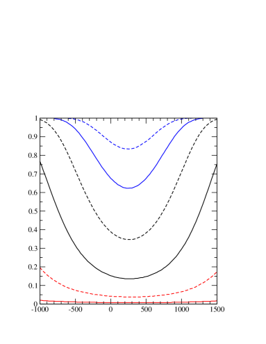
Figure 8: 2-body decay branching ratio as a function of $A_{0}$ for non vanishing $\lambda^{\prime}_{211}$ at the GUT scale and different $\tan\beta$. We assume down-type quark mixing. The other mSUGRA parameters are $M_{0}=0$ GeV, $M_{1/2}=500$ GeV, $\text{sgn}(\mu)=+1$. The solid red curve corresponds to $\tan\beta=7$.

We investigate the dependence of $\text{BR}_{2}$ on $A_{0}$ in Fig. 8, for a dominant coupling $\lambda^{\prime}_{211}$ and down-type mixing. We see a minimum at $A_{0}\approx 250\,$GeV. Here, $\text{BR}_{2}$ is reduced by up to 70% compared to $A_{0}=\pm 1\,\text{TeV}$. The minimum and the position of the minimum is dominated by the following two effects.

The right-handed stau couples to a left-handed stau (tau sneutrino) and a neutral Higgs (charged Higgs) via a trilinear scalar interaction $(\mathbf{h}_{E})_{33}$ Allanach:2003eb . The coupling $(\mathbf{h}_{E})_{33}$ has dimension one and in mSUGRA models it is equal to $A_{0}\times(\mathbf{Y}_{E})_{33}$ at the GUT scale. The RGE of the right-handed scalar tau mass, $m_{\tilde{\tau}_{R}}$, depends in the following way on $(\mathbf{h}_{E})_{33}^{2}$ Allanach:2003eb :

$$\frac{dm_{\tilde{\tau}_{R}^{2}}}{dt}=+4(\mathbf{h}_{E})_{33}^{2}+\dots\,.$$ (III.57)

This term decreases $m_{\tilde{\tau}_{R}}$ when we go from the GUT scale to the SUSY scale (II.37) due to the plus sign. The (negative) contribution of this term to $m^{2}_{\tilde{\tau}_{R}}$ is proportional to the integral of $(\mathbf{h}_{E})_{33}^{2}$ from $t_{\rm min}=\ln({M_{\rm GUT}})$ to $t_{\rm max}=\ln({M_{Z}})$. For the mSUGRA parameters given in Fig. 8, $M_{0}=0$ GeV, $M_{1/2}=500$ GeV, $\text{sgn}(\mu)=+1$, the integral of $(\mathbf{h}_{E})_{33}^{2}$ is minimal at $A_{0}\approx 180$ GeV and, therefore, $m_{\tilde{\tau}_{R}}$ is maximal. For $m_{\tilde{\tau}_{1}}=m_{\tilde{\tau}_{R}}$ this also leads to a maximum of $\Gamma_{4}/\Gamma_{2}\sim m_{\tilde{\tau}_{1}}^{6}$ and hence to a minimum of $\text{BR}_{2}$.

But the lightest stau is an admixture of the right- and left-handed stau. The off-diagonal mass matrix elements $B_{LR}$, Eq. (II.11), depend also on the value of $(\mathbf{h}_{E})_{33}$ at the SUSY scale, Eq. (II.37), through $A_{\tau}=(\mathbf{h}_{E})_{33}/(\mathbf{Y}_{E})_{33}$. For $A_{0}=180$ GeV we find $A_{\tau}\approx-110$ GeV. A negative value of $A_{\tau}$ enhances the effect of L–R-mixing which decreases $m_{\tilde{\tau}_{1}}$. Therefore, the maximum of $m_{\tilde{\tau}_{1}}$ as a function of $A_{0}$ is shifted to $A_{0}\approx 250$ GeV compared to $m_{\tilde{\tau}_{R}}$. Note however that the $A_{\tau}$ dependence of stau L–R-mixing is sub-dominant around the minimum because of $\mu\tan\beta\gg A_{\tau}$.

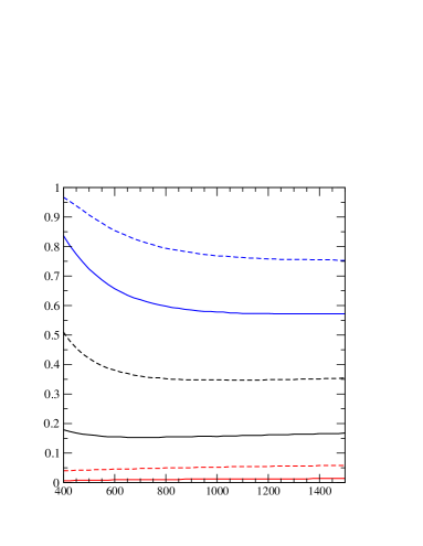
Figure 9: 2-body decay branching ratio as a function of $M_{1/2}$ for non vanishing $\lambda^{\prime}_{211}$ at the GUT scale and different $\tan\beta$. We assume quark mixing in the down sector. The other mSUGRA parameters are $M_{0}=0$ GeV, $A_{0}=600$ GeV, $\text{sgn}(\mu)=+1$. The solid red curve corresponds to $\tan\beta=7$.

Next, we study the dependence of $\text{BR}_{2}$ on the universal gaugino mass $M_{1/2}$. We show this behavior in Fig. 9, again for a dominant $\lambda^{\prime}_{211}$ and down-type mixing. The 2-body decay branching ratios approach a constant value for increasing $M_{1/2}$. Both, the squared mass of the gauginos, cf. Eq. (II.15), and the squared masses of the sfermions, cf. Eq. (II.10), depend linearly on $M_{1/2}^{2}$. Therefore,

$$\lim_{M_{1/2}\rightarrow\infty}\Gamma_{4}/\Gamma_{2}\propto\frac{m_{\tilde{\tau}_{1}}^{6}}{m_{\tilde{\chi}}^{2}m_{\tilde{f}}^{4}}=\text{constant}\,.$$ (III.58)

The dependence of $\text{BR}_{2}$ on $M_{1/2}$ for $M_{1/2}\raise 1.29167pt\hbox{$\;<$\kern-7.5pt\raise-4.73611pt\hbox{$\sim\;$}}1$ TeV is more involved, because the ratio $\Gamma_{4}/\Gamma_{2}$ depends also on the other mSUGRA parameters, mainly through the running sfermion masses, cf. Eq. (II.10). For example, we observe in Fig. 9 that the slope of $\text{BR}_{2}$ for $M_{1/2}\raise 1.29167pt\hbox{$\;<$\kern-7.5pt\raise-4.73611pt\hbox{$\sim\;$}}1\,$TeV strongly depends on $\tan\beta$. For $\tan\beta=10$, the slope is small and positive whereas for $\tan\beta\raise 1.29167pt\hbox{$\;>$\kern-7.5pt\raise-4.73611pt\hbox{$\sim\;$}}13$ the slope is negative. The magnitude of the slope also increases when we consider larger values of $\tan\beta$. This behavior is again related to the tau Yukawa coupling $(\mathbf{Y}_{E})_{33}$ and its effects on the $\tilde{\tau}_{1}$ mass described by the function $X_{\tau}$, Eq. (II.13). For large values of $M_{1/2}$, the influence of $X_{\tau}$ on the $\tilde{\tau}_{1}$ mass nearly vanishes. But as we go to smaller values of $M_{1/2}$ the (negative) contributions due to $(\mathbf{Y}_{E})_{33}$ become more and more important. For example, for $\tan\beta=22$ and $M_{1/2}=1$ TeV ($M_{1/2}=400$ GeV) the $X_{\tau}$ term reduces the mass of the right-handed stau by $3\%$ ($10\%$) compared to vanishing $(\mathbf{Y}_{E})_{33}$. This reduction of $m_{\tilde{\tau}_{1}}$ will also reduce $\Gamma_{4}/\Gamma_{2}$ resulting in an increase of $\text{BR}_{2}$. This effect is more pronounced for large $\tan\beta$ because $X_{\tau}$ is proportional to $(1+\tan^{2}\beta)$. If we neglect the effect of $(\mathbf{Y}_{E})_{33}$, the $\text{BR}_{2}$ curves in Fig. 9 all get a small positive slope.

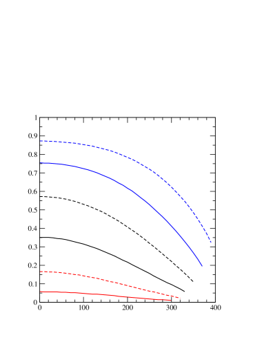
Figure 10: 2-body decay branching ratio as a function of $M_{0}$ for non vanishing $\lambda^{\prime}_{211}$ at the GUT scale and different $\tan\beta$. We assume quark mixing in the down sector. The other mSUGRA parameters are $M_{1/2}=1400$ GeV, $A_{0}=600$ GeV, $\text{sgn}(\mu)=+1$.

Finally, we show in Fig. 10 the dependence of $\text{BR}_{2}$ on the universal softbreaking scalar mass $M_{0}$. Here, we have chosen a rather large value of $M_{1/2}$, $M_{1/2}=1400$ GeV, because otherwise a $\tilde{\tau}_{1}$ LSP would exist only in a small interval of $M_{0}$.

The behavior of $\text{BR}_{2}$ can easily be understood. Increasing $M_{0}$ increases the mass of the sfermions, Eq. (II.10), but not the mass of the gauginos. Therefore, the nominator of $\Gamma_{4}/\Gamma_{2}\propto m_{\tilde{\tau}_{1}}^{6}/(m_{\tilde{\chi}}^{2}m_{\tilde{f}}^{4})$ is a polynomial of order ${\cal{O}}(M_{0}^{6})$, whereas the denominator is only a polynomial of order ${\cal{O}}(M_{0}^{4})$. Therefore, the 2-body decay branching ratios fall off for increasing $M_{0}$ as shown in Fig. 10. The lines in the Figure terminate at values of $M_{0}$ above which the $\tilde{\tau}_{1}$ is no longer the LSP.

IV Resonant single slepton production in $\tilde{\tau}_{1}$ LSP scenarios

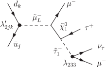
Figure 11: Example Feynman graph for single slepton production in $\tilde{\tau}_{1}$ LSP scenarios where the slepton decay proceeds via the generated $\lambda_{233}$ coupling (2-body decay mode).

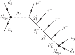
Figure 12: Example Feynman graph for single slepton production in $\tilde{\tau}_{1}$ LSP scenarios where the slepton decay proceeds via the dominant $\lambda^{\prime}_{2jk}$ coupling (4-body decay mode).

We now apply the previous discussion to resonant single slepton production in $\mathrm{B}_{3}$ mSUGRA scenarios with a $\tilde{\tau}_{1}$ LSP. Charged sleptons $\tilde{\ell}_{Li}$ and sneutrinos $\tilde{\nu}_{i}$ can be produced singly on resonance at the LHC via $q_{k}\,\bar{q}_{j}$ annihilation processes. The production cross section is proportional to $|\lambda^{\prime}_{ijk}|^{2}$ and therefore large slepton production rates are expected in scenarios with a dominant $\lambda^{\prime}_{ijk}$ coupling. The RGE generation of $\lambda_{i33}$ is important for the subsequent slepton decay in $\tilde{\tau}_{1}$ LSP scenarios. As discussed in the previous section, a non-vanishing $\lambda_{i33}$ introduces new 2-body decay channels for the $\tilde{\tau}_{1}$ LSP. The interplay of these 2-body decays and the 4-body decays via $\lambda^{\prime}_{ijk}$ determines the final state signatures. In Figs. 11 and 12, example Feynman graphs for single slepton production and the subsequent decay in $\tilde{\tau}_{1}$ LSP scenarios are shown.

It is the aim of this section to first give a general overview of the possible final states for these reactions and second to discuss the special cases $\lambda^{\prime}_{2jk}\neq 0|_{\rm GUT}$ and $\lambda^{\prime}_{3jk}\neq 0|_{\rm GUT}$ in more detail (Sects. IV.2 and IV.3).

IV.1 General Signatures

In the last section, the ratio of 2- to 4-body $\tilde{\tau}_{1}$ LSP decay rates and its dependence on various SUSY parameters has been studied. Now, we focus on single slepton production in $\tilde{\tau}_{1}$ LSP scenarios and are interested in the general decay patterns, independent of the precise SUSY parameters. We first give an overview over all possible final states and signatures which could be used as the starting point for an experimental analysis.

A (left-handed) charged slepton or sneutrino can be produced directly via $\lambda^{\prime}_{ijk}$ and has several decay modes:

$$\begin{split}{\bar{u}}_{j}\,d_{k}\rightarrow{\tilde{\ell}}_{Li}^{-}&\rightarrow\left\{\begin{array}[]{ccc}{\bar{u}}_{j}d_{k},&\\[1.29167pt] \ell^{-}_{i}\,\tilde{\chi}^{0}_{m},&\\[1.29167pt] \nu_{i}\,\tilde{\chi}^{-}_{n},&\end{array}\right.\,,\end{split}$$ (IV.59)

$$\begin{split}{\bar{d}}_{j}\,d_{k}\rightarrow{\tilde{\nu}}_{i}&\rightarrow\left\{\begin{array}[]{cc}{\bar{d}}_{j}\,d_{k},&\\[1.29167pt] \nu_{i}\,\tilde{\chi}^{0}_{m},&\\[1.29167pt] \ell^{-}_{i}\,\tilde{\chi}^{+}_{n},&\end{array}\right.\,.\end{split}$$ (IV.60)

Both can decay via the $\mathrm{B}_{3}$ coupling, which is the inverse production process. It is however suppressed by $\lvert\lambda^{\prime}_{ijk}\rvert^{2}$. If $\lambda^{\prime}_{ijk}\leq\mathcal{O}(10^{-2})$, it contributes typically at the percent level. The dominant decay channels are 2-body decays into a lepton-gaugino pair. Further 3- and more-body decays are expected to be negligible, due to phase space suppression.

In case of $j=3$, the hadronic production of a charged slepton cannot proceed via two quarks as given in Eq. (IV.59), due to the vanishing top-quark parton density inside a proton. Instead, the slepton can for example be produced via a $g\bar{d}_{k}$ initiated Compton process in association with a single top quark. Furthermore, the decay into $t\bar{d}_{k}$ may be kinematically forbidden. In this case, the slepton decays via a virtual top. The corresponding decay width is given in Appendix B. Sneutrino production for $j=3$ is possible, Eq. (IV.60), but due to the low bottom-quark density small cross sections are expected. We do not consider $j=3$ any further here and refer the reader to Bernhardt:2008mz ; Borzumati:1999th ; Accomando:2006ga ; Belyaev:2004qp for a detailed investigation of this topic.

For the following discussion, we assume that the produced slepton predominantly decays into a lepton and the lightest neutralino. This assumption is motivated by the fact that we consider $\tilde{\tau}_{1}$ LSP scenarios. In these scenarios, sleptons are light compared to gauginos and decays into heavier neutralinos or charginos will be kinematically excluded or strongly suppressed. See also the computed branching ratios in explicit SUSY models in Allanach:2006st .

The produced $\tilde{\chi}_{1}^{0}$ is not the lightest SUSY particle and will decay further into the $\tilde{\tau}_{1}$ LSP,

$$\tilde{\chi}_{1}^{0}\rightarrow\tau^{\mp}\,\tilde{\tau}_{1}^{\pm}.$$ (IV.61)

Since the neutralino is a Majorana fermion, both charge conjugated decays are possible. In most $\tilde{\tau}_{1}$ LSP scenarios this is the only possible decay mode of the neutralino. However, in some scenarios, the right-handed sleptons $\tilde{\mu}_{R}$ and $\tilde{e}_{R}$ are lighter than the $\tilde{\chi}_{1}^{0}$ and the additional channels $\tilde{\chi}_{1}^{0}\rightarrow\tilde{\ell}_{R}^{\pm}\ell^{\mp}$ are open (for $\ell=\mu,e$). The $\tilde{\ell}_{R}$ subsequently decays into the $\tilde{\tau}_{1}$ LSP, a $\tau$, and a lepton via a virtual neutralino

$$\begin{split}\tilde{\chi}_{1}^{0}\rightarrow\ell^{\mp}\,\tilde{\ell}_{R}^{\pm},\quad\tilde{\ell}_{R}^{\pm}\rightarrow\left\{\begin{array}[]{cc}\ell^{\pm}\,\tau^{\mp}\,\tilde{\tau}_{1}^{\pm}&\\[1.29167pt] \ell^{\pm}\,\tau^{\pm}\,\tilde{\tau}_{1}^{\mp}&\end{array}\right.\,.\end{split}$$ (IV.62)

These decay chains have smaller BRs than the decays in Eq. (IV.61). However, they lead to an additional lepton pair in the final state and could be, therefore, of special interest for experimental analyses.

IV.2 $\lambda^{\prime}_{2jk}\neq 0|_{\rm GUT}$, $\lambda_{233}\ll\lambda^{\prime}_{2jk}$

Let us now study more detailed the final state signatures in a scenario with $\lambda^{\prime}_{2jk}\neq 0|_{\rm GUT}$ and a generated $\lambda_{233}$ coupling which is small but non-zero at lower scales. In these scenarios, resonant single $\tilde{\mu}_{L}$ production and resonant single $\tilde{\nu}_{\mu}$ production at hadron colliders is possible,

$$\begin{split}\bar{u}_{j}\,d_{k}\rightarrow\tilde{\mu}^{-}_{L}&\rightarrow\bar{u}_{j}\,d_{k}/\mu^{-}\,\tilde{\chi}_{1}^{0},\\[8.53581pt] \bar{d}_{j}\,d_{k}\rightarrow\tilde{\nu}_{\mu}&\rightarrow\bar{d}_{j}\,d_{k}/\nu_{\mu}\,\tilde{\chi}_{1}^{0}.\end{split}$$ (IV.63)

As explained above, a small fraction of the sleptons decay via the inverse production process. Predominantly they decay into a lepton and the lightest neutralino, $\tilde{\chi}_{1}^{0}$. The decays involving heavier neutralinos or charginos are typically not accessible.

	$\bar{u}_{j}\,d_{k}\stackrel{{\scriptstyle\lambda^{\prime}}}{{\longrightarrow}}\tilde{\mu}_{L}^{-}\longrightarrow\bar{u}_{j}\,d_{k}/\mu^{-}\tilde{\chi}_{1}^{0}$
	or
	$\bar{d}_{j}\,d_{k}\stackrel{{\scriptstyle\lambda^{\prime}}}{{\longrightarrow}}\tilde{\nu}_{\mu}\longrightarrow\bar{d}_{j}\,d_{k}/\nu_{\mu}\tilde{\chi}_{1}^{0}$
	$\tilde{\chi}_{1}^{0}\rightarrow\tau^{+}\,\tilde{\tau}_{1}^{-}$	$\tilde{\chi}_{1}^{0}\rightarrow\tau^{-}\,\tilde{\tau}_{1}^{+}$
	$\Big{[}\tilde{\chi}_{1}^{0}\rightarrow\tau^{+}\,\tilde{\tau}_{1}^{-}\,\ell^{+}\ell^{-}\Big{]}$	$\Big{[}\tilde{\chi}_{1}^{0}\rightarrow\tau^{-}\,\tilde{\tau}_{1}^{+}\,\ell^{-}\ell^{+}\Big{]}$
$\lambda^{\prime}_{2jk}$	$\tilde{\tau}_{1}^{-}\rightarrow\tau^{-}\mu^{-}\,u_{j}\,\bar{d}_{k}$	$\tilde{\tau}_{1}^{+}\rightarrow\tau^{+}\mu^{+}\,\bar{u}_{j}\,d_{k}$
	$\tilde{\tau}_{1}^{-}\rightarrow\tau^{-}\mu^{+}\bar{u}_{j}d_{k}$	$\tilde{\tau}_{1}^{+}\rightarrow\tau^{+}\mu^{-}\,u_{j}\,\bar{d}_{k}$
	$\tilde{\tau}_{1}^{-}\rightarrow\tau^{-}\nu_{\mu}\,d_{j}\,\bar{d}_{k}$	$\tilde{\tau}_{1}^{+}\rightarrow\tau^{+}\bar{\nu}_{\mu}\,\bar{d}_{j}\,d_{k}$
	$\tilde{\tau}_{1}^{-}\rightarrow\tau^{-}\bar{\nu}_{\mu}\,\bar{d}_{j}\,d_{k}$	$\tilde{\tau}_{1}^{+}\rightarrow\tau^{+}\nu_{\mu}\,d_{j}\,\bar{d}_{k}$
$\lambda_{233}$	$\tilde{\tau}_{1}^{-}\rightarrow\tau^{-}\nu_{\mu}$	$\tilde{\tau}_{1}^{+}\rightarrow\tau^{+}\bar{\nu}_{\mu}$
	$\tilde{\tau}_{1}^{-}\rightarrow\tau^{-}\bar{\nu}_{\mu}$	$\tilde{\tau}_{1}^{+}\rightarrow\tau^{+}\nu_{\mu}$
	$\tilde{\tau}_{1}^{-}\rightarrow\mu^{-}\nu_{\tau}$	$\tilde{\tau}_{1}^{+}\rightarrow\mu^{+}\bar{\nu}_{\tau}$

Table 3: Slepton decay chains with all possible final states for single $\tilde{\mu}_{L}^{-}$ and single $\tilde{\nu}_{\mu}$ production via $\lambda^{\prime}_{2jk}$, respectively. The charge conjugated processes are not shown explicitly. Slepton decays into heavier neutralinos or charginos are neglected. The $\tilde{\chi}_{1}^{0}$ decays predominantly into a $\tilde{\tau}_{1}$ LSP and a $\tau$. In some scenarios, decays as in Eq. (IV.62) are possible, they are cited in brackets. Owing to the Majorana type nature of the neutralino two charge conjugated decays of the neutralino are possible (second and third column). In the first column the $\mathrm{B}_{3}$ coupling involved in the subsequent 4- or 2-body $\tilde{\tau}_{1}$ decays are given.

The difference between $\tilde{\mu}_{L}$ and $\tilde{\nu}_{\mu}$ production concerns the flavor of the initial quarks involved (which is related to different parton density functions and is thus important for the hadronic cross sections), and the nature of the lepton resulting from the slepton decay. In both processes a neutralino is produced in the predominant decay, which in turn decays into the $\tilde{\tau}_{1}$ LSP, as given in Eq. (IV.61) and Eq. (IV.62). Finally, the $\tilde{\tau}_{1}$ decays either via the dominant $\lambda^{\prime}_{2jk}$ coupling (4-body decay) or via the generated $\lambda_{233}$ coupling (2-body decay). For the 4-body decays, only the decays via virtual neutralinos have to be considered. Decay modes via virtual charginos are suppressed due to the larger mass and their weaker couplings to the predominantly right-handed $\tilde{\tau}_{1}$ LSP. The complete cascade decay chains are listed in Tab. 3.

A classification of all possible final state signatures is given in Tab. 4, for $\tilde{\mu}_{L}$ and for $\tilde{\nu}_{\mu}$ production. For completeness, we include here the direct B₃ decays via $\lambda^{\prime}_{2jk}$, which usually contribute at the percent level for couplings at the order of $\mathcal{O}(10^{-2})$. Neutrinos do not give a signal in a detector and are denoted as missing transverse energy, $\not{\!\!E}_{T}$. Final state quarks are treated as indistinguishable jets, $j$.

The 4-body decays via $\lambda^{\prime}_{2jk}$ and the 2-body decays via the inverse production process lead to two jets in the final state. In contrast, the 2-body decays via $\lambda_{233}$ are purely leptonic. Many cascade decay chains provide missing transverse energy. Furthermore, since we are considering $\tilde{\tau}_{1}$ LSP scenarios, there is always at least one $\tau$ among the final state particles. The experimentally most promising signatures are most likely those involving a large number of muons, for example like-sign dimuons and three or four final state muons. If the $\tilde{\chi}_{1}^{0}$ decays only into $\tilde{\tau}_{1}\tau$, there are two signatures including like-sign dimuons for $\tilde{\mu}_{L}$ production. For $\tilde{\nu}_{\mu}$ production, muons can be produced singly only. But if the decays Eq. (IV.62) are open, both slepton production processes allow for dimuon and trimuon production. In case of $\tilde{\mu}_{L}$ production, even four final state muons are possible. Additionally, depending on how easily taus will be identified, an analysis could be based on like-sign $\mu\tau$-pairs.

The final state signatures depend sensitively on which particle is the LSP. Compared to slepton production in the $\tilde{\chi}_{1}^{0}$ LSP scenarios Dimopoulos:1988jw ; Dimopoulos:1988fr ; Dreiner:2000vf ; Dreiner:2000qf ; Dreiner:1998gz ; Moreau:2000bs ; Deliot:2000mf ; Abazov:2002es ; Abazov:2006ii , there are three main differences here. First, for a $\tilde{\tau}_{1}$ LSP we have always one or two taus in the final state, which in $\tilde{\chi}_{1}^{0}$ LSP scenarios is only possible for smuon production if heavier neutralinos are involved in the decay chain. These heavy neutralinos then decay into the lightest neutralino and possibly taus. Second, the generation of a $\lambda$ coupling can be neglected in $\tilde{\chi}_{1}^{0}$ LSP scenarios. As argued above, $\lambda$ only allows for additional 3-body decays which are thus not phase-space enhanced compared to the 3-body decays via the dominant $\lambda^{\prime}$ coupling. As a consequence, purely leptonic final state signatures are absent in $\tilde{\chi}_{1}^{0}$ LSP scenarios. Third, due to the modified spectra in $\tilde{\chi}_{1}^{0}$ LSP scenarios, also $\tilde{\nu}_{\mu}$ production can provide like-sign dimuon events. In this case, $\tilde{\nu}_{\mu}$ can often decay into a $\mu$ and a chargino. Like-sign dimuons arise either if the chargino directly decays via $\lambda^{\prime}$ into a $\mu$ and two quarks, or if the chargino first decays into the $\tilde{\chi}_{1}^{0}$ LSP and then the $\tilde{\chi}_{1}^{0}$ LSP decays via $\lambda^{\prime}$ into a $\mu$ and two quarks.

This discussion can easily be translated to scenarios with $\lambda^{\prime}_{1jk}\neq 0$ by replacing the muons by electrons (and vice versa). Since there is typically no difference in mass between sleptons of the first and second generation, respectively, the kinematics are the same. Note however that the bounds on the $\mathrm{B}_{3}$ couplings are stronger for $\lambda^{\prime}_{1jk}$ than for $\lambda^{\prime}_{2jk}$ for example due to the non-observation of neutrinoless double beta decays.

	$\tilde{\mu}^{-}_{L}$ production
$\lambda^{\prime}_{2jk}$	$\hskip 4.30554pt\tau^{+}\,\tau^{-}$	$\mu^{-}\,\mu^{\pm}$			$jj$
	$\hskip 4.30554pt\tau^{+}\,\tau^{-}$	$\mu^{-}$		$\not{\!\!E}_{T}$	$jj$
	$[\,\tau^{+}\,\tau^{-}$	$\mu^{-}\,\mu^{-}\,\mu^{\pm}\,\mu^{+}$			$jj\,]$
	$[\,\tau^{+}\,\tau^{-}$	$\mu^{-}\,\mu^{-}\,\mu^{+}$		$\not{\!\!E}_{T}$	$jj\,]$
	$[\,\tau^{+}\,\tau^{-}$	$\mu^{-}\,\mu^{\pm}$	$e^{+}e^{-}$		$jj\,]$
	$[\,\tau^{+}\,\tau^{-}$	$\mu^{-}$	$e^{+}\,e^{-}$	$\not{\!\!E}_{T}$	$jj\,]$
$\lambda_{233}$	$\hskip 4.30554pt\tau^{\pm}$	$\mu^{-}\,\mu^{\mp}$		$\not{\!\!E}_{T}$
	$\hskip 4.30554pt\tau^{+}\,\tau^{-}$	$\mu^{-}$		$\not{\!\!E}_{T}$
	$[\,\tau^{\pm}$	$\mu^{-}\,\mu^{-}\,\mu^{\mp}\,\mu^{+}$		$\not{\!\!E}_{T}$	$\hskip 12.91663pt]$
	$[\,\tau^{+}\,\tau^{-}$	$\mu^{-}\,\mu^{-}\mu^{+}$		$\not{\!\!E}_{T}$	$\hskip 12.91663pt]$
	$[\,\tau^{\pm}$	$\mu^{-}\,\mu^{\mp}$	$e^{+}\,e^{-}$	$\not{\!\!E}_{T}$	$\hskip 12.91663pt]$
	$[\,\tau^{+}\,\tau^{-}$	$\mu^{-}$	$e^{+}\,e^{-}$	$\not{\!\!E}_{T}$	$\hskip 12.91663pt]$
inv. prod.					$jj$
	$\tilde{\nu}_{\mu}$ production
$\lambda^{\prime}_{2jk}$	$\hskip 4.30554pt\tau^{+}\,\tau^{-}$	$\mu^{\pm}$		$\not{\!\!E}_{T}$	$jj$
	$\hskip 4.30554pt\tau^{+}\,\tau^{-}$			$\not{\!\!E}_{T}$	$jj$
	$[\,\tau^{+}\,\tau^{-}$	$\mu^{-}\,\mu^{\pm}\,\mu^{+}$		$\not{\!\!E}_{T}$	$jj\,]$
	$[\,\tau^{+}\,\tau^{-}$	$\mu^{-}\,\mu^{+}$		$\not{\!\!E}_{T}$	$jj\,]$
	$[\,\tau^{+}\,\tau^{-}$	$\mu^{\pm}$	$e^{+}\,e^{-}$	$\not{\!\!E}_{T}$	$jj\,]$
	$[\,\tau^{+}\,\tau^{-}$		$e^{+}\,e^{-}$	$\not{\!\!E}_{T}$	$jj\,]$
$\lambda_{233}$	$\hskip 4.30554pt\tau^{\pm}$	$\mu^{\mp}$		$\not{\!\!E}_{T}$
	$\hskip 4.30554pt\tau^{+}\,\tau^{-}$			$\not{\!\!E}_{T}$
	$[\,\tau^{\pm}$	$\mu^{-}\,\mu^{\mp}\,\mu^{+}$		$\not{\!\!E}_{T}$	$\hskip 12.91663pt]$
	$[\,\tau^{+}\,\tau^{-}$	$\mu^{-}\,\mu^{+}$		$\not{\!\!E}_{T}$	$\hskip 12.91663pt]$
	$[\,\tau^{\pm}$	$\mu^{\mp}$	$e^{+}\,e^{-}$	$\not{\!\!E}_{T}$	$\hskip 12.91663pt]$
	$[\,\tau^{+}\,\tau^{-}$		$e^{+}\,e^{-}$	$\not{\!\!E}_{T}$	$\hskip 12.91663pt]$
inv. prod.					$jj$

Table 4: Summary of all possible final states for single slepton production via $\lambda^{\prime}_{2jk}$. Decays involving the dominant $\lambda^{\prime}_{2jk}$ coupling and involving the generated $\lambda_{233}$ coupling are listed separately, cf. Tab. 3. If kinematically allowed, the $\tilde{\chi}_{1}^{0}$ may also decay into a light-flavor lepton-slepton pair which gives rise to an additional $\mu^{+}\mu^{-}$ or $e^{+}e^{-}$ pair in the final state. The corresponding signatures are given in brackets. The decay via the inverse production process is also listed.

IV.3 $\lambda^{\prime}_{3jk}\neq 0|_{\rm GUT}$

Some additional remarks are in order for a dominant $\lambda^{\prime}_{3jk}$ $\mathrm{B}_{3}$ coupling. These couplings allow for resonant single $\tilde{\nu}_{\tau}$ production and, owing to the L-R-mixing in the stau-sector, also both resonant $\tilde{\tau}_{1}$ and $\tilde{\tau}_{2}$ production ($j\not=3$).

For $\tilde{\tau}_{1}$ production, we refer to the discussion of LSP decay modes in Sect. III.1. Here the LSP couples directly to the $\mathrm{B}_{3}$ operator and the inverse production process dominates the decay rate,

$$\bar{u}_{j}\,d_{k}\rightarrow\tilde{\tau}_{1}^{-} \rightarrow\bar{u}_{j}\,d_{k}\,.$$ (IV.64)

This decay is kinematically accessible if $j\neq 3$. For $j=3$ the stau decays via a virtual top-quark, cf. Eq. (III.53), for $m_{\tilde{\tau}_{1}}<m_{t}$. Note that $j=3$ requires associated production, e.g. $g\,d_{k}\rightarrow\tilde{\tau}\,t$, due to the absence of top quarks inside the proton Bernhardt:2008mz ; Borzumati:1999th ; Accomando:2006ga ; Belyaev:2004qp .

For $\tilde{\tau}_{2}$ and $\tilde{\nu}_{\tau}$ production, there are the following 2-body decay modes:

$$\begin{split}\bar{u}_{j}\,d_{k}\rightarrow\tilde{\tau}_{2}^{-}&\rightarrow\left\{\begin{array}[]{lll}\bar{u}_{j}\,d_{k},\\ \tau^{-}\,\tilde{\chi}_{1}^{0}\\ \tilde{\tau}_{1}^{-}\,h^{0}/Z^{0}\\ \end{array}\right.\,,\end{split}$$ (IV.65)

$$\begin{split}\bar{d}_{j}\,d_{k}\rightarrow\tilde{\nu}_{\tau}&\rightarrow\left\{\begin{array}[]{lll}\bar{d}_{j}\,d_{k},\\ \nu_{\tau}\,\tilde{\chi}_{1}^{0}\\ \tilde{\tau}_{1}^{-}\,W\\ \end{array}\right.\,.\end{split}$$ (IV.66)

The inverse production process contributes and leads to a $jj$ final state. The decay into a lepton and a neutralino often dominates for small $\tan\beta$ ($\tan\beta\raise 1.29167pt\hbox{$\;<$\kern-7.5pt\raise-4.73611pt\hbox{$\sim\;$}}10$). The neutralino decays further into the $\tilde{\tau}_{1}$ LSP which directly decays into two quarks:

$$\begin{split}\tilde{\chi}_{1}^{0}\rightarrow\,\tau^{\pm}\,&\tilde{\tau}_{1}^{\mp},\quad\tilde{\tau}_{1}^{-}\rightarrow\bar{u}_{j}\,d_{k}\,,\end{split}$$ (IV.67)

where we have included the two charge conjugated decays of the neutralino. The final states of these decay modes are $\tau^{-}\tau^{\pm}jj$, and there is the possibility of like-sign tau events. If the $\tilde{\chi}_{1}^{0}$ decay (IV.62) is kinematically allowed, we can have an additional pair of electrons or muons in the final state.

The singly produced slepton can also decay into the $\tilde{\tau}_{1}$ LSP and a SM particle, $Z^{0}$, $h^{0}$, or $W$, respectively (final states: $h^{0}/Z^{0}/W\,jj$). This decay mode is special for singly produced sleptons of the third generation because they are L-R mixed eigenstates. It can be the dominant decay mode of the $\tilde{\tau}_{2}$ and $\tilde{\nu}_{\tau}$, depending on the parameters.

The branching ratios for all $\mathrm{B}_{3}$ conserving $\tilde{\tau}_{2}$ and $\tilde{\nu}_{\tau}$ 2-body decay modes are given in Tab. 11 in Appendix B, for the SUSY parameter sets A and B.

V Single smuon production: An Explicit Numerical Example

In this section, we present explicit calculations of promising signal rates for resonant slepton production at the LHC in the $\mathrm{B}_{3}$ mSUGRA model with a $\tilde{\tau}_{1}$ LSP, focussing on parameter sets A and B, cf. Eq. (II.16). First, we consider in Sect. V.1 (exclusive) like-sign dimuon events, i.e. events with exactly two muons of the same charge in the final state. An analysis of SM and SUSY backgrounds for the like-sign dimuon signature is given in Sect. V.2. Second, in Sect. V.3, we present event rates for single smuon production leading to three or four muons in the final states, which are kinematically accessible within sets A and B.

V.1 Like-Sign Dimuon Events

Following Refs. Dreiner:2000qf ; Dreiner:2000vf , we first concentrate on events with exclusive like-sign dimuons. Here events with more than two muons are rejected. In this sense, in $\tilde{\tau}_{1}$ LSP scenarios, only single smuon production leads to exclusive like-sign dimuon pairs, cf. Tab. 4. It has been shown in Refs. Dreiner:2000qf ; Dreiner:2000vf that this selection criterion enhances the signal to background ratio considerably. In Refs. Dreiner:2000qf ; Dreiner:2000vf it was shown that using a set of cuts, the SM background rate at the LHC, $\Gamma_{B}|_{\rm SM}$, can be reduced to

$$\Gamma_{B}|_{\rm SM}=4.9\pm 1.6\;\text{events/10 fb}^{-1}.$$ (V.68)

At the same time the cut efficiency, i.e. the number of signal events which pass the cuts, lies roughly between $20\%$ and $30\%$. Note that Refs. Dreiner:2000qf ; Dreiner:2000vf assume a $\tilde{\chi}_{1}^{0}$ LSP. As we will argue in Sect. V.2, similar cuts are also applicable in $\tilde{\tau}_{1}$ LSP scenarios. For the numbers presented in this section, however, no cuts are applied and full cross sections and event rates are given.

The total cross section for like-sign dimuon events is given by the resonant $\tilde{\mu}_{L}^{+}$ or $\tilde{\mu}_{L}^{-}$ production cross section multiplied by the respective branching ratios leading to like-sign dimuon final states. Both decays via the dominant $\lambda^{\prime}_{2jk}$ coupling and a generated $\lambda_{233}$ coupling contribute. For a negatively charged smuon they are:

$$\begin{split}\bar{u}_{j}\,d_{k}\stackrel{{\scriptstyle\lambda^{\prime}}}{{\longrightarrow}}\tilde{\mu}_{L}^{-}\rightarrow\mu^{-}&\tilde{\chi}_{1}^{0},\\ &\hookrightarrow\tau^{+}\,\tilde{\tau}_{1}^{-}\\ &\qquad\quad\stackrel{{\scriptstyle\lambda^{\prime}}}{{\hookrightarrow}}\tau^{-}\mu^{-}\,u_{j}\,\bar{d}_{k}\,,\\ &\qquad\quad\stackrel{{\scriptstyle\lambda}}{{\hookrightarrow}}\nu_{\tau}\,\mu^{-}\,,\\ &\hookrightarrow\tau^{-}\,\tilde{\tau}_{1}^{+}\\ &\qquad\quad\stackrel{{\scriptstyle\lambda^{\prime}}}{{\hookrightarrow}}\tau^{+}\mu^{-}\,u_{j}\,\bar{d}_{k}\,,\end{split}$$ (V.69)

plus the analogous decay chains where the neutralino decays first into an $\tilde{e}_{R}^{\pm}$-$e^{\mp}$ pair, cf. Eq. (IV.62). The couplings depicted on the arrows indicate the employed $\mathrm{B}_{3}$ coupling. The decay chain for a positively charged smuon can be obtained by charge conjugation. However, one should keep in mind that the production cross sections for $\tilde{\mu}^{+}_{L}$ and $\tilde{\mu}^{-}_{L}$ differ at $pp$ colliders, since charge conjugated quarks (and corresponding parton densities) are involved.

The cross sections for the exclusive like-sign dimuon final states are presented in Tab. 5 for Set A and in Tab. 6 for Set B. The smuon production cross sections, $\sigma_{\rm prod.}(\tilde{\mu}_{L}^{\mp})$ (see also Tabs. 9 and 10), include NLO QCD and SUSY-QCD corrections Dreiner:2006sv , see Appendix A. For the numerical analysis, we only consider couplings $\lambda^{\prime}_{2jk}$ that involve partons of the first generation leading to large production cross sections at the LHC.

As already discussed, the $\tilde{\tau}_{1}$ LSP can either decay via $\lambda^{\prime}$ (4-body decay) or via $\lambda$ (2-body decay). A list of the respective branching ratios is given in Appendix A, Tabs. 12 and 13, for sets A and B and for several $\lambda^{\prime}_{2jk}$ couplings. Here we show the resulting cross section times branching ratio, $\sigma_{\rm prod.}\times\text{BR}_{\lambda^{\prime}}$ and $\sigma_{\rm prod.}\times\text{BR}_{\lambda}$, for like-sign dimuon events involving $\tilde{\tau}_{1}$ decays via $\lambda^{\prime}$ and $\lambda$, respectively, as described in Eq. (V.69).

				up-type mixing		down-type mixing
Set A			$\sigma_{\rm prod.}(\tilde{\mu}^{\mp}_{L})$ [fb]	$\sigma_{\rm prod.}\times\text{BR}_{\lambda^{\prime}}$	$\sigma_{\rm prod.}\times\text{BR}_{\lambda}$	$\sigma_{\rm prod.}\times\text{BR}_{\lambda^{\prime}}$	$\sigma_{\rm prod.}\times\text{BR}_{\lambda}$
		$\mu^{-}\,\mu^{-}$	61.6	11.1	0.71	9.81	2.09
$\lambda^{\prime}_{211}$	$=2\times 10^{-3}|_{\rm GUT}$	$\mu^{+}\,\mu^{+}$	108	19.4	1.25	17.2	3.66
		$\mu^{-}\,\mu^{-}$	42.0	7.84	$-$	4.51	3.88
$\lambda^{\prime}_{221}$	$=2\times 10^{-3}|_{\rm GUT}$	$\mu^{+}\,\mu^{+}$	16.2	3.03	$-$	1.74	1.50
		$\mu^{-}\,\mu^{-}$	18.6	3.46	$-$	1.99	1.71
$\lambda^{\prime}_{212}$	$=2\times 10^{-3}|_{\rm GUT}$	$\mu^{+}\,\mu^{+}$	86.0	16.1	$-$	9.23	7.94
		$\mu^{-}\,\mu^{-}$	8.80	1.67	$-$	1.32	0.40
$\lambda^{\prime}_{213}$	$=2\times 10^{-3}|_{\rm GUT}$	$\mu^{+}\,\mu^{+}$	49.8	9.43	$-$	7.43	2.24

Table 5: Cross sections for exclusive like-sign dimuon ($\mu^{-}\mu^{-}$ or $\mu^{+}\mu^{+}$) final states at the LHC within Set A. In the left column, we present the single-smuon production cross sections, $\sigma_{\text{prod.}}(\tilde{\mu}_{L}^{\mp})$, see also Tabs. 9 and 10. In the right column, we have folded in the relevant decay branching ratios, in order to obtain like-sign dimuons. All cross sections are given in fb. Where they exist, we have assumed always a cascade of 2-body decays. We consider in turn quark mixing in the up- and down-sector, when determining the dominant $\tilde{\tau}_{1}$ decay mode. The $\tilde{\tau}_{1}$ LSP can either decay via $\lambda^{\prime}$ (4-body decay) or via $\lambda$ (2-body decay), cf. Tab. 3, which leads to different like-sign dimuon cross sections, $\sigma_{\rm prod.}\times\text{BR}_{\lambda^{\prime}}$ and $\sigma_{\rm prod.}\times\text{BR}_{\lambda}$, respectively. The $\lambda^{\prime}_{2jk}$ couplings are in accordance with neutrino mass bounds Allanach:2003eb ; Markus:2008 . In case of up-type mixing, larger values of $\lambda^{\prime}_{2jk}$ for the four considered couplings are allowed by the neutrino mass bounds. The cross sections scale with $|\lambda^{\prime}|^{2}$ and the corresponding rescaling can easily be performed.

				up-type mixing		down-type mixing
Set B			$\sigma_{\rm prod.}(\tilde{\mu}^{\mp}_{L})$ [fb]	$\sigma_{\rm prod.}\times\text{BR}_{\lambda^{\prime}}$	$\sigma_{\rm prod.}\times\text{BR}_{\lambda}$	$\sigma_{\rm prod.}\times\text{BR}_{\lambda^{\prime}}$	$\sigma_{\rm prod.}\times\text{BR}_{\lambda}$
		$\mu^{-}\,\mu^{-}$	476	1.04	101	0.21	102
$\lambda^{\prime}_{211}$	$=1\times 10^{-2}|_{\rm GUT}$	$\mu^{+}\,\mu^{+}$	885	1.93	188	0.39	189
		$\mu^{-}\,\mu^{-}$	309	62.8	$-$	$-$	66.2
$\lambda^{\prime}_{221}$	$=1\times 10^{-2}|_{\rm GUT}$	$\mu^{+}\,\mu^{+}$	105	21.4	$-$	$-$	22.5
		$\mu^{-}\,\mu^{-}$	123	25.1	$-$	$-$	26.3
$\lambda^{\prime}_{212}$	$=1\times 10^{-2}|_{\rm GUT}$	$\mu^{+}\,\mu^{+}$	681	139	$-$	$-$	146
		$\mu^{-}\,\mu^{-}$	54.6	11.2	$-$	0.02	11.7
$\lambda^{\prime}_{213}$	$=1\times 10^{-2}|_{\rm GUT}$	$\mu^{+}\,\mu^{+}$	370	75.6	$-$	0.16	79.4

Table 6: Same as Tab. 5 but for single slepton production within Set B. The neutrino mass bounds are less restrictive in the case of Set B and $\lambda^{\prime}_{2jk}=0.01|_{\rm GUT}$ are considered for both up- and down-type quark mixing. All cross sections are given in fb.

The total number of exclusive like-sign dimuon events is given by the integrated luminosity multiplied by the total cross section. In Set A with up-type (down-type) quark mixing, we obtain per 10 fb^-1

$$\begin{split}&N(\mu^{-}\mu^{-}+\mu^{+}\mu^{+})/10\,\text{fb}^{-1}=\\[2.15277pt] &\Big{[}\sigma_{\rm prod.}(\tilde{\mu}^{-}_{L})+\sigma_{\rm prod.}(\tilde{\mu}^{+}_{L})\Big{]}\times\Big{[}\text{BR}_{\lambda^{\prime}}+\text{BR}_{\lambda}\Big{]}\times 10\\ &\approx\begin{cases}325\;\;(330)\\ 110\;\;(115)\\ 195\;\;(210)\\ 110\;\;(115)\end{cases}\!\!\!/10\,\text{fb}^{-1}\;\;\;\textnormal{for}\;\begin{cases}\lambda^{\prime}_{211}\\ \lambda^{\prime}_{221}\\ \lambda^{\prime}_{212}\\ \lambda^{\prime}_{213}\end{cases}\!\!\!\!=0.002\lvert_{\rm GUT}.\end{split}$$ (V.70)

Note that for up-type mixing, some larger couplings may be considered. From the neutrino mass bounds, also $\lambda^{\prime}_{211,\,221,\,212,\,213}=0.01|_{\rm GUT}$ (and even larger) are allowed. The cross sections are proportional to $|\lambda^{\prime}|^{2}$ and thus a five times larger coupling implies cross sections and event numbers multiplied by a factor of 25 compared to those of Tab. 5.

For Set B, $\lambda^{\prime}_{2jk}=0.01|_{\rm GUT}$ is allowed for both up- and down-type mixing. The numbers of like-sign dimuon events are,

$$\begin{split}&N(\mu^{-}\mu^{-}+\mu^{+}\mu^{+})/10\,\text{fb}^{-1}=\\ &\approx\begin{cases}2920\,(2920)\\ 840\;\;\,(890)\\ 1640\,(1720)\\ 870\,\;\;(910)\end{cases}\!\!\!/10\,\text{fb}^{-1}\;\;\;\textnormal{for}\;\begin{cases}\lambda^{\prime}_{211}\\ \lambda^{\prime}_{221}\\ \lambda^{\prime}_{212}\\ \lambda^{\prime}_{213}\end{cases}\!\!\!\!=0.01\lvert_{\rm GUT},\end{split}$$ (V.71)

for up-type (down-type) quark mixing, respectively.

As can be seen in Eqs. (V.70), (V.71), for each non-zero $\lambda^{\prime}$ coupling the total event numbers for up- and down-mixing are of the same order. But as Tabs. 5 and 6 show, the parts contributing to the event rate can be quite different. In case of up-type mixing and $j\neq k$, the 4-body decays via $\lambda^{\prime}$ dominate and the contributions of the 2-body decay are negligible [since the size of the necessary $\lambda$ coupling is proportional to $\big{(}\mathbf{Y}_{D}\big{)}_{jk}$]. In contrast, for down-type mixing all four considered couplings can generate a relatively large $\lambda_{233}$, cf. Fig. 2, and the 2-body decay modes contribute considerably. In Set B, where $\tan\beta$ is large and where thus the fraction of 2-body decays is especially high (see discussion of Fig. 6), reliable event numbers are only obtained if the generation of $\lambda_{233}$ is included in the theoretical framework. Moreover, a measurement of the ratio of 2-body to 4-body $\tilde{\tau}_{1}$ decays can reveal information about where the quark mixing takes place.

For $j=k$, the generation of a $\lambda$ coupling is also possible in case of up-type mixing. In Set A, the generated $\lambda_{233}$ is not large enough to allow for large 2-body decay rates. However in Set B, due to the large $\tan\beta$ value, the 2-body decays dominate over the 4-body decays. Thus, the different $\tilde{\tau}_{1}$ decay modes contain also information about $\tan\beta$.

We present in Tabs. 5 and 6 also the total hadronic cross sections for single smuon production, $\sigma_{\rm prod.}(\tilde{\mu}^{\mp}_{L})$. Within one parameter set, the cross sections vary strongly for different $\lambda^{\prime}_{2jk}$. This is of course related to corresponding required parton density functions. The largest cross section is obtained for $\lambda^{\prime}_{211}\neq 0$, i.e. for the processes $\bar{u}\,d\rightarrow\tilde{\mu}_{L}^{-}$ and $u\,\bar{d}\rightarrow\tilde{\mu}_{L}^{+}$. Smaller cross sections are obtained for $\lambda^{\prime}_{212}\neq 0$ (involving an up quark and a strange quark) and the smallest cross section for $\lambda^{\prime}_{221}\neq 0$ (charm quark and down quark) and $\lambda^{\prime}_{213}\neq 0$ (up quark together with bottom quark).

Since the LHC is a $pp$ collider, there is an asymmetry between the $\tilde{\mu}^{+}_{L}$ and $\tilde{\mu}^{-}_{L}$ production cross sections. If experimentally a distinction between $\mu^{+}\mu^{+}$ and $\mu^{-}\mu^{-}$ event rates is found, the ratio can be used to constrain the indices of the non-zero $\lambda^{\prime}_{2jk}$ coupling. For example, a non-vanishing coupling $\lambda^{\prime}_{211}$ leads to a ratio of $N(\mu^{+}\mu^{+}):N(\mu^{-}\mu^{-})\sim 2:1$ in sets A and B, whereas for non-vanishing $\lambda^{\prime}_{221}$ the ratio is $1:2.5$ in Set A and $1:3$ in Set B. The highest event rates are obtained for processes that involve the valence quarks $u$ and $d$. The charge conjugated processes, involving $\bar{u}$ or $\bar{d}$, are suppressed in comparison. Thus, a larger fraction of $\mu^{+}\mu^{+}$ events goes along with $j=1$ (where the production process is $u\,\bar{d}_{k}\rightarrow\tilde{\mu}^{+}_{L}$) and a larger fraction of $\mu^{-}\mu^{-}$ events is related to $k=1$ and $j\not=1$ (production process $\bar{u}_{j}\,d\rightarrow\tilde{\mu}^{-}_{L}$).

V.2 Discussion of Background and Cuts for Like-Sign Dimuon Final States

In this section, we discuss the background for like-sign dimuon events from the SM and from SUSY particle pair production via gauge interactions. We follow Refs. Dreiner:2000qf ; Dreiner:2000vf closely. There, single smuon production via $\lambda^{\prime}_{211}$ was investigated assuming a $\tilde{\chi}_{1}^{0}$ LSP. A detailed signal over background analysis was performed based on like-sign dimuon events. We argue that a similar or even the same set of cuts might be used to suppress the background in our case and we compare background and signal rates to determine the discovery potential of our analysis.

The main SM background sources are $t\bar{t}$ production, $b\bar{b}$ production, single top production, and gauge boson pair production, i.e. $WW$, $WZ$ and $ZZ$ production. In Refs. Dreiner:2000qf ; Dreiner:2000vf , the dominant signature from single smuon production including like-sign dimuon events is

$$\tilde{\mu}_{L}^{-}\rightarrow\mu^{-}\tilde{\chi}^{0}_{1}\rightarrow\mu^{-}(\mu^{-}u\bar{d}).$$ (V.72)

The two muons of the signal (V.72) are isolated because they stem from different decays of SUSY particles. In addition, the muons carry large momenta since they originate from the decay of (heavy) SUSY particles. The following cuts were proposed to improve the signal over SM background ratio at the LHC:

• The muon rapidity $|\eta|<2.0$, thus requiring all the leptons in the central region of the detector,

• a cut on the transverse momentum on each muon: $p_{T}|_{\mu}\geq 40$ GeV,

• an isolation cut on each of the muons,

• a cut on the transverse mass of each of the muons, 60 GeV $<M_{T}<$ 85 GeV,

• a veto on the presence of a muon with the opposite charge as the like-sign dimuons,

• a cut on the missing transverse energy, $\not{\!\!E}_{T}\leq 20\,\text{GeV}$ .

These cuts reduce the SM background to $4.9\pm 1.6$ events per 10 fb^-1 at the LHC , cf. Eq. (V.68). Among the above cuts, the isolation and $p_{T}$ cut lead to the strongest suppression of the SM background.

We now investigate the case of a $\tilde{\tau}_{1}$ LSP. If the 4-body decays (III.50) of the $\tilde{\tau}_{1}$ LSP dominate, the leading signature of resonant single smuon production including like-sign dimuon events can be written as

$$\tilde{\mu}_{L}^{-}\rightarrow\mu^{-}\tilde{\chi}^{0}_{1}\rightarrow\mu^{-}\tau^{\mp}\tilde{\tau}^{\pm}\rightarrow\mu^{-}\tau^{\mp}(\tau^{\pm}\mu^{-}u\bar{d}).$$ (V.73)

As above, the muons originate from the decay of heavy particles ($\tilde{\tau}_{1}$ and $\tilde{\mu}_{L}$), are in general well isolated, and carry large momenta. Thus, for both signals Eq. (V.72) and Eq. (V.73), the same cuts should allow to discriminate between the signal and the SM background. Furthermore, the additional pair of taus in Eq. (V.73) allows to require one or two (isolated!) taus. This might additionally improve the signal to background ratio.

If the $\tilde{\tau}_{1}$ LSP predominantly decays via 2-body decay modes, Eq. (III.51), the situation is a bit different. The like-sign dimuon signature is now

$$\tilde{\mu}_{L}^{-}\rightarrow\mu^{-}\tilde{\chi}^{0}_{1}\rightarrow\mu^{-}\tau^{+}\tilde{\tau}^{-}\rightarrow\mu^{-}\tau^{+}(\mu^{-}\nu_{\tau}).$$ (V.74)

We again have two isolated muons with large momenta and the same isolation and $p_{T}|_{\mu}$ cuts as before should be useful to suppress the SM background. But the neutrino of the $\tilde{\tau}_{1}$ decay leads to high missing transverse energy $\not{\!\!E}_{T}$ in the signal and an upper bound on $\not{\!\!E}_{T}$ is not appropriate anymore. Alternatively we propose a cut that requires a minimum missing energy, e.g. $\not{\!\!E}_{T}\geq 60$ GeV. This would also reduce the SM background where the main source of $\not{\!\!E}_{T}$ are low-energetic neutrinos from $W$ decays. Furthermore, we can again require an additional tau in the final state. Finally, one can exploit the fact that the 2-body decays lead to a pure leptonic final state and a jet veto can be applied.

In Refs. Dreiner:2000qf ; Dreiner:2000vf , the SUSY background on like-sign dimuon events is suppressed by vetoing all events with more than two jets of $p_{T}|_{\rm jet}>50$ GeV. This cut will also work if the 4-body decay mode of the $\tilde{\tau}_{1}$ LSP (III.50) dominates. The 2-body decay modes lead to purely leptonic final states and even no high-$p_{T}$ jet may be required.

We conclude that for $\tilde{\tau}_{1}$ LSP scenarios, the background for like-sign dimuon events can be suppressed similarly as it has been proposed for $\tilde{\chi}_{1}^{0}$ LSP scenarios in Dreiner:2000qf ; Dreiner:2000vf .

We thus compare our signal, as given in Eq. (V.70) and Eq. (V.71) for sets A and B respectively, to the background, assuming that cuts as discussed above reduce the SM background to less than 5 events per 10 fb^-1, cf. Eq. (V.68). For the signal efficiency, we assume $20\%$, i.e. $20\%$ of signal events pass the cuts. We neglect systematic errors, at this stage of the analysis.

For Set A a more than 5$\sigma$ excess over the SM background can be obtained for an integrated luminosity of 10 fb^-1 for all couplings given in Eq. (V.70). For Set B, a cut efficiency of $20\%$ for the signal corresponds to an excess between $100\,\sigma$ and $300\,\sigma$ for the number of like-sign muon events over the SM background! Therefore, within Set B, couplings can be tested at the LHC down to $\lambda^{\prime}_{2jk}\lvert_{\rm GUT}\sim\mathcal{O}(10^{-3})$. But a detailed Monte-Carlo based signal over background analysis remains to be done.

V.3 Final States with 3 and 4 Muons

Set A	$\sigma(--+)$	$\sigma(++-)$	$\sigma(--++)$	$\sigma(+++-)$	$\sigma(---+)$	$\sum\sigma(--\dots)$	$\sum\sigma(++\dots)$
$\lambda^{\prime}_{211}=2\times 10^{-3}|_{\rm GUT}$	9.38 (9.39)	12.9 (13.0)	5.32 (5.26)	3.39 (3.35)	1.93 (1.91)	16.6 (16.6)	21.7 (21.6)
$\lambda^{\prime}_{221}=2\times 10^{-3}|_{\rm GUT}$	5.77 (5.77)	3.84 (3.74)	1.89 (1.77)	0.53 (0.49)	1.36 (1.27)	9.02 (8.81)	6.26 (6.00)
$\lambda^{\prime}_{212}=2\times 10^{-3}|_{\rm GUT}$	4.02 (3.93)	9.05 (9.24)	3.39 (3.17)	2.79 (2.61)	0.60 (0.56)	8.01 (7.66)	15.2 (15.0)
$\lambda^{\prime}_{213}=2\times 10^{-3}|_{\rm GUT}$	2.04 (2.02)	5.14 (5.19)	1.85 (1.80)	1.57 (1.53)	0.28 (0.27)	4.17 (4.09)	8.56 (8.52)

Table 7: Cross sections for signals with three or four final state muons within parameter Set A, assuming down-type (up-type) quark mixing. Given are the cross sections as defined in Eqs. (V.75)-(V.78) and the sums for two negatively or positively charged muons, $\sum\sigma(--\dots)$ or $\sum\sigma(++\dots)$, respectively. All cross sections are given in fb.

Set B	$\sigma(--+)$	$\sigma(++-)$	$\sigma(--++)$	$\sigma(+++-)$	$\sigma(---+)$	$\sum\sigma(--\dots)$	$\sum\sigma(++\dots)$
$\lambda^{\prime}_{211}=1\times 10^{-2}|_{\rm GUT}$	20.8 (20.8)	29.1 (29.1)	13.4 (13.4)	8.73 (8.73)	4.69 (4.69)	38.9 (38.9)	51.3 (51.3)
$\lambda^{\prime}_{221}=1\times 10^{-2}|_{\rm GUT}$	11.9 (12.0)	7.77 (7.59)	4.08 (3.88)	1.04 (0.98)	3.05 (2.89)	19.1 (18.7)	12.9 (12.4)
$\lambda^{\prime}_{212}=1\times 10^{-2}|_{\rm GUT}$	8.14 (7.98)	19.5 (19.9)	7.93 (7.53)	6.72 (6.39)	1.21 (1.15)	17.3 (16.7)	34.2 (33.8)
$\lambda^{\prime}_{213}=1\times 10^{-2}|_{\rm GUT}$	3.94 (3.85)	10.4 (10.6)	4.20 (4.00)	3.66 (3.48)	0.54 (0.51)	8.68 (8.36)	18.3 (18.1)

Table 8: Same as Tab. 7 but for single slepton production within Set B. All cross sections are given in fb.

To round off our studies, we consider in this section final states with more than two muons. For example, for parameter sets A and B, the $\tilde{\chi}_{1}^{0}$ cannot only decay into a $\tilde{\tau}_{1}$-$\tau$ pair but also into a $\tilde{\mu}_{R}$-$\mu$ or $\tilde{e}_{R}$-$e$ pair. These are kinematically accessible and have non-negligible branching ratios (Set A: $7.0\%$, Set B: $2.2\%$; see Tab. 11). As we have shown in Tab. 4, these decays lead to three or even four muons of mixed signs in the final state. Each of the muons stems from the decay of a different SUSY particle. Especially the four-muon final state cannot be found at a high rate in $\tilde{\chi}_{1}^{0}$ LSP scenarios and its observation could be a hint for a $\tilde{\tau}_{1}$ LSP. Therefore, we analyze the three- and four-muon final states in this section. All necessary branching ratios and production cross sections are given in the Appendix, see Tabs. 9-13.

The four–muon events may be classified into $\mu^{-}\mu^{-}\mu^{-}\mu^{+}$, $\mu^{-}\mu^{-}\mu^{+}\mu^{+}$, and $\mu^{-}\mu^{+}\mu^{+}\mu^{+}$ signatures and we introduce the notations $\sigma(---+)$, $\sigma(--++)$, and $\sigma(+++-)$, for the respective cross sections. The four-muon final states require a long decay chain and many different decays contribute at various stages. For smuon production, summing up all contributions, the cross sections can be written in the following compact form

$$\begin{split}\sigma_{\tilde{\mu}}(---+)=&\,\sigma_{\rm prod.}(\tilde{\mu}^{-}_{L})\times\text{BR}(\tilde{\mu}^{-}_{L}\rightarrow\tilde{\chi}_{1}^{0}\,\mu^{-})\,\\ &\times\text{BR}(\tilde{\chi}_{1}^{0}\rightarrow\tilde{\mu}_{R}^{+}\,\mu^{-})\times P_{\tilde{\tau}_{1}}(1\mu)\,,\\ \sigma_{\tilde{\mu}}(+++-)=&\,\sigma_{\tilde{\mu}}(---+)\times\sigma_{\rm prod.}(\tilde{\mu}^{+}_{L})/\sigma_{\rm prod.}(\tilde{\mu}^{-}_{L})\,,\\ \sigma_{\tilde{\mu}}(--++)=&\,\sigma_{\tilde{\mu}}(---+)+\sigma_{\tilde{\mu}}(+++-),\end{split}$$ (V.75)

where $P_{\tilde{\tau}_{1}}(1\mu)=\text{BR}(\tilde{\tau}_{1}^{-}\rightarrow\mu^{-}\dots)+\text{BR}(\tilde{\tau}_{1}^{+}\rightarrow\mu^{-}\dots)$ denotes the probability of a negatively charged final state muon in a $\tilde{\tau}_{1}$ decay. The difference between $\sigma_{\tilde{\mu}}(---+)$ and $\sigma_{\tilde{\mu}}(+++-)$ stems from the different partons and parton densities involved in the production cross sections.

Smuon production can also lead to exactly three final state charged muons, $\mu^{-}\mu^{-}\mu^{+}$ or $\mu^{+}\mu^{+}\mu^{-}$. The corresponding cross sections now involve the probability $P_{\tilde{\tau}_{1}}(0\mu)$ for a $\tilde{\tau}_{1}$ decay without a final state muon,

$$\begin{split}\sigma_{\tilde{\mu}}(--+)=&\,\sigma_{\rm prod.}(\tilde{\mu}^{-}_{L})\times\text{BR}(\tilde{\mu}^{-}_{L}\rightarrow\tilde{\chi}_{1}^{0}\,\mu^{-})\\ &\times\text{BR}(\tilde{\chi}_{1}^{0}\rightarrow\tilde{\mu}_{R}^{+}\,\mu^{-})\times 2P_{\tilde{\tau}_{1}}(0\mu)\,,\\ \sigma_{\tilde{\mu}}(++-)=&\,\sigma_{\tilde{\mu}}(--+)\times\sigma_{\rm prod.}(\tilde{\mu}^{+}_{L})/\sigma_{\rm prod.}(\tilde{\mu}^{-}_{L})\,.\end{split}$$ (V.76)

There are 16 different decay chains of the $\tilde{\mu}_{L}^{-}$ leading to a $\mu^{-}\mu^{-}\mu^{+}$ final state. The factor of 2 in Eq. (V.76) is a consequence of summing over all these decay chains.

The same final state signatures (exactly three muons) can be obtained via $\tilde{\nu}_{\mu}$ production. The decay chain is similar to that of a produced smuon. The missing muon from the slepton decay is here replaced by demanding a muon in the final $\tilde{\tau}_{1}$ decay,

$$\begin{split}\sigma_{\tilde{\nu}}(--+)=&\,\left[\sigma_{\rm prod.}(\tilde{\nu}_{\mu})+\sigma_{\rm prod.}(\tilde{\nu}_{\mu}^{*})\right]\\ &\times\text{BR}(\tilde{\nu}_{\mu}\rightarrow\tilde{\chi}_{1}^{0}\,\nu_{\mu})\times\text{BR}(\tilde{\chi}_{1}^{0}\rightarrow\tilde{\mu}_{R}^{+}\,\mu^{-})\\ &\times P_{\tilde{\tau}_{1}}(1\mu)\,,\\ \sigma_{\tilde{\nu}}(++-)=&\,\sigma_{\tilde{\nu}}(--+)\,.\end{split}$$ (V.77)

The total cross sections for (exactly) three final state muons are then given by

$$\begin{split}\sigma(\mp\mp\pm)=&\sigma_{\tilde{\mu}}(\mp\mp\pm)+\sigma_{\tilde{\nu}}(\mp\mp\pm).\end{split}$$ (V.78)

Tabs. 7 and 8 give an overview over the numerical results. The same $\lambda^{\prime}$ couplings as in the previous Tabs. 5 and 6 are considered. The generation of $\lambda_{233}$ has been taken into account for the $\tilde{\tau}_{1}$ decays and the cross sections give total numbers, including both 4- and 2-body $\tilde{\tau}_{1}$ decays.

We see that the sum of three– and four-muon events is in the same order of magnitude as the results for purely like-sign dimuons. For Set A, where $\text{BR}(\tilde{\chi}_{1}^{0}\rightarrow\tilde{\mu}_{R}\,\mu)=7\%$, the event numbers are even larger. In Set B, with $\text{BR}(\tilde{\chi}_{1}^{0}\rightarrow\tilde{\mu}_{R}\,\mu)=2\%$, the total contributions are smaller by a factor of about three. Depending on the experimental goals, these channels thus give important contributions and should be included in an analysis. On the other hand, these events also suggest to use three or four final state muons as a signal for slepton production since the background is expected to be very low.

VI Conclusion

$\mathrm{B}_{3}$ interactions allow for LSP decays and thus reopen large regions in the SUSY parameter space, where the LSP is charged. We have investigated for the first time in detail the phenomenology of $\mathrm{B}_{3}$ mSUGRA models with a $\tilde{\tau}_{1}$ LSP. We have hereby assumed only one non-vanishing $\mathrm{B}_{3}$ coupling $\lambda^{\prime}_{ijk}$ at $M_{\rm GUT}$.

An essential feature of the $\mathrm{B}_{3}$ mSUGRA signatures is the decay of the $\tilde{\tau}_{1}$ LSP. Given only one $\mathrm{B}_{3}$ coupling at $M_{\rm GUT}$, we would expect either a 4-body or 2-body decay of the $\tilde{\tau}_{1}$ LSP depending on whether it couples directly to the dominant $\mathrm{B}_{3}$ operator or not. However, in $\mathrm{B}_{3}$ mSUGRA models the RGEs are highly coupled and further couplings are generated at the weak scale. These are of course suppressed relative to the dominant coupling but may lead to 2-body decays, which have larger phase space and do not involve heavy propagators.

We have here numerically investigated the generation of $\lambda_{i33}$ couplings via dominant $\lambda^{\prime}_{ijk}$ couplings. The generated couplings are typically smaller by at least two orders of magnitude; see Figs. 2 and 3. We have then performed a first detailed analysis of the parameter dependence of the $\tilde{\tau}_{1}$ LSP decay modes. It turned out that in large regions of parameter space the 2-body decay dominates over the 4-body decay, see Figs. 6-10.

In the second part of the paper, we applied our results to resonant single slepton production at the LHC, which is possible in $\mathrm{B}_{3}$ scenarios with a non-zero $\lambda^{\prime}_{ijk}$ coupling. We first studied the general decay signatures. From the experimental point of view, the final states with two like-sign or even more charged leptons are of special interest. Each event is also accompanied by at least one tau.

We further investigated numerically single smuon production for $\lambda^{\prime}_{2jk}\neq 0$ within two representative $\tilde{\tau}_{1}$ LSP scenarios, i.e. for two sets of $\mathrm{B}_{3}$ mSUGRA parameters. We include the 2-body $\tilde{\tau}_{1}$ LSP decays via the generated $\lambda_{233}$ couplings in our analysis. The cross sections for like-sign dimuon final states are given in Tab. 5 and Tab. 6 and those for final states with three or four muons in Tab. 7 and Tab. 8. For example, we found resulting cross sections for exclusive like-sign dimuon events of $\mathcal{O}(100\,\text{fb})$ for $\lambda^{\prime}_{2jk}|_{\rm GUT}=0.01$. Additional three- and four-muon events can occur with the same rate. This is a novel discovery mechanism for the LHC and should be investigated in more detail, also by the LHC experimental groups.

Appendix A Cross Sections and Branching Ratios relevant for Slepton Production and Decay

Set	$\sigma_{\rm prod.}$ [fb]				$\sigma_{\rm prod.}$ [fb]
A	$\tilde{e}_{L}^{+}/\tilde{\mu}_{L}^{+}$	$\tilde{e}_{L}^{-}/\tilde{\mu}_{L}^{-}$	$\tilde{\nu}_{e/\mu}^{*}$	$\tilde{\nu}_{e/\mu}$	$\tilde{\tau}_{2}^{+}$	$\tilde{\tau}_{2}^{-}$	$\tilde{\tau}_{1}^{+}$	$\tilde{\tau}_{1}^{-}$	$\tilde{\nu}_{\tau}^{*}$	$\tilde{\nu}_{\tau}$
$\lambda^{\prime}_{i11}=0.01\lvert_{\text{GUT}}$	$2700$	$1540$	$1860$	$1860$	$2620$	$1500$	$434$	$272$	$190$	$190$
$\lambda^{\prime}_{i22}=0.01\lvert_{\text{GUT}}$	$268$	$268$	$410$	$410$	$2600$	$2600$	$64.5$	$64.5$	$421$	$421$
$\lambda^{\prime}_{i12}=0.01\lvert_{\text{GUT}}$	$2150$	$464$	$1430$	$602$	$2090$	$451$	$360$	$103$	$1460$	$616$
$\lambda^{\prime}_{i21}=0.01\lvert_{\text{GUT}}$	$405$	$1050$	$602$	$1430$	$393$	$1020$	$91.9$	$197$	$616$	$1460$
$\lambda^{\prime}_{i13}=0.01\lvert_{\text{GUT}}$	$1240$	$220$	$788$	$292$	$1210$	$214$	$216$	$51.3$	$806$	$299$
$\lambda^{\prime}_{i23}=0.01\lvert_{\text{GUT}}$	$119$	$119$	$191$	$191$	$116$	$116$	$30.0$	$30.0$	$196$	$196$
$\lambda^{\prime}_{i31}=0.01\lvert_{\text{GUT}}$	$-$	$-$	$247$	$666$	$-$	$-$	$-$	$-$	$253$	$681$
$\lambda^{\prime}_{i32}=0.01\lvert_{\text{GUT}}$	$-$	$-$	$161$	$161$	$-$	$-$	$-$	$-$	$166$	$166$
$\lambda^{\prime}_{i33}=0.01\lvert_{\text{GUT}}$	$-$	$-$	$69.3$	$69.3$	$-$	$-$	$-$	$-$	$71.1$	$71.1$

Table 9: Complete list of hadronic cross sections for resonant single slepton/sneutrino production via $\lambda^{\prime}_{ijk}=0.01\lvert_{\rm GUT}$ at the $pp$ collider LHC ($\sqrt{S}=14$ TeV) within the parameter Set A. The cross sections include QCD and SUSY-QCD corrections at NLO Dreiner:2006sv . For $\lambda^{\prime}_{i3k}$, sleptons cannot be produced because of the vanishing top-quark density in the proton.

Set	$\sigma_{\rm prod.}$ [fb]				$\sigma_{\rm prod.}$ [fb]
B	$\tilde{e}_{L}^{+}/\tilde{\mu}_{L}^{+}$	$\tilde{e}_{L}^{-}/\tilde{\mu}_{L}^{-}$	$\tilde{\nu}_{e/\mu}^{*}$	$\tilde{\nu}_{e/\mu}$	$\tilde{\tau}_{2}^{+}$	$\tilde{\tau}_{2}^{-}$	$\tilde{\tau}_{1}^{+}$	$\tilde{\tau}_{1}^{-}$	$\tilde{\nu}_{\tau}^{*}$	$\tilde{\nu}_{\tau}$
$\lambda^{\prime}_{i11}=0.01\lvert_{\text{GUT}}$	$885$	$476$	$559$	$559$	$949$	$515$	$1168$	$750$	$657$	$657$
$\lambda^{\prime}_{i22}=0.01\lvert_{\text{GUT}}$	$67.3$	$67.3$	$102$	$102$	$74.7$	$74.7$	$192$	$192$	$124$	$124$
$\lambda^{\prime}_{i12}=0.01\lvert_{\text{GUT}}$	$681$	$123$	$414$	$155$	$735$	$136$	$976$	$301$	$490$	$187$
$\lambda^{\prime}_{i21}=0.01\lvert_{\text{GUT}}$	$105$	$309$	$155$	$414$	$117$	$337$	$269$	$548$	$187$	$490$
$\lambda^{\prime}_{i13}=0.01\lvert_{\text{GUT}}$	$370$	$54.6$	$214$	$70.2$	$401$	$60.6$	$572$	$146$	$255$	$85.4$
$\lambda^{\prime}_{i23}=0.01\lvert_{\text{GUT}}$	$28.2$	$28.2$	$44.4$	$44.4$	$31.4$	$31.4$	$87.2$	$87.2$	$54.3$	$54.3$
$\lambda^{\prime}_{i31}=0.01\lvert_{\text{GUT}}$	$-$	$-$	$60.4$	$184$	$-$	$-$	$-$	$-$	$73.5$	$219$
$\lambda^{\prime}_{i32}=0.01\lvert_{\text{GUT}}$	$-$	$-$	$38.2$	$38.2$	$-$	$-$	$-$	$-$	$46.7$	$46.7$
$\lambda^{\prime}_{i33}=0.01\lvert_{\text{GUT}}$	$-$	$-$	$14.8$	$14.8$	$-$	$-$	$-$	$-$	$18.2$	$18.2$

Table 10: Same as Tab. 9 but for parameter Set B.

In this Appendix we give the necessary cross sections and branching ratios to calculate rates of all possible decay signatures for single slepton production at the LHC, within the $\mathrm{B}_{3}$ sets A and B with a $\tilde{\tau}_{1}$ LSP, cf. Eq. (II.16).

In Tables 9 and 10, all hadronic production cross sections of resonant single sleptons within parameter Set A and Set B, respectively, are given. We consider here $\lambda^{\prime}_{ijk}=0.01|_{\text{GUT}}$, but the cross section scales with $\lvert\lambda^{\prime}_{ijk}\rvert^{2}$. The running of $\lambda^{\prime}_{ijk}$ is taken into account according to Eq. (II.31), leading to the following values at the SUSY scale $Q_{\text{susy}}$, cf. Eq. (II.37):

$$\begin{split}\text{Set A:}\quad\lambda^{\prime}_{2jk}=0.0282,\quad&\lambda^{\prime}_{3jk}=0.0282,\\ \lambda^{\prime}_{23k}=0.0258,\quad&\lambda^{\prime}_{33k}=0.0257,\\ \lambda^{\prime}_{2j3}=0.0281,\quad&\lambda^{\prime}_{3j3}=0.0280,\\ \lambda^{\prime}_{233}=0.0255,\quad&\lambda^{\prime}_{333}=0.0254;\end{split}$$ (A.79)

$$\begin{split}\text{Set B:}\quad\lambda^{\prime}_{2jk}=0.0274,\quad&\lambda^{\prime}_{3jk}=0.0271,\\ \lambda^{\prime}_{23k}=0.0249,\quad&\lambda^{\prime}_{33k}=0.0247,\\ \lambda^{\prime}_{2j3}=0.0269,\quad&\lambda^{\prime}_{3j3}=0.0266,\\ \lambda^{\prime}_{233}=0.0238,\quad&\lambda^{\prime}_{333}=0.0236,\end{split}$$ (A.80)

where $j,k=1,2$ and $Q_{\text{susy}}=893$ GeV for Set A and $Q_{\text{susy}}=1209$ GeV for Set B.

The production cross sections include NLO SUSY-QCD corrections Dreiner:2006sv . The latter depend on the trilinear quark-squark-slepton coupling, $h_{D^{k}}$, defined in Ref. Allanach:2003eb . Numerically, it is $h_{D^{k}}=-23.4$ GeV ($-21.2$ GeV) within Set A (Set B) at the SUSY scale. We incorporated the running of $h_{D^{k}}$ by using the one-loop contributions from gauge interactions Allanach:2003eb .

	$\text{BRs}\,[\%]$
	$\lambda^{\prime}_{2jk}=0.01|_{\text{GUT}}$		$\lambda^{\prime}_{3jk}=0.01|_{\text{GUT}}$
	Set A	Set B	Set A	Set B
$\tilde{\mu}_{L}^{-}\rightarrow\tilde{\chi}_{1}^{0}\,\mu^{-}$	91.1	91.3	100	100
$\tilde{\mu}_{L}^{-}\rightarrow\bar{u}_{j}\,d_{k}$	8.9	8.7	$-$	$-$
$\tilde{\nu}_{\mu}\rightarrow\tilde{\chi}_{1}^{0}\,\nu_{\mu}$	91.7	91.5	100	100
$\tilde{\nu}_{\mu}\rightarrow\bar{d}_{j}\,d_{k}$	9.3	8.4	$-$	$-$
$\tilde{\chi}_{1}^{0}\rightarrow\tilde{\tau}_{1}^{\pm}\,\tau^{\mp}$	36.0	45.7	36.0	45.7
$\tilde{\chi}_{1}^{0}\rightarrow\tilde{\mu}_{R}^{\pm}\,\mu^{\mp}$	7.0	2.2	7.0	2.2
$\tilde{\chi}_{1}^{0}\rightarrow\tilde{e}_{R}^{\pm}\,e^{\mp}$	7.0	2.1	7.0	2.1
$\tilde{\mu}_{R}^{-}\rightarrow\tilde{\tau}_{1}^{+}\,\mu^{-}\,\tau^{-}$	54.3	64.1	54.3	64.1
$\tilde{\mu}_{R}^{-}\rightarrow\tilde{\tau}_{1}^{-}\,\mu^{-}\,\tau^{+}$	45.7	35.9	45.7	35.9
$\tilde{\tau}^{-}_{2}\rightarrow\tilde{\chi}_{1}^{0}\,\tau^{-}$	58.4	14.7	55.5	14.5
$\tilde{\tau}^{-}_{2}\rightarrow\tilde{\tau}_{1}^{-}\,h^{0}$	22.5	41.8	21.4	41.2
$\tilde{\tau}^{-}_{2}\rightarrow\tilde{\tau}_{1}^{-}\,Z^{0}$	19.1	43.5	18.1	42.9
$\tilde{\tau}^{-}_{2}\rightarrow\bar{u}_{j}\,d_{k}$	$-$	$-$	5.0	1.3
$\tilde{\nu}_{\tau}\rightarrow\tilde{\chi}_{1}^{0}\,\nu_{\tau}$	62.2	13.6	58.8	13.4
$\tilde{\nu}_{\tau}\rightarrow\tilde{\tau}_{1}^{-}\,W^{+}$	37.8	86.4	35.8	85.2
$\tilde{\nu}_{\tau}\rightarrow\bar{d}_{j}\,d_{k}$	$-$	$-$	5.4	1.4

Table 11: Table of branching ratios, BRs, that are relevant for single slepton production and decays within the $\mathrm{B}_{3}$ mSUGRA scenarios Set A and Set B. Two different non-zero $\mathrm{B}_{3}$ couplings are considered, $\lambda^{\prime}_{2jk}=0.01|_{\text{GUT}}$ for columns 2 and 3 and $\lambda^{\prime}_{3jk}=0.01|_{\text{GUT}}$ for columns 4 and 5. The branching ratios for $\lambda^{\prime}_{1jk}\neq 0$ can be obtained from those for $\lambda^{\prime}_{2jk}\neq 0$ by interchanging muon and electron flavor in the first four decay channels. The branching ratios for $\tilde{e}_{L}$ ($\tilde{\nu}_{e},\,\tilde{e}_{R}$) in scenarios with $\lambda^{\prime}_{ijk}\neq 0,\,i\neq 1$ are equal to those of $\tilde{\mu}_{L}$ ($\tilde{\nu}_{\mu},\,\tilde{\mu}_{R}$) with $\lambda^{\prime}_{3jk}\neq 0$. The branching ratios for $\tilde{\tau}_{1}$ LSP decays are listed separately in Tabs. 12, 13.

Second, for the calculation of the rate for a given signature of resonant single slepton production, the branching ratios for the slepton decay and for the subsequent decay chains down to the $\tilde{\tau}_{1}$ LSP are needed. For all dominant $\lambda^{\prime}_{ijk}$ couplings these branching ratios are universal within parameter Set A and Set B, respectively, and are given in Tab. 11.

Finally, we show in Table 12 (Table 13) all branching ratios of $\tilde{\tau}_{1}$ LSP decays for different couplings $\lambda^{\prime}_{2jk}$ at the GUT scale. Branching ratios within scenarios with $\lambda^{\prime}_{1jk}\neq 0$ are analogous and can be obtained from the tables by replacing $\mu$ by $e$ in the final state signatures.

In the case of a non-vanishing $\lambda^{\prime}_{3jk}$, the $\tilde{\tau}_{1}$ LSP directly couples to the dominant $L_{3}Q_{j}\bar{D}_{k}$ operator and decays predominantly via the inverse production process, see also the discussion in Sect. III.1. For the special case of $\lambda^{\prime}_{33k}\not=0$ and $m_{\tilde{\tau}_{1}}<m_{t}$, however, the $\tilde{\tau}_{1}$ decays into a $W$ boson and two jets, cf. Eq. (III.53). The corresponding matrix element and partial width are calculated in Appendix B.

Set	$\tilde{\tau}_{1}^{-}\stackrel{{\scriptstyle\lambda}}{{\rightarrow}}\nu_{\mu}\tau^{-}$
A	[$=\tilde{\tau}_{1}^{-}\stackrel{{\scriptstyle\lambda}}{{\rightarrow}}\nu_{\tau}\mu^{-}$]		$\tilde{\tau}_{1}^{-}\stackrel{{\scriptstyle\lambda}}{{\rightarrow}}\bar{\nu}_{\mu}\tau^{-}$		$\tilde{\tau}_{1}^{-}\stackrel{{\scriptstyle\lambda^{\prime}}}{{\rightarrow}}\tau^{-}\mu^{-}u_{j}\bar{d}_{k}$		$\tilde{\tau}_{1}^{-}\stackrel{{\scriptstyle\lambda^{\prime}}}{{\rightarrow}}\tau^{-}\mu^{+}\bar{u}_{j}d_{k}$		$\tilde{\tau}_{1}^{-}\stackrel{{\scriptstyle\lambda^{\prime}}}{{\rightarrow}}\tau^{-}\nu_{\mu}d_{j}\bar{d}_{k}$		$\tilde{\tau}_{1}^{-}\stackrel{{\scriptstyle\lambda^{\prime}}}{{\rightarrow}}\tau^{-}\bar{\nu}_{\mu}\bar{d}_{j}d_{k}$
$\lambda^{\prime}_{211}$	$7.9\%$	($2.7\%$)	$0.2\%$	($0.1\%$)	$11.8\%$	($13.3\%$)	$25.3\%$	($28.5\%$)	$15.2\%$	($17.1\%$)	$31.6\%$	($35.6\%$)
$\lambda^{\prime}_{212}$	$21.5\%$	($-$)	$0.5\%$	($-$)	$7.9\%$	($14.2\%$)	$17.1\%$	($29.3\%$)	$10.2\%$	($18.1\%$)	$21.3\%$	($38.4\%$)
$\lambda^{\prime}_{213}$	$10.5\%$	($-$)	$0.2\%$	($-$)	$11.1\%$	($14.1\%$)	$23.8\%$	($30.2\%$)	$14.3\%$	($18.1\%$)	$29.6\%$	($37.6\%$)
$\lambda^{\prime}_{221}$	$21.5\%$	($-$)	$0.5\%$	($-$)	$7.9\%$	($14.2\%$)	$17.1\%$	($29.3\%$)	$10.2\%$	($18.1\%$)	$21.3\%$	($38.4\%$)
$\lambda^{\prime}_{222}$	$46.8\%$	($46.8\%$)	$1.1\%$	($1.1\%$)	$0.7\%$	($0.8\%$)	$1.6\%$	($1.6\%$)	$1.0\%$	($1.0\%$)	$2.0\%$	($2.0\%$)
$\lambda^{\prime}_{223}$	$48.2\%$	($-$)	$1.1\%$	($-$)	$0.4\%$	($14.2\%$)	$0.8\%$	($29.3\%$)	$0.5\%$	($18.2\%$)	$1.0\%$	($38.4\%$)
$\lambda^{\prime}_{231}$	$17.9\%$	($-$)	$0.4\%$	($-$)	$-$	($-$)	$-$	($-$)	$20.7\%$	($32.1\%$)	$43.0\%$	($67.9\%$)
$\lambda^{\prime}_{232}$	$48.8\%$	($-$)	$1.1\%$	($-$)	$-$	($-$)	$-$	($-$)	$0.4\%$	($32.5\%$)	$0.8\%$	($67.5\%$)
$\lambda^{\prime}_{233}$	$49.4\%$	($49.4\%$)	$1.1\%$	($1.1\%$)	$-$	($-$)	$-$	($-$)	$-$	($-$)	$-$	($-$)

Table 12: Branching ratios of the $\tilde{\tau}_{1}$ LSP for different non-zero $\lambda^{\prime}_{2jk}$ couplings at the GUT scale. The branching ratios are calculated within the mSUGRA parameter Set A for the SUSY breaking scale $Q_{\text{susy}}=893$ GeV. We assume down-type (up-type) quark mixing. Branching ratios for non-vanishing $\lambda^{\prime}_{1jk}$ are analogous, with $\mu$ replaced by $e$.

Set	$\tilde{\tau}_{1}^{-}\stackrel{{\scriptstyle\lambda}}{{\rightarrow}}\nu_{\mu}\tau^{-}$
B	[$=\tilde{\tau}_{1}^{-}\stackrel{{\scriptstyle\lambda}}{{\rightarrow}}\nu_{\tau}\mu^{-}$]		$\tilde{\tau}_{1}^{-}\stackrel{{\scriptstyle\lambda}}{{\rightarrow}}\bar{\nu}_{\mu}\tau^{-}$		$\tilde{\tau}_{1}^{-}\stackrel{{\scriptstyle\lambda^{\prime}}}{{\rightarrow}}\tau^{-}\mu^{-}u_{j}\bar{d}_{k}$		$\tilde{\tau}_{1}^{-}\stackrel{{\scriptstyle\lambda^{\prime}}}{{\rightarrow}}\tau^{-}\mu^{+}\bar{u}_{j}d_{k}$		$\tilde{\tau}_{1}^{-}\stackrel{{\scriptstyle\lambda^{\prime}}}{{\rightarrow}}\tau^{-}\nu_{\mu}d_{j}\bar{d}_{k}$		$\tilde{\tau}_{1}^{-}\stackrel{{\scriptstyle\lambda^{\prime}}}{{\rightarrow}}\tau^{-}\bar{\nu}_{\mu}\bar{d}_{j}d_{k}$
$\lambda^{\prime}_{211}$	$49.0\%$	($48.6\%$)	$1.7\%$	($1.7\%$)	$-$	($0.1\%$)	$0.1\%$	($0.4\%$)	$-$	($0.1\%$)	$0.1\%$	($0.5\%$)
$\lambda^{\prime}_{212}$	$49.1\%$	($-$)	$1.7\%$	($-$)	$-$	($5.6\%$)	$-$	($41.1\%$)	$-$	($6.3\%$)	$-$	($46.9\%$)
$\lambda^{\prime}_{213}$	$49.0\%$	($-$)	$1.7\%$	($-$)	$-$	($5.7\%$)	$0.1\%$	($41.0\%$)	$-$	($6.4\%$)	$0.1\%$	($46.9\%$)
$\lambda^{\prime}_{221}$	$49.1\%$	($-$)	$1.7\%$	($-$)	$-$	($5.6\%$)	$-$	($41.0\%$)	$-$	($6.3\%$)	$-$	($47.0\%$)
$\lambda^{\prime}_{222}$	$49.1\%$	($49.1\%$)	$1.7\%$	($1.7\%$)	$-$	($-$)	$-$	($-$)	$-$	($-$)	$-$	($-$)
$\lambda^{\prime}_{223}$	$49.1\%$	($-$)	$1.7\%$	($-$)	$-$	($5.7\%$)	$-$	($41.0\%$)	$-$	($6.4\%$)	$-$	($47.0\%$)
$\lambda^{\prime}_{231}$	$49.1\%$	($-$)	$1.7\%$	($-$)	$-$	($-$)	$-$	($-$)	$-$	($12.0\%$)	$0.1\%$	($88.0\%$)
$\lambda^{\prime}_{232}$	$49.1\%$	($-$)	$1.7\%$	($-$)	$-$	($-$)	$-$	($-$)	$-$	($12.0\%$)	$-$	($88.0\%$)
$\lambda^{\prime}_{233}$	$49.1\%$	($49.1\%$)	$1.7\%$	($1.7\%$)	$-$	($-$)	$-$	($-$)	$-$	($-$)	$-$	($-$)

Table 13: Branching ratios of the $\tilde{\tau}_{1}$ LSP for different non-zero $\lambda^{\prime}_{2jk}$ couplings at the GUT scale. The branching ratios are calculated within the mSUGRA parameter Set B for the SUSY breaking scale $Q_{\text{susy}}=1209$ GeV. We assume down-type (up-type) quark mixing. Branching ratios for non-vanishing $\lambda^{\prime}_{1jk}$ are analogous, with $\mu$ replaced by $e$.

Appendix B The $\mathrm{B}_{3}$ slepton decay $\tilde{\ell}^{-}_{i}\rightarrow W^{-}\bar{b}d_{k}$

A non-vanishing $L_{i}Q_{3}\bar{D}_{k}$ operator allows for slepton decay into a top quark $t$ and a down-type quark $d_{k}$ of generation $k$,

$$\tilde{\ell}_{i}^{-}\rightarrow\bar{t}d_{k}\,.$$ (B.81)

However, this decay mode is kinematically only allowed if $m_{\tilde{\ell}_{i}}>m_{t}+m_{d_{k}}$. For $m_{\tilde{\ell}_{i}}<m_{t}+m_{d_{k}}$, the slepton decays via a virtual top quark,

$$\tilde{\ell}_{i}^{-}\rightarrow W^{-}\bar{b}d_{k}.$$ (B.82)

This 3-body decay has not been considered in the literature yet and is not implemented in the R-parity violating version of Herwig, either. We complete the picture by calculating the 3-body decay (B.82) in the following.

The relevant parts of the supersymmetric Lagrangian are Richardson:2000nt

$$\begin{split}\mathcal{L}_{L_{i}Q_{3}\bar{D}_{k}}&=\lambda^{\prime}_{i3k}L_{1\beta}\tilde{\ell}_{i\beta}^{-}\,\bar{d}_{k}\,P_{L}\,t+h.c.\;,\\ \mathcal{L}_{bWt}&=-\frac{g}{\sqrt{2}}\,W_{\mu}^{+}\,\bar{t}\,\gamma^{\mu}\,P_{L}\,b+h.c.\;,\end{split}$$ (B.83)

where $L_{\alpha\beta}$ is the slepton mixing matrix, $\alpha$ the left/right eigenstate, and $\beta$ the mass eigenstate. From Eq. (B.83), the squared matrix element (summed over final state polarizations and colors) can be derived,

$$\begin{split}\Big{\lvert}\overline{\mathcal{M}}&\big{(}\tilde{\ell}_{i\beta}^{-}\rightarrow W^{-}\bar{b}d_{k}\big{)}\Big{\rvert}^{2}=\frac{3}{2}\frac{\lambda^{{}^{\prime}2}_{i3k}L_{1\beta}^{2}g^{2}}{[(W+b)^{2}-m_{t}^{2}]^{2}+m_{t}^{2}\Gamma_{t}^{2}}\\ &\times\Bigg{\{}2(d_{k}\!\cdot\!b)\left[m_{b}^{2}-m_{W}^{2}+4(W\!\cdot\!b)+\frac{4(W\!\cdot\!b)^{2}}{m_{W}^{2}}\right]\,\\ &\quad+4(d_{k}\!\cdot\!W)\left[m_{b}^{2}+2(W\!\cdot\!b)-m_{b}^{2}\,\frac{(W\!\cdot\!b)}{m_{W}^{2}}\right]\Bigg{\}}.\end{split}$$ (B.84)

We denote the particle four-momenta by the particle letter, and $m_{t}$, $m_{b}$, and $m_{W}$, are the top, bottom and $W$ mass, respectively. $\Gamma_{t}$ is the total width of the top quark.

From the squared matrix element (B.84) we obtain easily the partial width for the 3-body decay (B.82), see e.g. Richardson:2000nt . We show in Fig. 13 the partial width $\Gamma(\tilde{e}_{L}\rightarrow W^{-}\bar{b}d)$ as a function of the left-handed selectron mass $m_{\tilde{e}_{L}}$. Here we take $\lambda^{\prime}_{131}=0.01$ and $L_{11}=1$, in Eq. (B.84).

In comparison to the 3-body decay (B.82), the possible 4-body decays via $\lambda^{\prime}_{i3k}$ are negligible. For example for the parameter Set B with non-vanishing $\lambda^{\prime}_{331}$, the branching ratio of the 3-body $\tilde{\tau}_{1}$ LSP decay (B.82) is larger by five orders of magnitude than the branching ratio of the 4-body $\tilde{\tau}_{1}$ LSP decays.

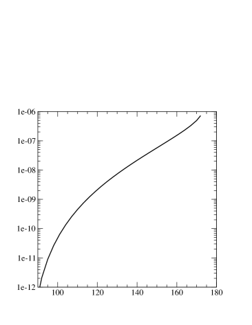
Figure 13: Partial width in GeV for the 3-body decay $\tilde{e}_{L}\rightarrow W^{-}\bar{b}d$ as a function of the selectron mass $m_{\tilde{e}_{L}}$. We take $\lambda^{\prime}_{131}=0.01$ and $L_{11}=1$, in Eq. (B.84).

References

- (1) J. Wess and B. Zumino, Nucl. Phys. B70, 39 (1974).
- (2) M. Drees, (1996), hep-ph/9611409.
- (3) H. P. Nilles, Phys. Rept. 110, 1 (1984).
- (4) S. P. Martin, (1997), hep-ph/9709356.
- (5) S. L. Glashow, Nucl. Phys. 22, 579 (1961).
- (6) S. Weinberg, Phys. Rev. Lett. 19, 1264 (1967).
- (7) [ATLAS Collab.], CERN-LHCC-94-43.
- (8) [CMS Collab.], CERN-LHCC-96-45.
- (9) B. C. Allanach, M. A. Bernhardt, H. K. Dreiner, C. H. Kom, and P. Richardson, Phys. Rev. D75, 035002 (2007), hep-ph/0609263.
- (10) B. C. Allanach, A. Dedes, and H. K. Dreiner, Phys. Rev. D69, 115002 (2004), hep-ph/0309196.
- (11) L. E. Ibáñez and G. G. Ross, Phys. Lett. B260, 291 (1991).
- (12) L. E. Ibáñez and G. G. Ross, Nucl. Phys. B368, 3 (1992).
- (13) Y. Grossman and H. E. Haber, Phys. Rev. D59, 093008 (1999), hep-ph/9810536.
- (14) H. Dreiner, C. Luhn, and M. Thormeier, Phys. Rev. D73, 075007 (2006), hep-ph/0512163.
- (15) H. K. Dreiner, C. Luhn, H. Murayama, and M. Thormeier, Nucl. Phys. B774, 127 (2007), hep-ph/0610026.
- (16) N. Sakai and T. Yanagida, Nucl. Phys. B197, 533 (1982).
- (17) S. Weinberg, Phys. Rev. D26, 287 (1982).
- (18) B. C. Allanach, A. Dedes, and H. K. Dreiner, Phys. Rev. D60, 075014 (1999), hep-ph/9906209.
- (19) A. Y. Smirnov and F. Vissani, Phys. Lett. B380, 317 (1996), hep-ph/9601387.
- (20) G. Bhattacharyya and P. B. Pal, Phys. Rev. D59, 097701 (1999), hep-ph/9809493.
- (21) R. Barbier et al., Phys. Rept. 420, 1 (2005), hep-ph/0406039.
- (22) Super-Kamiokande, M. Shiozawa et al., Phys. Rev. Lett. 81, 3319 (1998), hep-ex/9806014.
- (23) S. Dimopoulos, S. Raby, and F. Wilczek, Phys. Lett. B112, 133 (1982).
- (24) H.-S. Lee, K. T. Matchev, and T. T. Wang, Phys. Rev. D77, 015016 (2008), arXiv:0709.0763 [hep-ph].
- (25) H.-S. Lee, C. Luhn, and K. T. Matchev, JHEP 07, 065 (2008), arXiv:0712.3505 [hep-ph].
- (26) H.-S. Lee, Phys. Lett. B663, 255 (2008), arXiv:0802.0506 [hep-ph].
- (27) H. K. Dreiner, (1997), hep-ph/9707435.
- (28) H. Dreiner and G. G. Ross, Nucl. Phys. B365, 597 (1991).
- (29) R parity Working Group, B. Allanach et al., (1999), hep-ph/9906224.
- (30) S. P. Martin and M. T. Vaughn, Phys. Rev. D50, 2282 (1994), hep-ph/9311340.
- (31) B. C. Allanach, A. Dedes, and H. K. Dreiner, Phys. Rev. D60, 056002 (1999), hep-ph/9902251.
- (32) L. J. Hall and M. Suzuki, Nucl. Phys. B231, 419 (1984).
- (33) R. Hempfling, Nucl. Phys. B478, 3 (1996), hep-ph/9511288.
- (34) F. Borzumati, Y. Grossman, E. Nardi, and Y. Nir, Phys. Lett. B384, 123 (1996), hep-ph/9606251.
- (35) M. Hirsch, M. A. Diaz, W. Porod, J. C. Romao, and J. W. F. Valle, Phys. Rev. D62, 113008 (2000), hep-ph/0004115.
- (36) B. C. Allanach and C. H. Kom, JHEP 04, 081 (2008), arXiv:0712.0852 [hep-ph].
- (37) H. K. Dreiner, J. Soo Kim, and M. Thormeier, (2007), arXiv:0711.4315 [hep-ph].
- (38) J. R. Ellis, J. S. Hagelin, D. V. Nanopoulos, K. A. Olive, and M. Srednicki, Nucl. Phys. B238, 453 (1984).
- (39) A. H. Chamseddine, R. Arnowitt, and P. Nath, Phys. Rev. Lett. 49, 970 (1982).
- (40) R. Barbieri, S. Ferrara, and C. A. Savoy, Phys. Lett. B119, 343 (1982).
- (41) L. J. Hall, J. D. Lykken, and S. Weinberg, Phys. Rev. D27, 2359 (1983).
- (42) S. K. Soni and H. A. Weldon, Phys. Lett. B126, 215 (1983).
- (43) L. E. Ibanez and G. G. Ross, Phys. Lett. B110, 215 (1982).
- (44) L. E. Ibanez, C. Lopez, and C. Munoz, Nucl. Phys. B256, 218 (1985).
- (45) A. G. Akeroyd, M. A. Diaz, J. Ferrandis, M. A. Garcia-Jareno, and J. W. F. Valle, Nucl. Phys. B529, 3 (1998), hep-ph/9707395.
- (46) A. de Gouvea, A. Friedland, and H. Murayama, Phys. Rev. D59, 095008 (1999), hep-ph/9803481.
- (47) A. G. Akeroyd, C. Liu, and J.-H. Song, Phys. Rev. D65, 015008 (2002), hep-ph/0107218.
- (48) A. Bartl, M. Hirsch, T. Kernreiter, W. Porod, and J. W. F. Valle, JHEP 11, 005 (2003), hep-ph/0306071.
- (49) B. C. Allanach et al., (2007), arXiv:0710.2034 [hep-ph].
- (50) M. A. Bernhardt, H. K. Dreiner, S. Grab, and P. Richardson, Phys. Rev. D78, 015016 (2008), 0802.1482.
- (51) Kom, C. H., Cambridge, Ph.D. Thesis.
- (52) H. K. Dreiner, P. Richardson, and M. H. Seymour, Phys. Rev. D63, 055008 (2001), hep-ph/0007228.
- (53) H. K. Dreiner, P. Richardson, and M. H. Seymour, (2000), hep-ph/0001224.
- (54) H. K. Dreiner, P. Richardson, and M. H. Seymour, (1998), hep-ph/9903419.
- (55) G. Moreau, E. Perez, and G. Polesello, Nucl. Phys. B604, 3 (2001), hep-ph/0003012.
- (56) F. Deliot, G. Moreau, and C. Royon, Eur. Phys. J. C19, 155 (2001), hep-ph/0007288.
- (57) M. Chemtob, Prog. Part. Nucl. Phys. 54, 71 (2005), hep-ph/0406029.
- (58) H. K. Dreiner, M. Krämer, and B. O’Leary, Phys. Rev. D75, 114016 (2007), hep-ph/0612278.
- (59) K. Agashe and M. Graesser, Phys. Rev. D54, 4445 (1996), hep-ph/9510439.
- (60) S. Dimopoulos and L. J. Hall, Phys. Lett. B207, 210 (1988).
- (61) S. Dimopoulos, R. Esmailzadeh, L. J. Hall, and G. D. Starkman, Phys. Rev. D41, 2099 (1990).
- (62) B. C. Allanach, M. Guchait, and K. Sridhar, Phys. Lett. B586, 373 (2004), hep-ph/0311254.
- (63) D0, V. M. Abazov et al., Phys. Rev. Lett. 89, 261801 (2002), hep-ex/0207100.
- (64) D0, V. M. Abazov et al., Phys. Rev. Lett. 97, 111801 (2006), hep-ex/0605010.
- (65) D. Choudhury, S. Majhi, and V. Ravindran, Nucl. Phys. B660, 343 (2003), hep-ph/0207247.
- (66) L. L. Yang, C. S. Li, J. J. Liu, and Q. Li, Phys. Rev. D72, 074026 (2005), hep-ph/0507331.
- (67) H. K. Dreiner, S. Grab, M. Krämer, and M. K. Trenkel, Phys. Rev. D75, 035003 (2007), hep-ph/0611195.
- (68) Y.-Q. Chen, T. Han, and Z.-G. Si, JHEP 05, 068 (2007), hep-ph/0612076.
- (69) F. Borzumati, J.-L. Kneur, and N. Polonsky, Phys. Rev. D60, 115011 (1999), hep-ph/9905443.
- (70) E. Accomando et al., (2006), hep-ph/0608079.
- (71) A. Belyaev, M.-H. Genest, C. Leroy, and R. R. Mehdiyev, JHEP 09, 012 (2004), hep-ph/0401065.
- (72) M. Drees and S. P. Martin, (1995), hep-ph/9504324.
- (73) J. F. Gunion and H. E. Haber, Nucl. Phys. B272, 1 (1986).
- (74) CDF, T. Aaltonen et al., Phys. Rev. Lett. 100, 101802 (2008), 0712.1708.
- (75) Heavy Flavor Averaging Group (HFAG), E. Barberio et al., (2007), arXiv:0704.3575 [hep-ph].
- (76) Muon G-2, G. W. Bennett et al., Phys. Rev. D73, 072003 (2006), hep-ex/0602035.
- (77) J. P. Miller, E. de Rafael, and B. L. Roberts, Rept. Prog. Phys. 70, 795 (2007), hep-ph/0703049.
- (78) D. Stöckinger, (2007), arXiv:0710.2429 [hep-ph].
- (79) LEP Working Group for Higgs boson searches, R. Barate et al., Phys. Lett. B565, 61 (2003), hep-ex/0306033.
- (80) J. R. Ellis, G. Gelmini, C. Jarlskog, G. G. Ross, and J. W. F. Valle, Phys. Lett. B150, 142 (1985).
- (81) B. de Carlos and P. L. White, Phys. Rev. D54, 3427 (1996), hep-ph/9602381.
- (82) E. Nardi, Phys. Rev. D55, 5772 (1997), hep-ph/9610540.
- (83) WMAP, D. N. Spergel et al., Astrophys. J. Suppl. 148, 175 (2003), astro-ph/0302209.
- (84) M. Colless et al., (2003), astro-ph/0306581.
- (85) B. C. Allanach et al., Eur. Phys. J. C25, 113 (2002), hep-ph/0202233.
- (86) S. Kraml, http://cern.ch/kraml/comparison/.
- (87) B. C. Allanach, S. Kraml, and W. Porod, JHEP 03, 016 (2003), hep-ph/0302102.
- (88) G. Belanger, S. Kraml, and A. Pukhov, Phys. Rev. D72, 015003 (2005), hep-ph/0502079.
- (89) B. C. Allanach, Comput. Phys. Commun. 143, 305 (2002), hep-ph/0104145.
- (90) V. D. Barger, G. F. Giudice, and T. Han, Phys. Rev. D40, 2987 (1989).
- (91) W. H. Press et al., editors, Numerical Recipes in C++ (Cambridge University Press, 2002, Second Edition).
- (92) B. C. Allanach and M. A. Bernhardt, unpublished.
- (93) J. Butterworth and H. K. Dreiner, Nucl. Phys. B397, 3 (1993), hep-ph/9211204.
- (94) H. K. Dreiner and P. Morawitz, Nucl. Phys. B428, 31 (1994), hep-ph/9405253.
- (95) E. A. Baltz and P. Gondolo, Phys. Rev. D57, 2969 (1998), hep-ph/9709445.
- (96) P. Richardson, (2000), hep-ph/0101105.
- (97) F. E. Paige, S. D. Protopopescu, H. Baer, and X. Tata, (2003), hep-ph/0312045.
- (98) G. Corcella et al., JHEP 01, 010 (2001), hep-ph/0011363.
- (99) G. Corcella et al., (2002), hep-ph/0210213.
- (100) S. Moretti, K. Odagiri, P. Richardson, M. H. Seymour, and B. R. Webber, JHEP 04, 028 (2002), hep-ph/0204123.