Detecting quantum-coherent nanomechanical oscillations using the current-noise spectrum of a double quantum dot

Abstract

We consider a nanomechanical resonator coupled to a double quantum dot. We demonstrate how the finite-frequency current-noise spectrum through the double quantum dot can be used to distinguish classical and quantum behavior in the nearby nano-electromechanical resonator. We also show how the full frequency current-noise spectrum gives important information on the combined double quantum dot-resonator energy spectrum. Finally, we point out regimes where the quantum state of the resonator becomes squeezed, and also examine the cross-correlated electron-phonon current-noise.

I Introduction

The transduction of mechanical motion of resonators and cantilevers Craighead (2000); Cho (2003); Roukes and Schwab (2005); Treutlein et al. (2007); Wei et al. (2006); Blencowe (2005) has become increasingly important with the observation of motion on the nanometer-scale. In particular, when the ground state energy of the resonant mode of the mechanical system becomes larger than the thermal background temperature, a quantized state involving millions of molecules would materialize. As nanoelectromechanical systems (NEMS) reach this regime it becomes increasingly feasible, and desirable, to transduce their motion by coupling it to a quantum degree of freedom, like spinLambert et al. (2008), chargeRodrigues et al. (2007), or flux. However, the challenge of finding an appropriate measuring apparatus, one whose back-action would not destroy the fragile quantum state, has not been overcome, even if such devices could be cooled below the quantum limit Naik et al. (2006); Ouyang et al. (2008).

Here we propose using a quantized two-level ‘mesoscopic transport’ degree of freedom, or ‘transport qubit’, as a transducer of quanta exchange, and to identify signatures of quantum coherent coupled phenomena between the mechanical resonator and the transport qubit. If successfully observed, this would validate the existence of a quantized mechanical state. Here we focus on a capacitively-coupled double quantum dot realization for the transport qubit. However, our analysis applies to several other possible devices, such as superconducting single-electron transistors (SSET) Naik et al. (2006) and suspended double quantum dots Weig et al. (2004), which will be described later.

I.1 Probing mesoscopic transport

It is important to note that the types of experimental measurement that can be made on mesoscopic transport systems are limited; we can measure the average rate of particles leaving the system (current), the correlation between these currents at long times (the zero-frequency noise), and the full Fourier transform of these correlations (full frequency noise). Over the last few years, the zero-frequency noise has been used with great success to experimentally verify coherent quantum behavior (see, e.g., Ref. [Kieszlich et al., 2007]), and may in the future serve as an entanglement measure Lambert et al. (2007), and perhaps even aid in realizing a solid state test of Bell’s inequalities Beenakker et al. (2003). The full frequency noise spectrum, often more difficult to measure in practice, is appealing because it contains information about the full dynamics of the system: it reveals both coherent dynamics stemming from the system Hamiltonian $H$, and incoherent dynamics from the environment. This makes it a powerful tool for probing solid-state quantum systems.

I.2 Summary of our results

Our main result here is that we show how the coupled quantum coherent behavior, e.g., Rabi oscillations, and the low-energy part of the coupled double quantum dot-resonator spectrum, can be observed as resonances in the full frequency current noise spectrum. We also analyze the effects of temperature and decoherence on this signal, and show how the transition to the classical regime can be monitored using our approach.

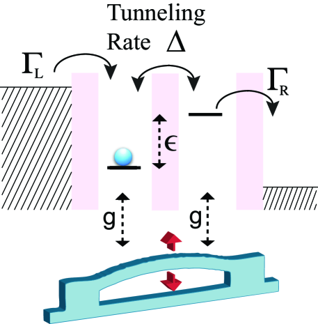
Figure 1: (Color online) Schematic diagram of a double quantum dot transport qubit (pink) coupled to a mechanical resonator (in blue). We assume a capacitive coupling $g$ between the position of the resonator and the electron charge state of the electron in the dot. The double quantum dot is attached to two electron reservoirs in the Coulomb blockade regime, with tunneling rates $\Gamma_{L}$ and $\Gamma_{R}$. There is a coherent tunneling rate $\Delta$ between the two charge states, and a tunable energy gap $\epsilon$. We assume that the mechanical resonator is already cooled to near the quantum limit Naik et al. (2006); Ouyang et al. (2008). The parameter $g$ is the coupling strength between the double quantum dot and the mechanical resonator, whose fundamental frequency is $\omega_{b}$. In the schematic diagram, the placement of the components is purely illustrative. Our model is also applicable to circuit QED systems, where coherent energy exchange between a resonator and a two-level system has recently been observed (see, e.g., Ref. [Deppe et al., 2008]).

We now proceed as follows: we first define a general model for a transport ‘qubit’ coupled to the quantized fundamental mechanical mode of a nano-electromechanical resonator. This is a well-studied model in various forms, and has been used to illustrate, e.g., boson steering and micromaser effects Brandes and Lambert (2003); Rodrigues et al. (2007); Bennett and Clerk (2006). Following this, we explain why current-noise measurements can contain signatures of quantum coherent behavior. We illustrate this with results from our master equation model for two different parameter regimes. We also identify signatures of quantum state squeezing Xue et al. (2007) of the resonator, and we calculate the correlation between tunneling events in the transport qubit and phonons leaving the mechanical resonator. Finally, we discuss other possible experimental realizations, such as suspended double quantum dots Brandes and Lambert (2003); Weig et al. (2004); Brandes (2005), spin states coupled to a magnetized resonator Lambert et al. (2008), and capacitively-coupled superconducting single electron transistors Naik et al. (2006).

II Model: Transport qubit coupled to a mechanical mode

The basic Hamiltonian for a ‘transport qubit’ coupled to a quantized mechanical resonator is as follows,

$$H=\epsilon\sigma_{z}+\Delta\sigma_{x}+g\sigma_{z}(a+a^{\dagger})+\omega_{b}a^{\dagger}a.$$ (1)

Here $\omega_{b}$ is the fundamental frequency of the resonator, $\epsilon$ is the energy gap, or splitting, of the transport qubit states, and $\Delta$ is the coherent tunneling rate between the two qubit states. The bosonic operators $a,a^{\dagger}$ destroy and create excitations in the resonator. The quasi-spin basis describes the two possible states in our transport qubit, and we assume that the transport process enters and leaves through the eigenstates of $\sigma_{z}$. For example, for our case of a double quantum dot in the Coulomb blockade regime, $\sigma_{z}=|L\rangle\langle L|-|R\rangle\langle R|$, where $L$ and $R$ represent an excess electron (N+1 total electrons) in the left or right dot, and the state $|0\rangle$ represents the empty state (N total electrons). Note that the excess electron in the double dot is well separated in energy from the other electrons due to Coulomb blockade. Alternatively, the superconducting single-electron transistor can be defined by $\sigma_{z}=|2\rangle\langle 2|-|0\rangle\langle 0|$, representing the superposition of charge states on the island. Even though superconducting single-electron transistors are three terminal devices, in certain regimes the model is equivalent to a double quantum dot Aguado and Brandes (2004) (see below). The spin-blockade case would involve a direct coupling, via the magnetization of the resonator Lambert et al. (2008), to the electron spin $\sigma_{z}=|\uparrow\rangle\langle\uparrow|-|\downarrow\rangle\langle\downarrow|$. Hereafter we retain the double quantum dot basis, $\{|L\rangle,|R\rangle\}$.

II.1 Master Equation

Transport, in all these cases, is in non-equilibrium (left to right), with a large bias applied to the device, and the current measurement monitors the electrons/particles leaving the device into the right lead/reservoir (here we neglect displacement-current contributions). The full equation of motion (master equation) for this system is described by a super-operator Liouvillian $L$ that defines the transport of particles through the “qubit” (under the Born-Markov approximation), bath damping and temperature terms for the resonator,

$$\frac{d}{dt}\rho(t) = L[\rho(t)]=-i[H,\rho(t)]+L_{0}[\rho(t)]$$ (2)

$$L_{0}[\rho(t)] = -\frac{\Gamma_{L}}{2}\left[s_{L}s_{L}^{\dagger}\rho(t)-2s_{L}^{\dagger}\rho(t)s_{L}+\rho(t)s_{L}s_{L}^{\dagger}\right]$$

$$- \frac{\Gamma_{R}}{2}\left[s_{R}^{\dagger}s_{R}\rho(t)-2s_{R}\rho(t)s_{R}^{\dagger}+\rho(t)s_{R}^{\dagger}s_{R}\right]$$

$$+ \frac{\gamma_{b}}{2}\left[-a^{\dagger}a\rho+2a\rho a^{\dagger}-\rho a^{\dagger}a\right]$$

$$+ \bar{n}\gamma_{b}\left[-a^{\dagger}a\rho+a\rho a^{\dagger}+a^{\dagger}\rho a-\rho a^{\dagger}a\right]$$

where

$$s_{L}=|0\rangle\langle L|,\,\,\,\,\,\,s_{L}^{\dagger}=|L\rangle\langle 0|,$$ (3)

$$s_{R}=|0\rangle\langle R|,\,\,\,\,\,\,s_{R}^{\dagger}=|R\rangle\langle 0|,$$ (4)

$$\bar{n}=e^{-\hbar\omega_{b}/kT}/(1-e^{-\hbar\omega_{b}/kT}),$$ (5)

$\Gamma_{L}$ and $\Gamma_{R}$ are the left/right tunneling rates, $\gamma_{b}$ is the decay rate of vibrational quanta into the resonator thermal bath, and $T$ is the temperature of the resonator thermal bath (hereafter we set $k=\hbar=1$). $\rho(t)$ is the density matrix describing the state of the resonator and the qubit.

II.2 Current-noise power

We derive the counting statistics of Eq. [2] using a generating-function approach (Appendix A). Using these equations we can calculate the current-noise power Blanter and Buttiker (2000)

$$S(\omega)_{i,j} \equiv \int_{-\infty}^{\infty}d\tau e^{i\omega\tau}\left[\langle\delta{I_{i}(t+\tau)},\delta{I_{j}(t)}\rangle\right]_{t\rightarrow\infty}$$ (6)

where $\delta I_{i}(t)$ are the current fluctuations, and $t\rightarrow\infty$ implies the fluctuations are around the steady-state expectation values. This formalism describes:

(i) particle transport through our effective ‘qubit’ ($i=j=e$, electron or particle current),

(ii) the statistics of bunching ‘vibrational phonons’ lost to the background thermal bath of the resonator ($i=j=b$, where $I_{b}$ is an effective ‘bosonic’ current),

(iii) correlations between electron and phonon events ($i\neq j$, $i=e$, $j=b$).

The electron current is defined by the operator

$$\hat{I}_{e}=\Gamma_{R}\;s_{R}\;\rho(t)\;s_{R}^{\dagger}.$$ (7)

Similarly, the vibrational phonon current is defined by the operator

$$\hat{I}_{b}=\gamma_{b}\;a\;\rho(t)\;a^{\dagger}.$$ (8)

Even though such ‘phonon statistics’ are typically not experimentally accessible, we include them here because of the connections of our model to circuit QED systems Deppe et al. (2008); You and Nori (2005, 2003a, 2003b); Mariantoni et al. (2005), where the photon statistics can be probed with incident microwave fields and the state of the pseudo-spin (qubit) by suitable detectors. Such a system would also be suitable for observing the cross-correlation measurements we present later. Also, it is interesting to point out that in some sense the vibrational mode of the resonator itself can be thought of as an “acoustic phonon” with low frequency and long wavelength. Thus in this manuscript, for brevity we often refer to the “vibrational quanta of the fundamental mode of the resonator” as phonons.

III Poles in the current-noise frequency spectrum

To understand why the current-noise spectrum contains direct signatures of coherent quantum behavior, we must consider its dependence on the superoperator $L$. As discussed by Emary et al Emary et al. (2007), and Flindt et al Flindt et al. (2008) the eigenvalues, $\alpha_{k}$, of the superoperator $L$, [e.g. Eq. (2)], consist of imaginary “coherent” quantum mechanical level-splitting terms, originating from $H$, and of real “incoherent” terms, originating from background thermal baths and non-equilibrium tunneling events. This can be seen by expanding the density matrix $\rho$ of the coupled system across the eigenstates of $H$, $\rho=\sum_{i,j}c_{i,j}|i\rangle\langle j|$, then the Liouvillian $L$ acts as

$$L[\rho] = -iH\rho+i\rho H+L_{0}[\rho]$$

$$= -i(\lambda_{i}-\lambda_{j})\rho+L_{0}[\rho]$$

As mentioned above, since all the operators in $L_{0}$ are real, the eigenvalues of $L$ will consist of imaginary terms due to energy level splitting

$$\delta E=(\lambda_{i}-\lambda_{j})$$ (10)

and real terms from operators in $L_{0}$.

In certain conditions Emary et al. (2007), the current-noise power can be expanded in terms of eigenvalues $\alpha_{k}$ of $L$ and the coefficients $c_{k}$ of the matrix $(V^{-1}\hat{I}_{e}V)_{kk}$, where $\hat{I}_{e}$ is the current operator discussed earlier, and $V$ are the eigenvectors of $L$, so that

$$S(\omega)=1-2\sum_{k=1}^{N_{v}}\frac{c_{k}\alpha_{k}}{\omega^{2}+\alpha_{k}^{2}}.$$ (11)

Here, $N_{v}$ is the dimension of the superoperator $L$. If the incoherent terms, those outside the commutator in the Liouvillian $L$ [e.g. in Eq. (2)], are much bigger than the coherent energy level splitting $\delta E$ (e.g., $\Gamma_{L,R},\gamma\gg\delta E$), then the eigenvalues of the Liouvillian are real, and the quantum noise is a slowly-varying function of frequency. If, however, the coherent terms in Eq. (2) dominate, then there exist poles in the current-noise spectrum around the absolute value of the energy level splitting  Emary et al. (2007)

$$\omega=|\delta E+i\Gamma+O(\Gamma/\delta E)|,$$ (12)

giving rise to the resonant features we seek.

IV Observation of quantum coherence

To illustrate how to observe quantum signatures, we now investigate the above model, Eq. (2), in two regimes: (1) an effective Jaynes-Cummings regime (when the level splitting matches the resonator frequency $2\Delta=\omega_{b}$), (2) and an off-resonance regime (where $2\Delta\neq\omega_{b}$). Later on we will look at the zero-frequency noise, and make a comparison to a recent experiment which measured the zero-frequency noise of a double quantum dot in contact with a many-mode phonon bath.

Hereafter, all results are calculated using the master equation and noise formalism described above, with a bosonic cut-off appropriate for the parameter regimes being discussed. We also discuss, where appropriate, the dynamics of an effective pure-state, to understand how the energy spectrum of $H$ contributes to the spectral structure of the noise.

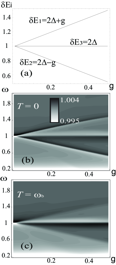
Figure 2: (a) shows the three important energy gaps, ($\delta E_{i}$, $i=1,2,3$), in the low-level energy spectrum of the Jaynes-Cummings Hamiltonian (see text). The parameter $g$ is the coupling between the electron and the resonator. (b, c) show, as contour plots, how these gaps can be observed in the current-noise frequency spectrum $S(\omega)_{e,e}/2eI_{e}$, for $\omega_{b}=1$, $\Gamma_{L}=\Gamma_{R}=0.01$, $\Delta=0.5$, $\gamma_{b}=0.05$ and $T=0,\omega_{b}$, for (b), (c), respectively. The energy gaps shown in (a) are clearly visible as three resonances in (b) and (c). The horizontal line corresponds to the physical process of an electron tunneling without exchanging quanta with the resonator. The top and bottom resonant lines are proportional to the coupling $g$, and thus represent the physical process of the electron coherently emitting a phonon into the resonator. As the temperature is increased, the visibility of the two ‘Rabi peaks’, which are signatures of coherent quantum behavior of the resonator, decreases.

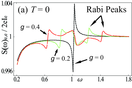
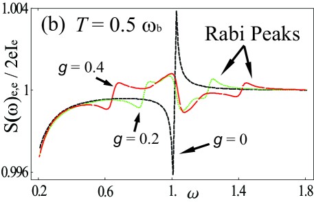
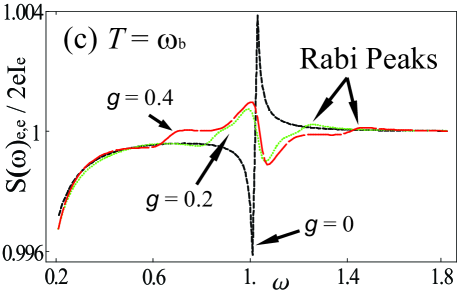
Figure 3: (color online) Normalized current-noise frequency-spectrum, $S(\omega)_{e,e}/2eI_{e}$, versus $\omega$, for $\omega_{b}=1$, $\Gamma_{L}=\Gamma_{R}=0.01$, $\Delta=0.5$, $\gamma_{b}=0.05$, and $T=0$, $0.5\omega_{b}$, $\omega_{b}$ (figures (a), (b), and (c), respectively) and a selection of electron-resonator coupling strengths $g$; black, green, red are $g=0,0.2,0.4,$ respectively. The resonances are marked by arrows. As the temperature is increased, the system enters the classical regime and the two Rabi peaks decrease and become hard to distinguish.

IV.1 First regime: effective Jaynes-Cummings Hamiltonian

An effective Jaynes-Cummings Hamiltonian can be realized if we set $\epsilon=0$ and $2\Delta=\omega_{b}$. Then,

$$H=\Delta\sigma_{x}+g\sigma_{z}(a+a^{\dagger})+\omega_{b}a^{\dagger}a.$$ (13)

Large $\Delta$ implies Brandes (2005) that there is a strong overlap between the particle wave functions in the two states, which may introduce extra coupling terms with the resonator. However, for simplicity, we assume they are negligible.

First, we write the diagonal energy term for the qubit ($\sigma_{z}$) in the off-diagonal basis ($\sigma_{x}$) by substituting raising and lowering operators in that basis

$$\sigma_{x}^{+}=\frac{1}{2}(\sigma_{z}-i\sigma_{y}),\quad\sigma_{x}^{-}=\frac{1}{2}(\sigma_{z}+i\sigma_{y}).$$ (14)

Then performing the rotating-wave approximation in this basis, by dropping counter-rotating terms, we obtain

$$H_{JC} \approx g(\sigma_{x}^{+}a+\sigma_{x}^{-}a^{\dagger})+\omega_{b}a^{\dagger}a+\Delta\sigma_{x}$$

$$= g\left[\frac{1}{2}(\sigma_{z}-i\sigma_{y})a+\frac{1}{2}(\sigma_{z}+i\sigma_{y})a^{\dagger}\right]+\omega_{b}a^{\dagger}a+\Delta\sigma_{x}.$$

This has the spectrum of an infinite number of non-interacting multiplets with eigenstates,

$$|\pm\rangle_{n}=\frac{1}{\sqrt{2}}(|n,1_{x}\rangle\pm|n+1,0_{x}\rangle,$$ (16)

where $|n\rangle$ is the number state of the mechanical resonator, and $|0\rangle_{x}$ and $|1\rangle_{x}$ are the eigenstates of $\sigma_{x}$ (i.e., the bonding and anti-bonding states within the double quantum dot).

If we consider the zero-temperature limit and a strong damping of the bath, then only the lowest number states of the mode $n=0,1$ strongly contribute to the transport processes (this case is well into the quantum regime, and the ideal situation). This regime is feasible if the effective temperature of the resonator is below $\hbar\omega_{b}$. In this case, if $\Gamma_{L}\approx\gamma_{b}$ then the initial state of each ‘round’ of transport would be

$$|\psi(t=0)\rangle=|0,L\rangle=\frac{1}{\sqrt{2}}(|0,0_{x}\rangle+|0,1_{x}\rangle.$$ (17)

The second component, $|0,1_{x}\rangle$ couples to the $n=0$ and $n=1$ states of the mechanical resonator via the $|\pm\rangle_{n=0}$ eigenstates of $H_{JC}$. The first component, $|0,0_{x}\rangle$, acts as an ‘interaction free’ transport route because it is the ground state of $H_{JC}$. The component $|0,0_{x}\rangle$ has a unique ‘ground state energy’ $E_{0}=-\Delta$, while the two $|\pm\rangle_{n=0}$ eigenstates of $H_{JC}$ have energies

$$E_{\pm}=\omega_{b}/2\pm\sqrt{\Omega^{2}+4g^{2}}/2,$$ (18)

where

$$\Omega=\omega_{b}-2\Delta.$$ (19)

Our numerical simulations in Fig. 2 and Fig. 3 show clearly how the energy level splittings $\delta E_{i}$, $(i=1,2,3)$ form resonances in the noise frequency spectrum. In particular, because $\Omega=0$ here,

$$\delta E_{1/2}=E_{\pm}-E_{0}=2\Delta\pm g$$ (20)

are the upper and lower resonance ‘branches’ in Figs. 2 and 3, caused by the coherent coupling between the double quantum dot and the mechanical resonator, and $\delta E_{3}=2\Delta$ is the central resonance because of coherent internal oscillations within the dot alone. This occurs because of the $|0,0_{x}\rangle$ ground state of $H_{JC}$, described above, which only evolves in time with a phase factor $E_{0}=-\Delta$.

As we increase the temperature of the mechanical resonator thermal bath, the upper and lower resonance branches gradually disappear, and the central resonance, determined by $\omega=2\Delta$, dominates. Increasing the temperature of the ‘bath’ means that the mechanical resonator would be in a thermal mixture of number states; thus for the electron, more transport channels become available. This is more clearly apparent in the magnitude of the noise shown in Fig. 3, illustrating that by monitoring the peaks in the current-noise transport $S_{e,e}(\omega)$ one can, in principle, distinguish classical and quantum behavior. However, the observation of near zero-temperature oscillations is not always proof of quantum behaviour Hofheinz et al. (2008); Fink et al. (2008); Schuster et al. (2008); Omelyanchouk et al. (2008); Shevchenko et al. (2008); Wei et al. (2006) as they can also be described by a classical model of coupled linear oscillators. For example, in our current-noise formulation “false signatures” from interactions of the qubit with nearby classical oscillators may appear in the spectrum and be mistaken for quantum Rabi behavior. We discuss this further in the next section.

One can understand the transition to the high-temperature case by assuming the initial state to be

$$|\psi(t=0)\rangle=\left(\sum_{n}C_{n}|n\rangle\right)\otimes\frac{1}{\sqrt{2}}\left(|0_{x}\rangle+|1_{x}\rangle\right)$$ (21)

which connects each multiplet in the spectrum of the Jaynes-Cummings Hamiltonian with its two nearest energy levels. The subspace of the Hamiltonian connecting $|n-1,1_{x}\rangle$,$|n,0_{x}\rangle$ $|n,1_{x}\rangle$ and $|n+1,0_{x}\rangle$ is (where the basis here is for $\sigma_{x}$ diagonal),

$$H_{n-1,n,n+1}=\left(\begin{array}[]{cccc}(n-1)\omega_{b}+\Delta&g\sqrt{n}&0&0\\ g\sqrt{n}&n\omega_{b}-\Delta&0&0\\ 0&0&n\omega_{b}+\Delta&g\sqrt{n+1}\\ 0&0&g\sqrt{n+1}&(n+1)\omega-\Delta\\ \end{array}\right)$$ (26)

Then, we easily see that the probability that the left dot is occupied (corresponding to the probability of the superposition of bonding and antibonding states $\frac{1}{\sqrt{2}}(|0_{x}\rangle+|1_{x}\rangle)$), is given by,

$$P_{L}(t)=\sum_{n=0}^{\infty}\left\{C_{n}\cos\left[\frac{-g(\sqrt{n+1}-\sqrt{n})t-2t\Delta}{2}\right]\right\}^{2}$$ (27)

Considering both an equal superposition, $C_{n}=1/\sqrt{N}$ (but with cut-off of the sum in $P_{L}(t)$ at a given $N$), and a coherent state distribution, $C_{n}(z)=z^{n}e^{-z}/n!$, we observe that the oscillations in the the probability $P_{L}(t)$ collapse over time, until only small oscillations with period $\Delta$ around $P_{L}=0.5$ remain. This is because the non-commensurate Rabi frequencies in Eq. [27] interfere destructively. For a small number of number states $N$, or a small coherent state distribution $z$, there is some revival in $P_{L}(t)$, but as $N$ increases the number of revivals fall. This is also true if the initial state is a separable density matrix with the resonator state in a thermal Boltzman distribution, as is the case for high-temperatures.

IV.2 Second Regime: Off-resonant interaction

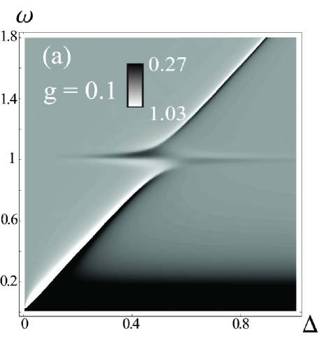
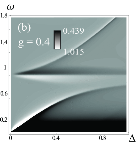
Figure 4: Current-noise frequency-spectrum, $S(\omega)_{e,e}/2eI_{e}$, versus both the tunneling rate $\Delta$ and frequency $\omega$, for (a) $g=0.1$ and (b) $g=0.4$. In both cases $\omega_{b}=1$, $\Gamma_{L}=\Gamma_{R}=0.01$, $\gamma_{b}=0.05$, $\epsilon=0$, and $T=0$. This was obtained numerically by solving the master equation in Eq. (3). As $\Delta$ approaches $\omega_{b}/2=0.5$ we see the three resonance points previously shown in Fig. 3. Increasing $g$ increases the gap between the resonant peaks. The hyperbolic behavior comes from the well know Jaynes-Cummings eigenvalue spectrum, as recently observed experimentally in a similar system (e.g., Refs [Deppe et al., 2008; Hofheinz et al., 2008; Fink et al., 2008]).

In the previous section we showed that on-resonance, $2\Delta=\omega_{b}$, the lowest part of the energy spectrum of the coupled system was visible in the current-noise. We can now verify that these resonances really stem from the low-energy spectrum of the Jaynes-Cummings Hamiltonian, and indicate coherent quantum dynamics, by inspecting the off-resonant regime, $2\Delta\neq\omega_{b}$, where the energy levels have a hyperbolic behavior. In terms of the double-dot realization, we point out that assuming a small $\Delta$ implies a tight confinement of the electron within each dot.

Observing Fig. 4(a), we can see upper and lower resonance branches, but in this case ($2\Delta\neq\omega_{b}$) they have the typical hyperbolic tails of an avoided level crossing. In addition, Fig. 4(b) shows that, as the coupling to the mechanical resonator $g$ is increased, the gap in the level crossing increases. Once more we are successfully observing the low-energy spectrum of the Hamiltonian in the power spectrum of the current-noise. For example, the upper and lower branches are simply given by the lowest eigenvalues of the Jaynes-Cummings Hamiltonian,

$$\delta E_{1,2} = |\omega_{b}/2\pm\sqrt{\Omega^{2}+4g^{2}}/2+\Delta|.$$

Furthermore, we note that there is an energy gap which halts the electron current in the limit when $\epsilon=0$ and when the coherent tunneling within the dots is small relative to the coupling to the mode, $\Delta\ll g$. This occurs because the tunneling of an electron requires an energy loss proportional to the displacement of the mode, and because the rotating wave approximation is no longer valid. For transport to occur, the electron must tunnel from the left to the right state, which is now shifted in (relative) energy by $2g(a+a^{\dagger})$. This becomes more and more difficult as the coupling $g$ is increased, resulting in a “current blockade” effect.

Finally, as discussed in the previous section, we point out that oscillations alone may not provide sufficient proof of quantum behavior. Recent circuit-QED experimentsFink et al. (2008); Hofheinz et al. (2008) have focused on the idea of observing the square-root dependence of the energy of the Jaynes-Cummings system on the photon occupation number $n$, which is sufficiently distinct from the behavior seen in classical models. However, the preparation of arbitrary Fock states in a nano-mechanical resonator is not readily realizable at this point in time.

IV.3 Zero frequency noise: comparing the single and many-mode cases

In the previous sections we showed how the low-energy levels of a Jaynes-Cummings Hamiltonian can be seen in the full-frequency current-noise spectrum. However, most recent experiments have focused on the zero-frequency noise. For example, Kießlich et al Kieszlich et al. (2007) showed, by comparing experiment and theory, that coherent oscillations in a double quantum dot produced super-Poissonian $[S(0)_{e,e}/2eI_{e}>1]$ signatures in the zero-frequency noise, while incoherent transitions (sequential tunneling induced by increasing the temperature of the phonon bath) produce sub-Poissonian noise, $[S(0)_{e,e}/2eI_{e}<1]$.

Mimicking their parameter regime, i.e. considering their device as coupled to a resonator (or phonon cavity), now we also look at the zero-frequency noise (as a function of double quantum dot level detuning $\epsilon$). We observe similar signatures to theirs in the noise spectrum, but with a more complicated structure. We also observe, in Fig.5(a), that increasing the temperature of the single mode resonator decreases the zero frequency current-noise, eventually resulting in sub-Poissonian behavior.

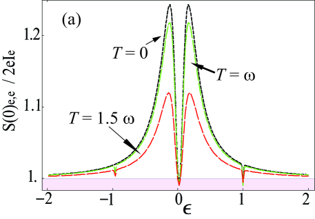
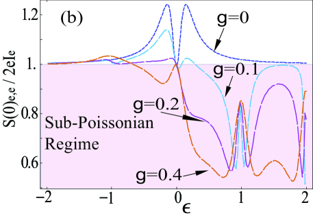
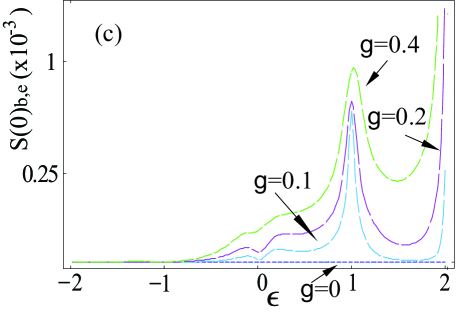
Figure 5: (Color Online) (a) Current-noise frequency-spectrum $S(0)_{e,e}/2eI_{e}$ versus $\epsilon$, for $\omega=1$, $\Gamma_{L}=0.1$, $\Gamma_{R}=0.001$, $\Delta=0.1$, $\gamma_{b}=0.01$, $g=0.0008$, increasing $T$ from $0$ to $2$ in steps of $0.5$. Increasing the temperature reduces the super-Poissonian character of the current-noise. (b) $S(0)_{e,e}/2eI_{e}$ for $\omega=1$, $\Gamma_{L}=0.1$, $\Gamma_{R}=0.001$, $\Delta=0.1$, $\gamma_{b}=0.01$, $T=0$, for $g$ from $0$ to $0.4$ in steps of $0.1$ (besides $g=0.3$, which has been omitted for figure clarity). For strong coupling we see that the current-noise becomes almost entirely sub-Poissonian (as indicated by the shaded pink region). (c) The cross-correlation $S(0)_{e,b}$ against $\epsilon$ for the same parameters as (b). Recall that $S(0)_{e,b}$ is defined as the correlation between the electron and phonon currents. For $g=0$ and for negative $\epsilon$ there is zero correlation between phonon and electron tunneling, as expected.

Similarly, increasing the bare coupling strength $g$ to the single mode resonator has a drastic effect. As Fig. 5(b) shows, the noise profile quickly becomes sub-Poissonian, developing a new peak structure around $\epsilon=1$. Interestingly, the $\epsilon=0$ point, where we earlier probed for coherent signatures, remains around $S(0)_{e,e}/2eI_{e}=1$, indicating that coherent transport is still occurring.

Figure 5(c) illustrates the (non-normalized) cross-correlated noise, i.e. the correlation between electron tunneling events and phonons leaving the mechanical resonator into a heat bath (with rate $\gamma$). As expected, there is no correlation between tunneling events when the systems are uncoupled. Furthermore, the correlated noise is large when $\epsilon=k\omega_{b}$, where $k$ is an integer. While the correlated noise grows for larger ‘$k$’, the current itself becomes smaller Brandes and Lambert (2003). This is simply because as $\epsilon$ increases, the current can only flow through phonon assisted tunneling, which happens at integer numbers of the phonon frequency.

V Squeezing the quantum state of the resonator

We have shown that the electron current-noise, $S_{e,e}(\omega)$, serves as a detector of coherent interactions between the double quantum dot and the single mode of the mechanical resonator. Already this is a significant step, as $S_{e,e}(\omega)$, serves as a tool for experimental observation. However, we can proceed a step further, and briefly consider the statistics of the phonons in the mechanical resonator. In such a mechanical system, these quantities are difficult, if not impossible, to access. However, it is informative to understand how the phonon statistics of the resonator change as we increase the temperature, and leave the quantum regime.

V.1 Squeezing signatures

In the proposal by Rodrigues et al Rodrigues et al. (2007) they show that the resonator can exhibit properties akin to a micromaser, due to the nonlinear coupling to an SSET. In their case, the qubit is represented by a superposition of island charge states $\sigma_{z}=|2\rangle\langle 2|-|0\rangle\langle 0|$. However, they focused on the regime where $\omega_{b}/\Gamma=1$, observing that this is where the interaction between the resonator and SSET is maximized. In the results we have shown in the previous sections, we assume that the quantum dots and leads are weakly coupled, $\omega_{b}/\Gamma\gg 1$. Furthermore, we assume that the resonator is strongly damped (e.g., via cooling by another SSET, or by the double quantum dot itself Grajcar et al. (2008); Ouyang et al. (2008)), so that only the few lowest bosonic levels are excited.

However, even for our ‘slow’ regime, we see sub-Poissonian signatures in the boson emission noise spectrum emitted into its nearby heat bath $S_{b,b}(0)/2I_{b}$, as well as in the Fano factor $F_{Q}$ of the number state occupation $n$ of the resonatorHu and Nori (1996a, b, 1997, 1999)

$$F_{Q}=\frac{\langle n^{2}\rangle-\langle n\rangle^{2}}{\langle n\rangle},$$ (28)

as shown in Fig. 6(a) and (b). Both ‘measures’ identify similar regions of squeezing, though there is a conceptual difference between the squeezing of the phonons emitted (dynamically) into the heat bath, and a direct measurement of the static steady-state phonon occupation number. Furthermore, we see that as the temperature is increased, both quantities increase non-linearly in magnitude.

In addition, we consider the correlated electron-phonon noise. We naively expect that stronger correlations will occur in the quantum regime. Figure 6(c) verifies this, and shows that a maximum in the correlated noise occurs around $g=0.1$, and an increase in temperature reduces the overall magnitude. This is an indication, continuing from previous suggestive results Lambert et al. (2007), that the quantum noise correlation between two open systems could serve as a measure of entanglement, though a direct correspondence has yet to be identified.

V.2 Quadrature versus number-state squeezing

The squeezing in Fig. 6 is number state squeezing, and a sub-Poissonian variance in $n$ ($F_{Q}$) implies anti-bunching of the phonon statisticsTeich and Saleh (1988). This is only one of several types of squeezing. For example, in quantum optics, generalized quadrature squeezing is often investigated. Typically the axis of squeezing might not been known, so a homodyne measurement of the occupation statistics must be performed. A homodyne measurement Mandel and Wolf (1995), using a local oscillator to introduce a relative phase, reveals the variance of any desired quadrature. Thus, in principle, it is possible to measure the normal ordered squeezing via

$$\langle:(\Delta Q)^{2}:\rangle=\langle:Q^{2}:\rangle-\langle Q\rangle^{2},$$ (29)

where $Q$ is the quadrature defined by a desired angle $\phi$, so that

$$Q=ae^{-i\phi}+a^{\dagger}e^{i\phi}.$$ (30)

Squeezing of the quadrature is implied when

$$\langle:(\Delta Q)^{2}:\rangle<0$$ (31)

for some given $\phi$, because of the normal ordering. Again, in a nanomechanical system such a measurement is not feasible, but has been proposed in transmission line resonatorsCastellanos-Beltran et al. (2008). Is is trivial to see

$$\langle:(\Delta Q)^{2}:\rangle = \langle a^{\dagger^{2}}\rangle e^{2i\phi}+\langle a^{2}\rangle e^{-2i\phi}+2\langle a^{\dagger}a\rangle$$ (32)

$$- \langle a^{\dagger}\rangle^{2}e^{2i\phi}+\langle a\rangle^{2}e^{-2i\phi}+2\langle a\rangle\langle a^{\dagger}\rangle.$$

However, for our model and parameter space, we were not able to observe any instance of quadrature squeezing. In the previous sections we discussed how strong contributions to the steady-state solution of the master equation arise from the low-level Jaynes-Cummings eigenstates. Our results illustrate that, in our system, these states only produce number state squeezing in the resonator mode, but not quadrature squeezingTeich and Saleh (1988).

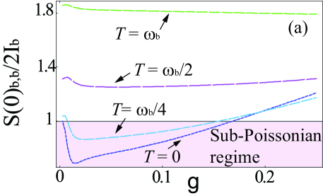
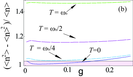
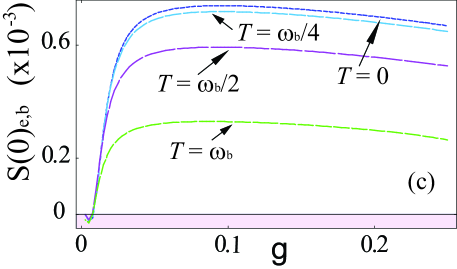
Figure 6: (Color online) (a) Bosonic current-noise frequency-spectrum, $S_{b,b}(\omega)/2I_{b}$, versus $g$, for $\omega_{b}=1$, $\Gamma_{L}=\Gamma_{R}=0.01$, $\Delta=0.5$, $\gamma_{b}=0.05$, $\epsilon=0.0$, and a range of temperatures. The pink regions [also denoted by ”Sub-Poissonian regime” in (a)] indicate the regimes where quantum state squeezing occurs, for low temperature and intermediate couplings. (b) shows the number-state Fano factor $(\langle n^{2}\rangle-\langle n\rangle^{2})/\langle n\rangle$ of the bosonic system. The zero-temperature case closely corresponds to the ‘phonon current-noise’ in (a). (c) shows the electron-phonon correlated noise $S_{e,b}(0)$ versus $g$. Interestingly, increasing the temperature decreases the correlated noise. Moreover, and as expected, the zero coupling point ($g=0$) remains around $S(0)_{e,b}=0$ for all values of temperature. Also, in a very small regime of weak coupling $(g\rightarrow 0$), $S(0)_{e,b}$ can be negative.

VI Realizations

As mentioned before, our model can correspond to charge states in a double quantum dot in a capacitively-coupled or suspended geometry. For the suspended geometryBrandes and Lambert (2003); Weig et al. (2004), it has been shown that there is a direct coupling between the electron wave function and a single phonon mode because of van-Hove singularities in the density of states. However such experiments have not yet been performed in the energy regime of the fundamental vibrational mode of a mechanical resonator. Also, our model is related to that of a superconducting single electron transistor (SSET) capacitively coupled to the resonator Naik et al. (2006); Rodrigues et al. (2007); Aguado and Brandes (2004). Typically there are some differences in the transport properties as an SSET is a three-terminal device, and the SSET drives the resonator into complex types of limit-cycle behavior Rodrigues et al. (2007); Harvey et al. (2008).

VI.1 Energy scales

To check the feasibility of our results we need to verify the appropriate energy scales in real systems. We assume that our state-of-the-art resonator has a fundamental frequency of $\omega_{b}=1$ GHz. The corresponding ‘resonant’ bias, $\epsilon=\hbar\omega$, is approximately $4$ $\mu$eV. We assume we are near the quantum limit, i.e., $kT\approx\hbar\omega_{b}$, $T\approx 50$ mK. Normal capacitive coupling strengths for an SSET are $100$ MHz, corresponding to $g=\omega/10$. In Figure 2 we saw signatures of quantum coherent oscillations for this range of coupling strengths. The same range ($g\sim\omega/10$) is feasible for the coupling between a double quantum dot and the resonator (with capacitive coupling Ouyang et al. (2008)). The achievable coupling strengths for suspended geometries are not precisely known now, but because of van-Hove singularities in the density of states one can expect large effective coupling strengths Brandes and Lambert (2003); Weig et al. (2004). Finally, the inter-state tunneling, denoted by $\Delta$ in our discussion, is typically tunable for double quantum dots. Thus a range of $\Delta\sim(1$–$10)$ $\mu$eV is feasible.

VI.2 Magnetized resonator interacting with electron spins

A recent proposal Lambert et al. (2008) focused on a magnetized resonator which interacts with one of two electron spins in a spin-blockaded double quantum dot system. In this case, the current is used to measure the spin state because, if the two spins are parallel, current cannot flow. An oscillating magnetic field, from the magnetized resonator, couples to one of the spin states, and thus this spin plays the role of a ‘transport qubit’ in our earlier language. The question of cooling such a magnetized resonator and then coupling it to a nearby electron spin via its quantized motion, and henceforth the quantized magnetic field motion, has not been addressed. In that case, the Hamiltonian of the spin and the resonator is,

$$H_{Q}=-\,\frac{\Sigma\sigma_{z}}{2}+\hbar\omega_{b}\,a^{\dagger}a+C\sqrt{\frac{\hbar}{2m_{\mathrm{eff}}\omega_{b}}}(a+a^{\dagger})\sigma_{x}$$ (33)

where $C=0.16$ mT/nm. This (Eq. 33) differs from the Hamiltonians in Eqs. 13 and IV.1 in that Eq. 33 is diagonal in the qubit energy basis. The ground state motion of a $1$ GHz resonator is $2\times 10^{-14}$ m, which, using the parameters from Ref. Lambert et al., 2008, would generate a field of just $3.2\times 10^{-6}$ mT, a Rabi frequency of about $100$ Hz, which is negligible in comparison to nuclear hyperfine and spin-orbit effects. Optimizing device design can increase this Rabi frequency considerably. For example, a larger magnetization could be achieved by using a Dysprosium (Dy) micromagnet instead of Cobalt (Co) (giving a factor of about two). Similarly, a larger micromagnet thickness could also contribute a factor of about two to the field felt by the electron spin. Decreasing the distance between the dot and resonator could contribute up to a factor of ten, and using a slower frequency resonator, for a larger ground state displacement, could add a factor of about five. Taking these factors into consideration gives a Rabi frequency in the range $10$–$100$ kHz. This Rabi frequency is still, in comparison to the charge-based quantum dot and SSET systems, a weak coupling, and is vulnerable to dephasing from nuclear hyperfine fields. However, the future evolution of this technology may make such an approach feasible and desirable, especially considering the possible benefits of combining spintronics and nanomechanics.

VII Conclusions

We have illustrated how quantum coherent behavior and the energy spectrum of a nanomechanical resonator can be identified using full-frequency current-noise measurements through a nearby transport qubit. In the zero-frequency limit, we showed that a single-mode ‘environment’, as represented by a nanomechanical resonator, produces unique signatures that differ from those observed in multi-mode environments. Furthermore, we identified regimes where phonon squeezing and cross-correlated noise, indications of complex quantum phenomena, could occur. All of these features could be realized with a double quantum dot or superconducting single-electron transistor operating as the transport qubit. In a broader context, we expect that noise measurements could also be useful in two-resonator circuit QED systemsMariantoni et al. (2005); Sun et al. (2006); Regal et al. (2008), which may offer an interesting area for future investigation.

Appendix A Noise Formalism

To calculate the quantum noise Blanter and Buttiker (2000) of a system with Hamiltonian $H$, and corresponding transport environment described by a Liouvillian $L$, we employ a generating function approach. The Master equation for the matrix elements of the generating function ${\bf g}$ is

$$\frac{\partial}{\partial t}{\bf g}(s_{1},...,s_{m},t)=M(s_{1},...,s_{m})\,{\bf g}(s_{1},...,s_{m},t),$$ (34)

which can be formally solved by diagonalizing

$$M(s_{1},...,s_{m}) =$$ (35)

$$V(s_{1},...,s_{m})D(s_{1},...,s_{m})V^{-1}(s_{1},...,s_{m}).$$

Here $M$ is the Liouvillian $L$ recast as a function of the counting variables $(s_{1},...,s_{m})$. Each $s_{i}$ is a continous variable which tracks the passage of the current through system $i$. This gives a general formalism for calculating the generating function of $m$ coherent and interacting transport systems, each with a single ‘one-way’ current flow.

The next step is to use the MacDonald formula MacDonald (1962) for the symmetrized noise power correlator between systems $i$ and $j$

$$S(\omega)_{i,j} \equiv \int_{-\infty}^{\infty}d\tau e^{i\omega\tau}\left[\langle\delta{I_{i}(t+\tau)},\delta{I_{j}(t)}\rangle\right]_{t\rightarrow\infty}$$ (36)

$$\frac{S(\omega)_{i,j}}{2e^{2}\omega} = \int_{0}^{\infty}\sin(\omega\tau)\partial_{\tau}\left(\langle n_{i}(\tau)n_{j}(\tau)\rangle-\frac{\tau^{2}\langle I_{i}\rangle\langle I_{j}\rangle}{e^{2}}\right),$$

which can be written as ($s=\{s_{1},s_{2},...,s_{m}\}$)

$$\frac{S(\omega)_{i,j}}{2e^{2}\omega} = \left(\partial_{s_{i},s_{j}}+\delta_{i,j}\partial_{s_{i}}\right)\int_{0}^{\infty}d\tau\sin(\omega\tau)$$

$$\times \frac{\partial}{\partial\tau}{\rm Tr}\hat{G}(s\tau)|_{s=1},$$

where an omitted term $2\tau\langle I\rangle^{2}$ in the integral does not contribute in the final result obtained upon performing the Laplace transformation. Noting that $\hat{G}(s,\tau=0)=\rho(0)$, where the initial condition $\rho(0)$ is the steady state density matrix and using

$$\frac{\partial}{\partial\tau}\hat{G}(s,\tau)=M(s)\hat{G}(s,\tau)=M(s)e^{\tau M(s)}\hat{G}(s,\tau=0),$$

and the spectral decomposition of $M(s)$, one obtains

$$S(\omega)_{i,j} = 2e^{2}\left(\partial_{s_{i},s_{j}}+\delta_{i,j}\partial_{s_{i}}\right)$$ (38)

$$\times \left\|V(s)\frac{\omega^{2}D(s)}{\omega^{2}+D(s)^{2}}V^{-1}(s){\bf g}(s,0)\right\|_{s=1},$$

where the notation $\left\|(x_{i_{1},j_{1}},x_{i_{2},j_{2}},...,)\right\|\equiv\sum_{i=0}x_{ii}$ takes into account the trace in  Eq. (A). Note that the first derivative in the single system correlator $\partial_{s}$ yields $2e\langle I\rangle$, and therefore $\partial_{s}^{2}$ provides the deviation from the shot noise. Using the Ramo-Shockley theorem Blanter and Buttiker (2000), the displacement current contribution can either be omitted (by assuming that the capacitances of the devices are extremely asymmetric, so that $c_{L}c_{R}\ll 1$), or calculated using a multi-variable approach, because the total current fluctuations can be written as

$$\delta I(t+\tau)\delta I(t) = \alpha^{2}\delta I_{L}(t+\tau)\delta I_{L}(t+\tau)$$ (39)

$$+ \beta^{2}\delta I_{R}(t+\tau)\delta I_{R}(t)$$

$$+ \alpha\beta(\delta I_{L}(t+\tau)\delta I_{R}(t)$$

$$+ \delta I_{R}(t+\tau)\delta I_{L}(t)).$$

The left and right correlations are trivially calculated using separate counting variables for each lead.

Equation  (38) allows one to calculate the noise spectrum for transport through an arbitrarily complex quantum system. This can be evaluated either using finite difference derivatives around $s=1$, or following the methods employed by Flindt et al. Flindt et al. (2004, 2005). In the latter case we can use their approach to show that, in general, the cross-correlator can be written as

$$\partial_{t}\langle n_{i}(t)n_{j}(t)\rangle = \text{Tr}[L_{i}\sum_{n_{1},n_{2},...}n_{j}\,\rho^{(n_{1}),(n_{2}),...}]$$ (40)

$$+ \text{Tr}[L_{j}\sum_{n_{1},n_{2},...}n_{i}\,\rho^{(n_{1}),(n_{2}),...}].$$

Furthermore the terms

$$\sum_{n_{1},n_{2},...}n_{j}\rho^{(n_{1}),(n_{2}),...}=\partial_{s_{j}}\hat{G}(s,\tau)|_{s=1}$$ (41)

can be evaluated by Laplace transforming the equation of motion

$$\partial_{\tau}\hat{G}(s,t)=(L_{0}+\sum_{i}s_{i}L_{i})\hat{G}(s,t)$$ (42)

and taking derivatives in the counting variables $s_{i}$, giving

$$\partial_{s_{i}}\tilde{G}(s,-i\omega)|_{s=1}=F(-i\omega)L_{i}F(-i\omega)\rho(0)$$ (43)

where

$$F(-i\omega)=(-i\omega-L)^{-1}$$ (44)

and $\rho(0)$ is the steady-state initial condition. As shown by Flindt et al Flindt et al. (2004) one can evaluate this inverse by writing

$$F(-i\omega) = -P/i\omega-R(\omega),$$ (45)

$$R(\omega) = Q(i\omega+L)^{-1}Q,$$ (46)

where

$$P=\rho(0)\otimes 1,\quad Q=1-P.$$ (47)

Inserting all these expressions into the cross-correlator, and using $P\rho(0)=\rho(0)$ and $Q\rho(0)=0$, gives the noise power as the trace of an inverse,

$$\frac{S(\omega)_{i,j}}{2e^{2}} = \text{Re}\left\{-\text{Tr}[L_{i}R(\omega)L_{j}\rho(0)]-\text{Tr}[L_{j}R(\omega)L_{i}\rho(0)]\right\}$$ (48)

$$+ \delta_{i,j}\text{Tr}[L_{i}\rho(0)].$$

All of the above allows us to calculate the full frequency spectrum for an arbitrary number of coupled systems. In addition, it allows us to calculate phonon current and statistics. We choose as the phonon current operator the operator which absorbs a phonon number state from the mode and puts it in the background bath.

References

- Craighead (2000) H. G. Craighead, Science 290, 1532 (2000).
- Cho (2003) A. Cho, Science 299, 36 (2003).
- Roukes and Schwab (2005) M. Roukes and K. Schwab, Physics Today 58, 7, 36 (2005).
- Treutlein et al. (2007) P. Treutlein, D. Hunger, S. Camerer, T. W. Hansch, and J. Reichel, Phys. Rev. Lett. 99, 140403 (2007).
- Wei et al. (2006) L. F. Wei, Y. X. Liu, C. P. Sun, and F. Nori, Phys. Rev. Lett. 97, 237201 (2006).
- Blencowe (2005) M. Blencowe, Contemporary Phys. 46, 249 (2005).
- Lambert et al. (2008) N. Lambert, I. Mahboob, M. Pioro-Ladriere, Y. Tokura, S. Tarucha, and H. Yamaguchi, Phys. Rev. Lett. 100, 136802 (2008).
- Rodrigues et al. (2007) D. A. Rodrigues, J. Imbers, and A. D. Armour, Phys. Rev. Lett. 98, 067204 (2007).
- Naik et al. (2006) A. Naik, O. Buu, M. D. LaHaye, A. D. Armour, A. A. Clerk, M. P. Blencowe, and K. C. Schwab, Nature 443, 193 (2006).
- Ouyang et al. (2008) S.-H. Ouyang, J. Q. You, and F. Nori, arXiv:0807.4833v1 (2008).
- Weig et al. (2004) E. M. Weig, R. H. Blick, T. Brandes, J. Kirschbaum, W. Wegscheider, M. Bichler, and J. P. Kotthaus, Phys. Rev. Lett. 92, 046804 (2004).
- Kieszlich et al. (2007) G. Kieszlich, E. Schöll, T. Brandes, F. Hohls, and R. J. Haug, Phys. Rev. Lett. 99, 206602 (2007).
- Lambert et al. (2007) N. Lambert, R. Aguado, and T. Brandes, Phys. Rev. B 75, 045340 (2007).
- Beenakker et al. (2003) C. W. J. Beenakker, C. Emary, M. Kindermann, and J. L. van Velsen, Phys. Rev. Lett. 91, 147901 (2003).
- Deppe et al. (2008) F. Deppe, M. Mariantoni, E. P. Menzel, A. Marx, S. Saito, K. Kakuyanagi, H. Tanaka, T. Meno, K. Semba, H. Takayanagi, E. Solano, R. Gross, Nature Physics 4, 686 (2008).
- Brandes and Lambert (2003) T. Brandes and N. Lambert, Phys. Rev. B 67, 125323 (2003).
- Bennett and Clerk (2006) S. D. Bennett and A. A. Clerk, Phys. Rev. B 74, 201301(R) (2006).
- Xue et al. (2007) F. Xue, Y. X. Liu, C. P. Sun, and F. Nori, Phys. Rev. B 76, 064305 (2007).
- Brandes (2005) T. Brandes, Physics Reports 408, 315 (2005).
- Aguado and Brandes (2004) R. Aguado and T. Brandes, Phys. Rev. Lett. 92, 206601 (2004).
- Blanter and Buttiker (2000) Y. M. Blanter and M. Buttiker, Physics Reports 336, 1 (2000).
- You and Nori (2005) J. Q. You and F. Nori, Physics Today 52, 11, 42 (2005).
- You and Nori (2003a) J. Q. You and F. Nori, Physica E 18, 33 (2003a).
- You and Nori (2003b) J. Q. You and F. Nori, Phys. Rev. B 68, 064509 (2003b).
- Mariantoni et al. (2005) M. Mariantoni, M. J. Storcz, F. K. Wilhelm, W. D. Oliver, A. Emmert, A. Marx, R. Gross, H. Christ, and E. Solano, arXiv:cond-mat/0509737 (2005).
- Emary et al. (2007) C. Emary, D. Marcos, R. Aguado, and T. Brandes, Phys. Rev. B 76, 161404(R) (2007).
- Flindt et al. (2008) C. Flindt, T. Novotny, A. Braggio, M. Sassetti, and A.-P. Jauho, Phys. Rev. Lett. 100, 150601 (2008).
- Hofheinz et al. (2008) M. Hofheinz, E. M. Weig, M. Ansmann, R. C. Bialczak, E. Lucero, M. Neeley, A. D. O’Connell, H. Wang, J. M. Martinis, and A. N. Cleland, Nature 454, 310 (2008).
- Fink et al. (2008) J. M. Fink, M. Göppl, M. Baur, R. Bianchetti, P. J. Leek, A. Blais, and A. Wallraff, Nature 454, 315 (2008).
- Schuster et al. (2008) I. Schuster, A. Kubanek, A. Fuhrmanek, T. Puppe, P. W. H. Pinkse, K. Murr, and G. Rempe, Nature Physics 4, 382 (2008).
- Omelyanchouk et al. (2008) A. N. Omelyanchouk, S. N. Shevchenko, A. M. Zagoskin, E. Il’ichev, and F. Nori, Phys. Rev. B 78, 054512 (2008).
- Shevchenko et al. (2008) S. Shevchenko, A. Omelyanchouk, A. Zagoskin, S. Savel’ev, and F. Nori, New J. Phys. 10, 073026 (2008).
- Grajcar et al. (2008) M. Grajcar, S. Ashhab, J. R. Johansson, and F. Nori, Phys. Rev. B 78, 035406 (2008).
- Hu and Nori (1996a) X. Hu and F. Nori, Phys. Rev. B 53, 2419 (1996a).
- Hu and Nori (1996b) X. Hu and F. Nori, Phys. Rev. Lett. 76, 2294 (1996b).
- Hu and Nori (1997) X. Hu and F. Nori, Phys. Rev. Lett. 79, 4605 (1997).
- Hu and Nori (1999) X. Hu and F. Nori, Physica B 263, 16 (1999).
- Teich and Saleh (1988) M. C. Teich and B. E. A. Saleh, Prog. In Optics XXVI 73, 022318 (1988).
- Mandel and Wolf (1995) L. Mandel and E. Wolf, Optical Coherence and Quantum Optics (Cambridge University Press, 1995).
- Castellanos-Beltran et al. (2008) M. A. Castellanos-Beltran, K. D. Irwin, G. C. Hilton, L. R. Vale, and K. W. Lehnert, Nature Physics (published online 10.1038/nphys1090) (2008).
- Harvey et al. (2008) T. J. Harvey, D. A. Rodrigues, and A. D. Armour, Phys. Rev. B. 78, 024513 (2008).
- Sun et al. (2006) C. P. Sun, L. F. Wei, Y. X. Liu, and F. Nori, Phys. Rev. A 73, 022318 (2006).
- Regal et al. (2008) C. A. Regal, J. D. Teufel, and K. W. Lehnert, Nature Physics 4, 555 (2008).
- MacDonald (1962) D. K. C. MacDonald, Noise and Fluctuations (Wiley, New York, 1962).
- Flindt et al. (2004) C. Flindt, T. Novotny, and A.-P. Jauho, Phys. Rev. B 70, 205334 (2004).
- Flindt et al. (2005) C. Flindt, T. Novotny, and A.-P. Jauho, Europhys. Lett. 69, 475 (2005).