Optimal Prediction in Molecular Dynamics

Abstract

Optimal prediction approximates the average solution of a large system of ordinary differential equations by a smaller system. We present how optimal prediction can be applied to a typical problem in the field of molecular dynamics, in order to reduce the number of particles to be tracked in the computations. We consider a model problem, which describes a surface coating process, and show how asymptotic methods can be employed to approximate the high dimensional conditional expectations, which arise in optimal prediction. The thus derived smaller system is compared to the original system in terms of statistical quantities, such as diffusion constants. The comparison is carried out by Monte-Carlo simulations, and it is shown under which conditions optimal prediction yields a valid approximation to the original system.

Keywords: Optimal prediction, molecular dynamics, surface coating, hopping, Laplace’s method, low temperature asymptotics, Monte-Carlo

1 Introduction

Computations in the field of molecular dynamics typically require a large computational effort due to two factors:

1. Small time steps are required to resolve the fast atomic oscillations.

2. Large systems are obtained due to the large amount of atoms which have to be computed.

A wide variety of methods has been developed to remedy these problems. Larger time steps are admitted e.g. by smoothing algorithms, which average in time over the fast oscillations. Various other methods reduce the degrees of freedom, e.g. multipole methods [14] in the context of long range particle interactions. In this paper we investigate whether the method of optimal prediction, as presented and analyzed in [1, 4, 5, 6, 7, 8, 9, 10, 11, 15, 19], can in principle be applied to problems in molecular dynamics in order to reduce the number of atoms to be computed. As a first step in this investigation we confine to a one dimensional model problem which inherits particular properties from a real molecular dynamics problem. In Section 2 we present the real problem as it arises in applications, and derive the simplified model problem. The considered problem is Hamiltonian, hence in Section 3 we present the method of optimal prediction in the special case of Hamiltonian systems. In Section 4 we apply the method of optimal prediction to the model problem. This yields expressions involving high dimensional integrals. We evaluate these integrals by asymptotic methods, employing the fact that the process is running at a low temperature, which yields a new and smaller system. Section 5 deals with the numerical speed-up. In Section 6 we define criteria, how to investigate whether the new system is a valid approximation to the original system. We show how important statistical quantities, such as diffusion constants and energy fluctuations, can be obtained by numerical experiments. These are presented in Section 7, and we investigate under which conditions optimal prediction preserves the relevant statistical quantities.

2 Problem Description

2.1 The Physical Problem

In the production of semiconductors a thin layer (a few atomic monolayers) of copper has to be coated (sputtered) onto a silicon crystal. A technical description of the process can be found in [18]. Important for the quality of the product is that copper atoms must not penetrate too deeply into the silicon crystal. The copper atoms penetrate firstly by their kinetic energy when hitting the crystal surface, secondly by the process of atomic hopping, which will be described in the following. In order to obtain specific knowledge about these processes, molecular dynamics simulations have to be carried out, as described in [13].

One important aspect of the coating process is that the system is out of its thermodynamical equilibrium only for very short times, namely for about $10^{-11}$ seconds after one copper atom has hit the surface of the silicon crystal. During this time the copper atom penetrates into the crystal and sonic waves transport the impact energy away to the bottom of the crystal, which is constantly being cooled. Hence, after $10^{-11}$ seconds the whole crystal is in equilibrium again. On the other hand, the time between two copper atoms hitting the crystal surface is on a time scale of $10^{-4}$ seconds, i.e. the system is in equilibrium nearly all the time, in particular the temperature is constant with respect to space and time.

However, even in the state of thermodynamical equilibrium single copper atoms can change their position in the silicon crystal by hopping events, i.e. a copper atom gains by accident enough energy to overcome the potential barrier between two layers in the silicon crystal and thus hops to a neighboring cell. By atomic hopping copper atoms can penetrate much deeper into the silicon crystal as their impact energy would allow, hence the process in equilibrium cannot be omitted from the computation. The average time between two hopping events is on a time scale of $10^{-10}$ seconds, while the fast atomic oscillations happen on a time scale of $10^{-14}$ seconds.

In this paper we show how the method of optimal prediction can be applied to the system in equilibrium. Only the atoms at the top layers of the crystal, where copper atoms can be found, are computed exactly, while the silicon atoms in the lower layers are kept track of only in an average sense. In order to keep the technical difficulties at a minimum, we set up a one dimensional model problem which simulates atomic hopping.

2.2 The Model Problem

In the model problem, we assume two major simplifications:

• Focus on a one dimensional problem, i.e. we consider $n$ atoms lined up like beads on a cord. A single copper atom is inserted into a line of $n-1$ silicon atoms.

• The potential $V(q)$ depends only on the pairwise distances of the atoms, i.e.

  $$V(q_{1},\dots,q_{n})=\sum_{\scriptstyle{i,j=1}\atop\scriptstyle{i<j}}^{n}f_{\alpha}(q_{i}-q_{j}).$$ (2.1)

  Here $\alpha\in\{1,2\}$, where $f_{1}$ is the potential between two silicon atoms and $f_{2}$ is the potential between the copper atom and a silicon atom.

Figure 1: Potential $f_{1}$ between two silicon atoms

Figure 2: Potential $f_{2}$ between copper and silicon

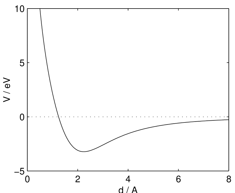
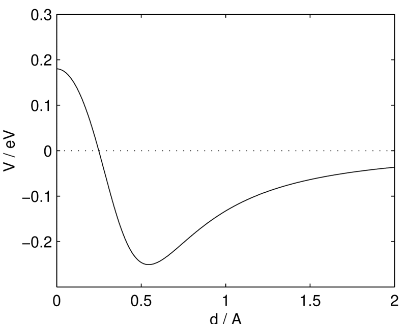
Figures 2 and 2 show the pair potentials $f_{1}$ and $f_{2}$. The distance is given in Å ($1\textrm{\AA}=10^{-10}$m) and the energy in eV ($1\textrm{eV}=1.6\cdot 10^{-19}$J). The potentials are chosen to be close to the corresponding Lennard-Jones potentials [17] in three space dimensions, in particular for $f_{1}$ the position of the minimum ($r_{e}=2.24\textrm{\AA}$) and the energy at the minimum ($E=-D$, where $D=3.24\textrm{eV}$) are chosen to fit the correct values given in [27]. In reality, hopping between two silicon atoms happens many times less likely than a copper hopping event. Hence, we neglect silicon hopping in the model problem and choose $f_{1}$ to be infinite at the origin.

On the other hand, the pair potential $f_{2}$ between copper and silicon is set to be finite at distance $0$, in order to allow copper hopping. While in a three dimensional crystal a copper atom hops through one face of a crystal cell, in one space dimension the copper atom can only hop directly over a silicon atom in order to change its position in the crystal. Additionally, the value at distance $0$ is significantly lowered compared to the potential barrier set up by a face of a three dimensional silicon crystal. This makes hopping events much more frequent and thus reduces the simulation time required for observing hopping events.

In order to further increase the hopping rate, we increase the temperature significantly. The real process is taking place at temperatures around $500\textrm{K}$. We run the simulations at a temperature of $7000\textrm{K}$, which is the maximum temperature that we can still call “low”. In this context a temperature being “low” means that the the dimensionless quantity $\varepsilon=\frac{k_{B}T}{D}$ is a small number. For real temperatures one obtains $\varepsilon\approx 0.01$, for the increased temperature $\varepsilon=0.13$. Consequently, any result obtained for increased temperatures can be expected to work even better at real temperatures.

In the following, we will always assume our system to behave as an ergodic system. In particular this means that we assume space averages over a number of atoms to be equal to time averages over a given time span.

3 Optimal Prediction for Hamiltonian Systems

Optimal prediction was introduced by Chorin, Kast and Kupferman [7] as a method to apply to underresolved computation, i.e. to problems which are computationally too expensive or where not enough data is at hand, but prior statistical information is available. Sought is the mean solution of a system, where only part of the initial data is known, and the rest is sampled from an underlying measure. While the method is in principle not restricted to a particular measure, in equilibrium statistical mechanics one typically chooses the grand canonical distribution. Optimal prediction approximates the mean solution by a new system which is smaller, and thus cheaper to compute, than the original system. In this paper we will use a simple optimal prediction system to consider only a smaller number of atoms and “averaging” the other ones away. Note that optimal prediction is by no means restricted to Hamiltonian systems, but for such systems it has some particularly nice properties.

Consider a $2n$-dimensional Hamiltonian system of ordinary differential equations

$$\dot{q}=\frac{\partial H}{\partial p},\quad\dot{p}=-\frac{\partial H}{\partial q}$$ (3.1)

with the Hamiltonian function

$$H(q,p)=\frac{1}{2}p^{2}+V(q),$$ (3.2)

representing an $n$-particle system in one space dimension. In the following, we will consider the model problem in equilibrium, hence we assume the position in state space to be distributed according to the grand canonical distribution

$$f(q,p)=Z^{-1}e^{-\beta H(q,p)}.$$ (3.3)

Here $\beta=\frac{1}{k_{B}T}$ is a constant with $k_{B}$ being the Boltzmann constant, $T$ the (constant) temperature of the process, and $Z=\int e^{-\beta H(p,q)}\,\mathrm{d}q\,\mathrm{d}p$ is a normalization constant.

We write the solution of (3.1) as a phase flow, where $\varphi(x,t)=\left(q_{1}(t),p_{1}(t),\dots,q_{n}(t),p_{n}(t)\right)$ denotes the solution to the initial condition $x=\left(\mbox{\r{q}}_{1},\mbox{\r{p}}_{1},\dots,\mbox{\r{q}}_{n},\mbox{\r{p}}_{n}\right)$. Consequently, system (3.1) can be rewritten as

$$\frac{d}{dt}\varphi(x,t) = R(\varphi(x,t)),$$ (3.4)

$$\varphi(x,0) = x.$$

Assume that only $m$ of the $n$ atoms are of interest, which yields a separation of the degrees of freedom into two groups $\varphi=(\hat{\varphi},\tilde{\varphi})$, where $\hat{\varphi}=(\varphi_{1},\dots,\varphi_{2m})$ represents the atoms of interest, and $\tilde{\varphi}=(\varphi_{2m+1},\dots,\varphi_{2n})$ corresponds to the $n-m$ atoms which should be considered only in an averaged sense. Let in the following $l=n-m$ denote the number of averaged atoms. Typically, $m$ is significantly smaller than $n$. Note that in our model problem silicon atoms cannot hop, hence this separation stays valid over time, given the copper atom stays among the silicon atoms of interest.

Now only part of the initial conditions $\hat{x}=(x_{1},\dots,x_{2m})$, namely the ones corresponding to the variables which are of interest $\hat{\varphi}$, are known, while the other components $\tilde{x}=(x_{2m+1},\dots,x_{2n})$ are not known exactly. Instead, for each choice of $\hat{x}$ they are sampled from the conditioned measure

$$f_{\hat{x}}(\tilde{x})=Z_{\hat{x}}^{-1}e^{-\beta H(\hat{x},\tilde{x})},$$ (3.5)

where $Z_{\hat{x}}=\int e^{-\beta H(\hat{x},\tilde{x})}\,\mathrm{d}\tilde{x}$ is the appropriate normalization constant. As in [5] we use the conditional expectation projection of a function $u(\hat{x},\tilde{x})$

$$Pu=\mathbb{E}[u|\hat{x}]=\frac{\int u(\hat{x},\tilde{x})e^{-\beta H(\hat{x},\tilde{x})}d\tilde{x}}{\int e^{-\beta H(\hat{x},\tilde{x})}d\tilde{x}}.$$ (3.6)

Optimal prediction as presented in [1, 4, 5, 6, 7, 8, 9, 11] is interested in the first $2m$ components of the mean solution of (3.4), where the initial conditions $\hat{x}$ are fixed and $\tilde{x}$ are sampled from (3.5)

$$P\varphi(x,t)=\mathbb{E}[\varphi(x,t)|\hat{x}]=\frac{\int\varphi((\hat{x},\tilde{x}),t)e^{-\beta H(\hat{x},\tilde{x})}d\tilde{x}}{\int e^{-\beta H(\hat{x},\tilde{x})}d\tilde{x}}.$$ (3.7)

For linear systems, expression (3.7) can be computed exactly, and it does not decay. In molecular dynamics, however, the Hamiltonian system is in general nonlinear. As observed in [1, 4], for nonlinear systems, the mean solution decays, which is interpreted as a loss of information as the first $2m$ variables tend to the thermodynamical equilibrium. In [1] the authors give a deeper physical reasoning for the decay. An application of the Mori-Zwanzig formalism as in [4, 5, 6] yields the formal explanation.

For each choice of $\hat{x}$ the mean solution (3.7) can be approximated by Monte-Carlo sampling, i.e. sampling $N$ times $\tilde{x}$ from the conditioned measure (3.5), solving $N$ times the system (3.4) with initial values $(\hat{x},\tilde{x})$, and averaging over all solutions. Obviously, this is more expensive than solving the original system itself.

In [4] the term first order optimal prediction has been assigned to idea of applying the conditional expectation projection $P$ to the right hand side $R$

$$\mathfrak{R}=PR=\mathbb{E}[R|\hat{x}],$$ (3.8)

which yields a function of just $2m$ variables. Hence, $\hat{\mathfrak{R}}=(\mathfrak{R}_{1},\dots,\mathfrak{R}_{2m})$ is a function from $\mathbb{R}^{2m}$ to $\mathbb{R}^{2m}$. The first order optimal prediction system is defined as

$$\dot{y}(t)=\hat{\mathfrak{R}}(y(t)),\quad y(0)=\hat{x}.$$ (3.9)

An important result, which allows to restrict to considering the Hamiltonian function only, is the following

Theorem 3.1 (O. Hald [10])

If a system is Hamiltonian, then its optimal prediction system is also Hamiltonian with the Hamiltonian function

$$\mathfrak{H}(\hat{q},\hat{p})=-\frac{1}{\beta}\log\left(\frac{1}{c}\int\int e^{-\beta H(\hat{q},\hat{p},\tilde{q},\tilde{p})}\,\mathrm{d}\tilde{q}\,\mathrm{d}\tilde{p}\right).$$ (3.10)

Here $c$ is a constant with unit $[c]=[\tilde{q}]\cdot[\tilde{p}]=\left(kg\frac{m^{2}}{s}\right)^{l}$. The exact value of $c$ is of no importance for the dynamics.

This theorem implies that for nonlinear problems first order optimal prediction is never a good approximation for long times, since the mean solution decays, i.e. loses energy, while the first order optimal prediction system is Hamiltonian, and thus energy preserving. In [4, 5, 6, 10] higher order optimal prediction methods have been derived, which reproduce the desired decay of the mean solution.

However, in our case, we are not interested in the mean solution, but in a $2m$-dimensional system, which yields the same behavior of the first $m$ atoms as the full $2n$-dimensional system would have yielded. This does not necessarily require a good approximation in the sense of trajectories (which the mean solution focuses on), but the relevant statistical quantities should be the recovered. In particular, the $2m$-dimensional system should be Hamiltonian again. Hence, we choose the first order optimal prediction system as the sought $2m$-dimensional system. Of course this choice can only be reasoned, if it turns out that the relevant statistical quantities are indeed preserved. We will focus on this question in Sections 6 and 7.

4 Optimal Prediction Applied to the Model Problem

4.1 Appropriate Domains of Integration

As the pair potentials $f_{1}$, $f_{2}$ vanish at infinity, the expression

$$\int_{\mathbb{R}^{n}}e^{-\beta H(x)}\,\mathrm{d}x$$ (4.1)

is not finite. Hence, the canonical measure $f(q,p)=Z^{-1}e^{-\beta H(q,p)}$ does not make sense as a probability distribution if the particle positions are not restricted in some way. In many text books on statistical mechanics the whole system is put into a box of finite volume, i.e. $\left(q_{1},\dots,q_{n}\right)\in[-L,L]^{n}$, where $L$ is suitably large. This essentially means that all atoms are trapped, but no ordering is specified. In our model problem, however, the silicon atoms are ordered, and since silicon atoms cannot hop over each other, this order stays valid over time. This is an information which we do not wish to average out. Hence, we restrict the position vector $\left(q_{1},\dots,q_{n}\right)$ to the domain

$$M^{L}=\{(q_{1},\dots,q_{n})\in[-L,L]^{n}|q_{2}<\dots<q_{n}\}.$$ (4.2)

Here $q_{1}$ is the position of the copper atom, which can be anywhere in $[-L,L]$, as it can hop freely. The positions of the silicon atoms $q_{2},\dots,q_{n}$, however, are restricted to be ordered from left to right. With respect to optimal prediction, the domain

$$M^{L}_{\hat{q}}=\{(q_{m+1},\dots,q_{n})\in[-L,L]^{l}|q_{m}<q_{m+1}<\dots<q_{n}\}$$ (4.3)

has to be introduced. For each fixed position vector $\hat{q}=(q_{1},\dots,q_{m})$ the other $l$ silicon atoms $\tilde{q}$ are restricted to be positioned right of the first $m$ atoms, and ordered. This setup assumes that the copper always stays among the first $m$ atoms.

4.2 The Optimal Prediction Hamiltonian

When considering the optimal prediction Hamiltonian (3.10) as given by Theorem 3.1, one can easily check that the kinetic and potential energy separate

$$\mathfrak{H}(\hat{q},\hat{p})=\underbrace{-\frac{1}{\beta}\log\left(\frac{1}{c_{p}^{l}}\int_{\mathbb{R}^{l}}e^{-\beta T(\hat{p},\tilde{p})}\,\mathrm{d}\tilde{p}\right)}_{=\mathfrak{T}(\hat{p})}\underbrace{-\frac{1}{\beta}\log\left(\frac{1}{c_{q}^{l}}\int_{M^{L}_{\hat{q}}}e^{-\beta V(\hat{q},\tilde{q})}\,\mathrm{d}\tilde{q}\right)}_{=\mathfrak{V}(\hat{q})}.$$ (4.4)

Here $c_{p}$ and $c_{q}$ are constants with units $[c_{p}]=\textrm{kg}\frac{\textrm{m}}{\textrm{s}}$ and $[c_{q}]=\textrm{m}$. Since $T=\frac{1}{2}\sum_{i=1}^{n}\frac{p_{i}^{2}}{m_{i}}$, the first term of (4.4) can be computed directly as

$$\mathfrak{T}(\hat{p})=\frac{1}{2}\sum_{i=1}^{m}\frac{p_{i}^{2}}{m_{i}}+C,$$ (4.5)

where the constant $C=-\frac{1}{2\beta}\sum_{i=m+1}^{n}\log\left(\frac{2\pi m_{i}}{\beta c_{p}^{2}}\right)$ is of no relevance for the dynamics. Hence, with respect to the momenta applying first order optimal prediction means omitting the momenta $p_{m+1},\dots,p_{n}$. For the potential $V$, however, life is far from being as easy as for the kinetic energy $T$, as the $q$-variables do not separate and are no quadratic functions. Thus, an analytic evaluation of the first order optimal prediction potential $\mathfrak{V}(\hat{q})$ is in general impossible, or at least too complicated to be of any use. Hence, we employ an asymptotic expansion of $\mathfrak{V}(\hat{q})$.

4.3 Low Temperature Asymptotics

The dimensionless quantity $\varepsilon=\frac{1}{D\beta}=\frac{k_{B}T}{D}$ is small for low temperatures. The optimal prediction potential expressed in terms of the quantity $\varepsilon$ is

$$\mathfrak{V}(\hat{q})=-D\varepsilon\log\left(\frac{1}{c_{q}^{l}}\int_{M^{L}_{\hat{q}}}e^{-\frac{1}{\varepsilon}\tilde{V}(\hat{q},\tilde{q})}\,\mathrm{d}\tilde{q}\right),$$ (4.6)

where $\tilde{V}(\hat{q},\tilde{q})=\frac{1}{D}V(\hat{q},\tilde{q})$ is the potential normalized in such a way, that the potential of two atoms at equilibrium distance has the value -1.

Using Laplace’s method for integrals of real variables [24, 25], one can find an asymptotic approximation to (4.6) for $\varepsilon$ small. In some textbooks this method is also referred to as Watson Lemma. Assume for the moment that for a fixed choice of $\hat{q}$ the function $\tilde{V}(\hat{q},\tilde{q})$ has a unique global minimizer $r(\hat{q})\in\mathbb{R}^{l}$ with respect to $\tilde{q}$, and that the Hessian at this point $\frac{\partial^{2}\tilde{V}}{\partial\tilde{q}^{2}}(\hat{q},r(\hat{q}))$ is regular. In the following derivation we use the abbreviatory notations $r=r(\hat{q})$ and $H_{\tilde{q}}\tilde{V}=\frac{\partial^{2}\tilde{V}}{\partial\tilde{q}^{2}}(\hat{q},r(\hat{q}))$. Laplace’s method approximates $\tilde{V}(\hat{q},\tilde{q})$ by a quadratic function located at the minimum, yielding the following asymptotic approximation for $\varepsilon\to 0$

$$\int_{M^{L}_{\hat{q}}}e^{-\frac{1}{\varepsilon}\tilde{V}(\hat{q},\tilde{q})}\,\mathrm{d}\tilde{q} \!\approx \!\int_{M^{L}_{\hat{q}}}e^{-\frac{1}{\varepsilon}\left(\tilde{V}(\hat{q},r)+\frac{1}{2}(\tilde{q}-r)^{T}\cdot H_{\tilde{q}}\tilde{V}\cdot(\tilde{q}-r)\right)}\,\mathrm{d}\tilde{q}$$

$$\!\approx \!e^{-\frac{1}{\varepsilon}\tilde{V}(\hat{q},r)}\cdot\int_{\mathbb{R}^{l}}e^{-\frac{1}{2\varepsilon}\left((\tilde{q}-r)^{T}\cdot H_{\tilde{q}}\tilde{V}\cdot(\tilde{q}-r)\right)}\,\mathrm{d}\tilde{q}.$$

Extending the set of integration to the whole $\mathbb{R}^{l}$ is valid, since the minimum is always in the interior of $M^{L}_{\hat{q}}$, provided $L$ is large enough (see [25]). Since $H_{\tilde{q}}\tilde{V}$ is assumed to be regular, the transformation rule yields

$$\frac{1}{c_{q}^{l}}\int_{\mathbb{R}^{l}}e^{-\frac{1}{2\varepsilon}(\tilde{q}-r)^{T}\cdot H_{\tilde{q}}\tilde{V}\cdot(\tilde{q}-r)}\,\mathrm{d}\tilde{q}=\sqrt{\frac{(2\pi\varepsilon)^{l}}{\left|\det c_{q}^{2}H_{\tilde{q}}\tilde{V}\right|}}.$$ (4.7)

Given $\tilde{V}$ is of class $C^{2}$ (which is the case in our model problem), the complete asymptotic expansion including the error term is

$$\frac{1}{c_{q}^{l}}\int_{M^{L}_{\hat{q}}}\!\!e^{-\frac{1}{\varepsilon}\tilde{V}(\hat{q},\tilde{q})}\,\mathrm{d}\tilde{q}=\sqrt{\frac{(2\pi\varepsilon)^{l}}{\left|\det c_{q}^{2}H_{\tilde{q}}\tilde{V}\right|}}\!\cdot\!e^{-\frac{1}{\varepsilon}\tilde{V}(\hat{q},r)}+e^{-\frac{1}{\varepsilon}\tilde{V}(\hat{q},r)}\!\cdot\!O\left(\varepsilon^{\frac{l}{2}+1}\right),$$ (4.8)

which follows directly from the one dimensional case as shown in [24, pp. 33-34]. Substituting (4.8) into (4.6), and employing that $\log(1+x)\sim x$ as $x\to 0$ yields

$$\mathfrak{V}(\hat{q})=V(\hat{q},r)+C+\frac{D\varepsilon}{2}\log\left|\det c_{q}^{2}H_{\tilde{q}}\tilde{V}\right|+O\left(\varepsilon^{2}\right),$$ (4.9)

where the constant $C=-\frac{1}{2}Dl\varepsilon\log\left(2\pi\varepsilon\right)$ is of no relevance for the dynamics. Hence, we found a zeroth and a first order asymptotic expansion in $\varepsilon$ for $\mathfrak{V}$, which – returning to long notation – are

$$\mathfrak{V}_{0}(\hat{q}) = V(\hat{q},r(\hat{q})),$$ (4.10)

$$\mathfrak{V}_{1}(\hat{q}) = V(\hat{q},r(\hat{q}))+\varepsilon\cdot\frac{D}{2}\log\left|\det\frac{c_{q}^{2}}{D}\frac{\partial^{2}V}{\partial\tilde{q}^{2}}(\hat{q},r(\hat{q}))\right|.$$ (4.11)

Note that $\mathfrak{V}_{0}$ and $\mathfrak{V}_{1}$ approximate $\mathfrak{V}$ only up to constants, which are irrelevant for the acting forces. Whenever in the following we speak of $\mathfrak{V}_{i}$ approximating $\mathfrak{V}$, we always mean: “up to constants”.

The above assumptions, that $\tilde{V}(\hat{q},\tilde{q})$ has a unique global minimizer $r(\hat{q})$ with respect to $\tilde{q}$, and that the Hessian at this point $\frac{\partial^{2}\tilde{V}}{\partial\tilde{q}^{2}}(\hat{q},r(\hat{q}))$ is regular, can be observed to be guaranteed for our model problem, given one restricts to the domain $M^{L}_{\hat{q}}$. Both assumptions can be relaxed for the zeroth order expansion, i.e. also in the case of multiple minimizers or a singular Hessian the zeroth order expansion stays valid.

4.4 Zero Temperature Limit

The zeroth order approximation $\mathfrak{V}_{0}$ (4.10) is the limit of $\mathfrak{V}$ (4.6) as $\varepsilon\to 0$, i.e. $T\to 0$. Hence, we call $\mathfrak{V}_{0}$ the zero temperature limit potential. Since the dynamics takes place at low temperatures, one can expect the correct optimal prediction potential function $\mathfrak{V}$ to be close to the zero temperature limit potential $\mathfrak{V}_{0}$. Hence, we run the low temperature optimal prediction dynamics, which would be correctly described by $\mathfrak{V}$, with the zero temperature limit dynamics given by $\mathfrak{V}_{0}$. We do not consider the first order approximation (4.11) here, since the Hessian $\frac{\partial^{2}\tilde{V}}{\partial\tilde{q}^{2}}(\hat{q},r(\hat{q}))$ cannot be included in a straightforward manner into the following derivation. The results in Subsection 7.3, however, will show that further investigation on the first order expansion could be worthwhile.

By going over from $\mathfrak{V}$ to $\mathfrak{V}_{0}$ we have formally replaced an $l$-dimensional integration by an $l$-dimensional minimization problem. At first glance this is no real improvement, since high dimensional global minimization is also computationally expensive (see [20]). However, the $l$-dimensional minimization means nothing else than placing $l$ further atoms, such that the total potential energy is minimized. Since $\mathfrak{V}_{0}$ is formally $m$-dimensional, we call the $l$ new atoms virtual atoms. The restriction to the domain $M^{L}_{\hat{q}}$ in Subsection 4.1 guarantees that the $l$ virtual atoms are separated from the $m$ “real” atoms.

4.5 Equations of Motion

The zero temperature limit Hamiltonian is

$$\mathfrak{H}_{0}(\hat{q},\hat{p})=\mathfrak{T}_{0}(\hat{p})+\mathfrak{V}_{0}(\hat{q})=\frac{1}{2}\hat{p}^{T}\mathfrak{M}^{-1}\hat{p}+V(\hat{q},r(\hat{q})),$$ (4.12)

where $\mathfrak{M}$ is a diagonal matrix containing the masses $m_{i}$ of the atoms $(\mathfrak{M})_{ii}=m_{i}$. In the following we assume $V(\hat{q},r)$ and $r(\hat{q})$ to be of class $C^{1}$. This allows to compute

$$\frac{\partial\mathfrak{H}_{0}}{\partial\hat{p}}(\hat{q},\hat{p}) \!\!= \!\!\frac{\partial\mathfrak{T}_{0}}{\partial\hat{p}}(\hat{p})=\mathfrak{M}^{-1}\cdot\hat{p},$$ (4.13)

$$\frac{\partial\mathfrak{H}_{0}}{\partial\hat{q}}(\hat{q},\hat{p}) \!\!= \!\!\frac{\partial\mathfrak{V}_{0}}{\partial\hat{q}}(\hat{q})=\frac{\partial V}{\partial\hat{q}}(\hat{q},r(\hat{q}))+\underbrace{\frac{\partial V}{\partial r}(\hat{q},r(\hat{q}))}_{=0}\cdot\frac{dr}{d\hat{q}}(\hat{q})=\frac{\partial V}{\partial\hat{q}}(\hat{q},r(\hat{q})).$$ (4.14)

Note that $\frac{\partial V}{\partial r}(\hat{q},r(\hat{q}))$ is zero, since $r(\hat{q})$ is the minimizer of $V(\hat{q},r(\hat{q}))$. Still, expression (4.14) involves a minimization problem, in order to place the virtual atoms. We circumvent the minimization by deriving equations of motion for the virtual atoms, too. In order to obtain the expression $\frac{\partial r}{\partial\hat{q}}(\hat{q})$, we define

$$v(\hat{q}):=\frac{\partial V}{\partial\tilde{q}}(\hat{q},r(\hat{q})).$$ (4.15)

Since $r(\hat{q})$ is always chosen to minimize $V$, we have that $v(\hat{q})=0~{}\forall\hat{q}$. Thus

$$0=\frac{\partial v}{\partial\hat{q}}(\hat{q})=\frac{\partial^{2}V}{\partial\hat{q}\partial\tilde{q}}(\hat{q},r(\hat{q}))+\frac{\partial^{2}V}{\partial\tilde{q}^{2}}(\hat{q},r(\hat{q}))\cdot\frac{\partial r}{\partial\hat{q}}(\hat{q}).$$ (4.16)

Solving (4.16) for $\frac{\partial r}{\partial\hat{q}}(\hat{q})$ yields an expression which can be substituted into the time evolution $\frac{d}{dt}r(\hat{q})=\frac{\partial r}{\partial\hat{q}}(\hat{q})\cdot\frac{d\hat{q}}{dt}$. This yields a closed system for the zero temperature limit optimal prediction dynamics

$$\frac{d}{dt}\hat{q} = \mathfrak{M}^{-1}\cdot\hat{p}$$

$$\frac{d}{dt}\hat{p} = -\frac{\partial V}{\partial\hat{q}}(\hat{q},r(\hat{q}))$$ (4.17)

$$\frac{d}{dt}r = -\left(\frac{\partial^{2}V}{\partial\tilde{q}^{2}}(\hat{q},r(\hat{q}))\right)^{-1}\cdot\frac{\partial^{2}V}{\partial\hat{q}\partial\tilde{q}}(\hat{q},r(\hat{q}))\cdot\mathfrak{M}^{-1}\cdot\hat{p},$$

where initially $\hat{q}_{i}(0)=q_{i}(0)$ and $\hat{p}_{i}(0)=p_{i}(0)$ and $r(0)$ is chosen such that $V(\hat{q}(0),r(0))$ is minimal, which can be resolved by a few Newton steps.

Since the virtual atoms always follow the minimum of the potential energy, no momenta are required to describe their movement. Hence, system (4.17) is just $(n+m)$-dimensional, instead of $2n$-dimensional. It is a closed system of ordinary differential equations, and the right hand side requires no integration or minimization. Still, there is an $l$-dimensional linear system of equations to be solved. At this point, we can employ the special structure of the potential energy (2.1) in our problem.

Assume that the pair potentials $f_{1}$, $f_{2}$ reach over only $k$ (in our model problem $k\approx 10$) equilibrium distances $d_{0}$. In the following derivation, we assume the potentials to really vanish at greater distances. The derived results hold approximately also for potentials which are negligibly small at greater distances. Consequently, only the first $k$ virtual atoms $r_{m+1},\dots,r_{m+k}$ actually have to be computed. The others will align equidistantly right to the first $k$ ones. Since one atom has no influence on atoms more than $k$ equilibrium distances away, only $l=2k$ virtual atoms need to be considered, where the last $k$ ones are aligned equidistantly. As we are interested in the case $m\ll n$, enough virtual atoms are present, such that boundary effects can be neglected. Let the positions of the $2k$ virtual atoms be denoted by

$$r=\left(\begin{array}[]{c}r^{V}\\ r^{E}\end{array}\right),$$ (4.18)

where $r^{V}=\left(r_{m+1},\dots,r_{m+k}\right)^{T}$ and $r^{E}=r_{m+k}e+\left(d_{0},2d_{0},\dots,kd_{0}\right)^{T}$ with $e=\left(1,\dots,1\right)^{T}$. The time derivative is

$$\frac{d}{dt}r=\left(\begin{array}[]{c}\dot{r}^{V}\\ \dot{r}_{m+k}e\end{array}\right).$$ (4.19)

In this setup the matrices in (4.17) take a special structure:

• The Hessian $\frac{\partial^{2}V}{\partial\tilde{q}^{2}}(\hat{q},r(\hat{q}))$ is a diagonal band matrix with band width $k$. In block form, where each block is of size $k\times k$, it is

  $$\frac{\partial^{2}V}{\partial\tilde{q}^{2}}(\hat{q},r(\hat{q}))=\left(\begin{array}[]{cc}A_{11}&A_{12}\\ A_{21}&A_{22}\end{array}\right),$$ (4.20)

  where $A_{12}$ is lower triangular and $A_{21}$ upper triangular.

• The matrix $\frac{\partial^{2}V}{\partial\hat{q}\partial\tilde{q}}(\hat{q},r(\hat{q}))$ is upper triangular with width $k$, i.e.

  $$\frac{\partial^{2}V}{\partial q_{i}\partial q_{m+j}}(\hat{q},r)=f^{\prime\prime}(r_{j}-q_{i})\begin{cases}=0&\text{if }|m+j-i|>k\\ \neq 0&\textrm{else}\end{cases}$$ (4.21)

  In block form it can be written as

  $$\frac{\partial^{2}V}{\partial\hat{q}\partial\tilde{q}}(\hat{q},r(\hat{q}))=\left(\begin{array}[]{cc}0&B_{12}\\ 0&0\end{array}\right),$$ (4.22)

  where $B_{12}$ is an upper triangular $k\times k$ matrix.

Substituting these special vectors and matrices into the equation for the virtual atoms in (4.17) yields the following equation of motion in block form

$$\left(\begin{array}[]{cc}A_{11}&A_{12}\\ A_{21}&A_{22}\end{array}\right)\cdot\left(\begin{array}[]{c}\dot{r}^{V}\\ \dot{r}_{m+k}e\end{array}\right)=\left(\begin{array}[]{cc}0&B_{12}\\ 0&0\end{array}\right)\cdot\mathfrak{M}^{-1}\cdot\hat{p},$$ (4.23)

which implies the $k$-dimensional system for $r^{V}$

$$\bar{A}_{11}\cdot\dot{r}^{V}=B_{12}\cdot\mathfrak{M}_{l}^{-1}\cdot\hat{p}_{l}.$$ (4.24)

Here $\bar{A}_{11}=A_{11}+\left(A_{12}\cdot e\right)\cdot e_{k}^{T}$, where $e_{k}=\left(0,\dots,0,1\right)^{T}$. The momenta of the last $k$ real atoms are denoted by $\hat{p}_{l}=\left(p_{m-k+1},\dots,p_{m}\right)^{T}$, and $\mathfrak{M}_{l}$ is the diagonal matrix containing the corresponding masses. This relation can be interpreted as a boundary layer condition which acts as if the crystal of silicon atoms was continued to infinity, although it is actually cut off after the $m$-th atom.

With the above modifications the zero temperature limit optimal prediction system (4.17) becomes an explicit $(2m+k)$-dimensional system of equations. Hence, one can expect this system to yield a computational speed-up, depending on the values of $n$, $m$ and $k$. The question of speed-up will be considered in Section 5. Due to the various approximations in achieving the smaller system it is not at all clear whether the smaller system yields the same dynamics as the original system. In Section 6 we will compare the new system to the original system and investigate under which conditions the new system reflects the “correct” dynamics, and under which conditions it does not.

5 Computational Speed-Up

Besides the above physical interpretations, the actual intention was to use optimal prediction as a method to reduce the computational effort. In this section, we consider both the version with $l$ virtual atoms and the boundary layer version. We compare the CPU times for computations of the two optimal prediction systems with the CPU time for the corresponding computations of the original system. The comparison is carried out in dependence of the sizes $n$ and $m$. Since the original version of optimal prediction does only replace real atoms by virtual ones, while on the other hand the boundary layer condition version allows to really omit atoms, a significant speed-up can only be expected from the boundary layer condition version.

Figure 3: Speed-up factors depending on $n$ and $m$.

Figure 4: Speed-up factors for $n=2m$

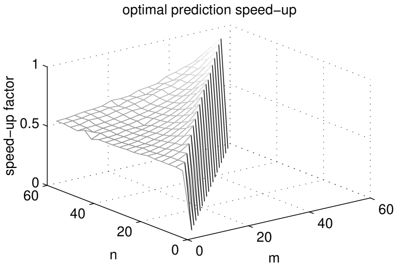
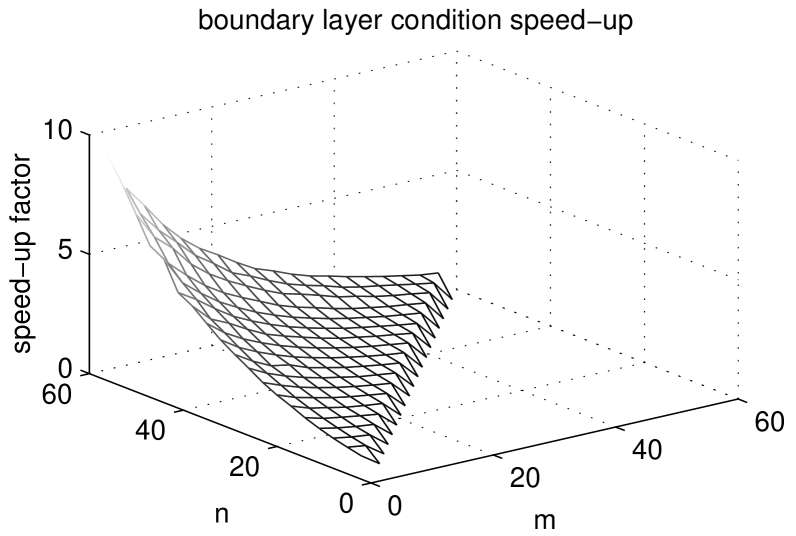
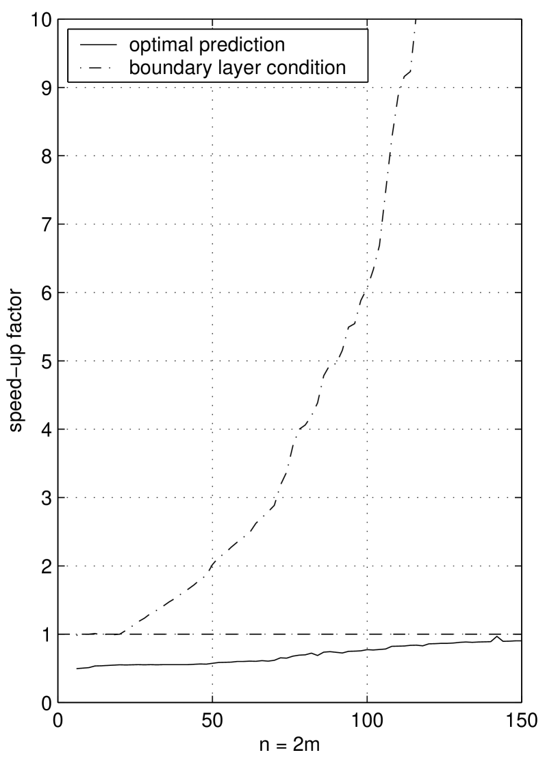
The computations were performed on a network of AMD Athlon-6 1.4 GHz computers. The boundary layer condition version was computed with $k=10$ virtual atoms. Figure 4 shows the speed-up factors with respect to the original system for the two versions of optimal prediction. The original version of optimal prediction does not yield any acceleration (the speed-up factors are less than 1). Apparently, for our model problem setting up and solving the linear system in (4.17) is more expensive than computing the full system of equations. The boundary layer condition version, on the other hand, yields significant speed-up factors for small $m$. In principle, one can achieve arbitrarily high speed-up factors by keeping $m$ and $k$ fixed and increasing $n$. In most cases, however, the original crystal size $n$ is given a priori, and suitable values for $m$ are given by the requirement that the new system must have the same dynamics as the original one, as discussed in Section 6.

A choice of $m$ which is reasonable in many cases, is cutting the whole crystal of $n$ atoms into two halves, i.e. $m=\lfloor\frac{n}{2}\rfloor$. The speed-up factors for the two optimal prediction systems are shown in Figure 4. While the original version does not reduce the computational effort, the boundary layer condition version yields a good speed-up for larger $n$.

Care should be taken when generalizing these results. In our model problem the potential functions are fairly cheap to evaluate. In more complicated systems it could very well pay off to solve the linear system in (4.17) instead, or to solve the minimization problem directly. On the other hand, the boundary layer condition version of optimal prediction could possibly fail to work in other applications, e.g. in three space dimensions. Such questions will have to be investigated when applying optimal prediction to a new problem.

6 Comparing Two Molecular Dynamics Systems

In molecular dynamics trajectories in high dimensional phase space are no appropriate means for comparing two systems, since initial positions and momenta can never be known exactly, and molecular dynamics is typically chaotic. Instead, “comparing” means to test whether both systems have similar dynamics. This is represented by statistical quantities such as time correlation functions, diffusion constants, fluctuations of energy, etc. We consider the following statistical processes in order to compare the two systems:

• The distribution of the position the copper atom. A copper atom, which is initially located always at the same position, is in the ensemble of many experiments described by a diffusion process, whose distribution can be approximated by Monte-Carlo sampling.

• The number of hopping events up to a fixed time.

• The fluctuation of energy of the first $\mathbf{m}$ atoms. The energy of the first $m$ atoms fluctuates around some fixed average. We consider the variance of the energy over a fixed time interval.

The first two quantities are related to the diffusion of a single copper atom in the silicon crystal due to hopping events. Since copper hopping has been the effect of interest in the first place, it is a natural criterion for comparison.

In molecular dynamics, statistical quantities of ergodic systems can be computed by long time averaging or Monte-Carlo sampling. “Long time averaging” means running a single computation and using limiting processes to approximate statistical quantities. Important examples, e.g. for approximating self-diffusion constants [2], are the Green-Kubo formula [17, 23] or the Einstein relation, which both approximate ensemble averages for ergodic systems by long time averaging. In our application, however, long-time computations are problematic, since firstly the copper atom may travel to the boundaries of the silicon crystal and secondly sonic waves will come in effect, as shown in Section 7. Hence, we obtain the diffusion constant by Monte-Carlo sampling instead, i.e. we solve the same system over and over again with short computation times, where the initial conditions are sampled from the canonical measure. In other words: We obtain the averaged quantities not by long-time averaging, but by averaging over many samples.

Sampling both the initial positions $q_{i}$ and momenta $p_{i}$ from the canonical measure $Z^{-1}e^{-H(q,p)}$ would require expensive methods like acceptance-rejection methods or Metropolis sampling [12, 16] due to the structure of the potential $V(q)$. We circumvent such problems by setting the initial positions $q_{i}$ into the potential minimum and sampling the initial momenta $p_{i}$ from $\tilde{Z}^{-1}e^{-T(p)}$, which is just sampling independently from Gaussian distributions. In our simulations after about $5\cdot 10^{-14}\textrm{s}$ the Hamiltonian dynamics has driven the system into equilibrium. Additionally, keeping the initial positions fixed automatically guarantees to remain in the correct domain $M^{L}$ as given by (4.2).

6.1 A Random Walk Model for the Copper Diffusion

The considered copper diffusion is due to hopping events, while displacements due to short oscillations between the same two silicon atoms are not taken into account. Hence, the corresponding diffusion process is discrete in space on the spatial grid $\{-\nu d_{0},\dots,0,\dots,\nu d_{0}\}$. Let us assume for the moment, that the diffusion process is linear and hence described by a $(2\nu+1)$-dimensional compartment model

$$\dot{u}(t)=A\cdot u(t),\quad u(0)=e_{m+1}=\left(0,\dots,0,1,0,\dots,0\right)^{T},$$ (6.1)

where $A\in\mathbb{R}^{\left(2\nu+1\right)\times\left(2\nu+1\right)}$ has column sums equal to zero to ensure mass conservation, i.e. $\frac{d}{dt}\sum_{i}u_{i}(t)=0$. The analytical solution to (6.1) is

$$u(t)=\exp(tA)\cdot e_{m+1}.$$ (6.2)

One example for such a process is given by the tridiagonal Toeplitz (up to the boundary entries) matrix with the stencil $\frac{\kappa}{d_{0}^{2}}\left(1,-2,1\right)$, which is a finite difference approximation to the heat equation. Hence, the compartment model (6.1) with this matrix converges to the heat equation as $d_{0}\to 0$. Still, there are many other matrices $A$, whose discrete diffusion processes all converge to the heat equation as $d_{0}\to 0$.

The hopping behavior of the copper atom can be modeled as a specific random walk. One important aspect of the copper hopping is that hopping events are correlated, in the sense that given the copper atom has just hopped, it is much more likely than normally that a second hopping event to the same direction follows, since the kinetic energy is not completely lost in one single jump. Hence, the copper diffusion is formally non-Markovian. Still, the hopping can be described as a Markovian random walk by assuming hopping events to be uncorrelated, but to allow the copper atom to hop over more than one silicon atom in one single hopping event.

These assumptions lead to a model which is typical in the context of stochastic processes, see [22]. Let $X_{t}$ denote the position of the copper atom at time $t$. For the $n^{\mathrm{th}}$ hopping event let $T_{n}$ be the hopping time, $\Delta T_{n}=T_{n}-T_{n-1}$ the time since the previous hopping event, and $\Delta_{n}\in\mathbb{Z}\setminus\{0\}$ the number of silicon atoms which the copper atoms hops over to the right. Here $\Delta_{n}<0$ means hopping to the left. Assume now that both the $\Delta T_{n}$ and the $\Delta_{n}$ are independent and distributed according to

$$P\left(\Delta T_{n}\in[s,s+\,\mathrm{d}s)\right)=\alpha\cdot\exp(-\alpha s)\,\mathrm{d}s,$$ (6.3)

$$P\left(\left|\Delta_{n}\right|=i\right)=p_{i}.$$ (6.4)

Here $\alpha$ is a parameter controlling the hopping rate (see [21, 22] for a derivation), and $(p_{i})_{i\in\mathbb{N}}$ is a non-negative sequence satisfying $\sum_{i\in\mathbb{N}}p_{i}=\frac{1}{2}$ and the constant $\gamma=\sum_{i=1}^{k}(d_{0}i)^{2}p_{i}$ is finite. For our model problem we simply assume $p=\left(p_{1},\dots,p_{k}\right)$. Additionally, we restrict to symmetric random walks, which is reasonable as long as the copper atom does not approach the crystal boundaries.

An analysis of the described random walk, following the analysis in [22], yields that the variance of the process at time $t$ equals $\textrm{Var}(X_{t})=2\gamma\alpha t$. A comparison with the variance given by the heat equation yields the relation

$$\kappa=\gamma\alpha,$$ (6.5)

which allows us to speak consistently of a diffusion constant $\kappa$ also for the discrete diffusion process (6.1). As derived in [22] the probability distribution of the random walk $X_{t}$ is described by (6.1), where the so called infinitesimal generator $A$ is a band matrix with the stencil $\alpha\cdot\left(p_{k},\ldots,p_{1},-1,p_{1},\ldots,p_{k}\right)$. Define $\tilde{A}$ as a corresponding band matrix with the stencil $\gamma^{-1}\cdot\left(p_{k},\ldots,p_{1},-1,p_{1},\ldots,p_{k}\right)$, hence $A=\kappa\tilde{A}$. Both matrices have to be changed in the upper and lower rows according to the appropriate boundary conditions.

Assume now, that the values $p_{1},\dots,p_{k}$ are known. Hence, the matrix $\tilde{A}$ is completely determined. Let $v(t)\in\mathbb{R}^{2\nu+1}$ denote the numerically obtained distribution vectors for the position of the copper atom for all times $t$. Initially $v(0)=e_{m+1}$, as in (6.1). Since it is unclear, whether the diffusion parameter $\kappa$ is constant in time, we let it be a time dependent parameter $\kappa(t)$, which we compute at times $t_{1},\dots,t_{\mu}$. For obtaining the value $\kappa_{j}=\kappa(t_{j})$ we consider the diffusion on the time interval $I_{j}=[\underline{t}_{j},\overline{t}_{j}]$, where $\underline{t}_{j}=t_{j}-\frac{\Delta t}{2}$ and $\overline{t}_{j}=t_{j}+\frac{\Delta t}{2}$. Given $\Delta t$ is not too large, we can approximately assume the diffusion parameter to be constant on the given interval: $\kappa(\tau)=\kappa_{j}\forall\tau\in I_{j}$. On $I_{j}$ we use the data provided by the real evolution $v(t)$ to compute an $\mathbb{L}^{2}$-fit of the diffusion parameter $\kappa_{j}$ with respect to error functional

$$F(\kappa_{j})=\int_{\underline{t}_{j}}^{\overline{t}_{j}}\|e^{(\tau-\underline{t}_{j})\kappa(t_{j})\tilde{A}}\cdot v(\underline{t}_{j})-v(\tau)\|_{2}^{2}\,\mathrm{d}\tau,$$ (6.6)

which is particularly stable with respect to errors in $v$ due to the Monte-Carlo sampling. The time $\Delta t$ must on the one hand be small enough to justify the approximation that the diffusion parameter is constant on the intervals $I_{j}$, on the other hand it must be large enough to have already some diffusion taken place. In Subsection 7.1 we compute diffusion parameters for the numerical data obtained for our model problem.

7 Numerical Experiments

We simulate a crystal of $n=70$ atoms with $69$ silicon atoms and $1$ copper atom, which starts at the $22^{\mathrm{nd}}$ position. For the optimal prediction system, we choose $m=50$. These are enough atoms such that averaged quantities make sense and one can speak of a thermodynamical equilibrium. Additionally, the crystal has a reasonable interior region which is not affected by any boundary effects. The integration is performed by the classical explicit fourth order Runge-Kutta method, which we prefer over energy preserving methods in this context, as it allows significantly larger time steps, while still resolving the hopping events accurately. The integration time step is $\Delta t=2.5\cdot 10^{-15}\textrm{s}$, and the computation time is $t^{*}=4.0\cdot 10^{-13}\textrm{s}$, which is short enough, such that the change in total energy due to the integrator is insignificant. We solve the system $N=25000$ times at a temperature $T=7000\textrm{K}$, with the initial data sampled as described in Section 6. For our experiments, Monte-Carlo estimates yield an expected error in the distribution of about $4\cdot 10^{-3}$, which is significantly smaller than the difference of any two quantities in comparison.

Note that the short computation time $t^{*}$ allows to exclude any effects caused by sonic waves traveling through the crystal. The velocity of sound can be estimated as derived in [17]: The equilibrium distance inside the silicon crystal is approximately $d_{0}=1.87\cdot 10^{-10}\textrm{m}$. Using the Young modulus $Y=d_{0}\cdot\frac{\partial^{2}H_{\textrm{loc}}}{\partial d_{0}^{2}}(d_{0})=5.05\cdot 10^{-9}\textstyle\frac{\textrm{kg}\cdot\textrm{m}}{\textrm{s}^{2}}$ we obtain a velocity of sound of $c=\sqrt{\frac{Y\cdot d_{0}}{m_{Si}}}=4.50\cdot 10^{3}\textstyle\frac{\textrm{m}}{\textrm{s}}$. The shortest distance of the copper atom to any boundary in the crystal is $s_{\textrm{left}}=q_{22}-q_{1}=2.01\cdot 10^{-9}\textrm{m}$ in the original system and $\tilde{s}_{\textrm{right}}=q_{50}-q_{22}=1.90\cdot 10^{-9}\textrm{m}$ in the optimal prediction system. Hence, the minimum time a sonic wave takes to travel from a boundary to the copper atom is approximately $t_{\textrm{min}}=\tilde{s}_{\textrm{right}}/c=4.22\cdot 10^{-13}\textrm{s}$, which is longer than the computation time $t^{*}=4.0\cdot 10^{-13}\textrm{s}$. In Subsection 7.4 we will deal with the case when sonic waves are present.

Figure 5: Distribution of the copper atom’s position

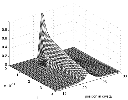
Figure 5 shows the distribution of the position of the copper atom in the silicon crystal when solving the original system. The analogous distribution for the optimal prediction system looks indistinguishably similar in this kind of plot. The process is apparently of a diffusive nature, but the diffusion parameter changes with time, as already the evolution of the maximum indicates. The following analysis will confirm this observation.

The time-dependent relative error between the distributions for the original and the optimal prediction system

$$e(t)=\frac{\max_{x}|v(x,t)-\tilde{v}(x,t)|}{\max_{x}|v(x,t)|}$$ (7.1)

is less than 3% up to the time $t=3.0\cdot 10^{-13}\textrm{s}$ and still less than 9% over the complete time interval, which is not overwhelmingly small, but does indicate definite similarities between the two distributions.

7.1 Diffusion Parameters

We compute the diffusion parameters $\kappa(t)$ for the original and the optimal prediction system, using the method described in Subsection 6.1. The parameters $(p_{1},\dots,p_{k})$ of the corresponding random walk model are obtained by Monte-Carlo sampling. We use the experiments for the original system, which already yielded the distribution shown in Figure 5. In each Monte-Carlo experiment we follow the path of the copper atom and cluster consecutive hopping events which happen in an interval of $\Delta t_{1}=6.0\cdot 10^{-14}\textrm{s}$ to a single one. Prior to this clustering, fast double hopping events into opposing directions, i.e. those happening inside of $\Delta t_{2}=2.0\cdot 10^{-14}\textrm{s}$, which are solely due to oscillations of silicon atoms, must be excluded. The times $\Delta t_{1}$ and $\Delta t_{2}$ are suitably chosen for our model problem.

The results of the above described Monte-Carlo experiments are shown in Figure 7. The hopping probabilities are given by the box histogram. Note that due to Monte-Carlo errors and boundary effects the resulting values are not exactly symmetric. Since we wish to consider a symmetric random walk, we choose as $p_{1},\dots,p_{k}$ the average values of the obtained results. Here, only $p_{1},\dots,p_{11}$ are greater than zero. Hence, we choose $k=11$ for the computation of the diffusion parameters. The curve denotes the values $i^{2}p_{i}$ (scaled to fit into the same plot), which are relevant, since the variance $\sum_{i=1}^{k}i^{2}p_{i}=\frac{\gamma}{d_{0}^{2}}$ is proportional to $\kappa$ (see relation (6.5)).

Figure 6: Probabilities of hopping over more than a single atom

Figure 7: Diffusion parameters over time

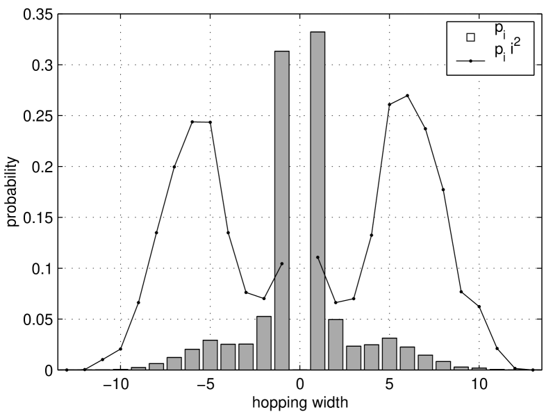
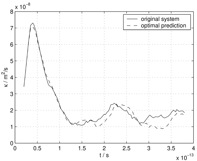
Figure 7 shows the time-dependent diffusion parameter $\kappa(t)$ for the original system and the optimal prediction approximation, computed as described in Subsection 6.1. In both cases we choose $\Delta t=2.5\cdot 10^{-14}\textrm{s}$. Important observations and estimates are:

• The diffusion parameters start with a strong peak, and after $1\cdot 10^{-13}\textrm{s}$ they fluctuate around a fixed value of $\kappa=4.4\cdot 10^{-10}\frac{m^{2}}{s}$. This behavior is too pronounced to be only due to Monte-Carlo and approximation errors. The initial behavior is most likely due to the fact that the system does not exactly start in its thermodynamical equilibrium.

• Considering that $\kappa(t)$ shows such pronounced behavior, the two functions $\kappa(t)$ for the original system, and $\tilde{\kappa}(t)$ for the optimal prediction approximation are remarkably close to each other. Up to the time $t=1.4\cdot 10^{-13}\textrm{s}$ the the distance between the two curves is quite small. After that time the curves differ more, but show the same features. After $3.0\cdot 10^{-13}\textrm{s}$ the error takes its maximum, which coincides with the errors observed in the distributions shown in Figure 5.

• In order to roughly estimate whether the obtained diffusion parameter is reasonable, we compare it with a diffusion coefficient measured in a real material. In [3] the diffusion constant of copper in a silicon crystal at a temperature of $T_{0}=1273\textrm{K}$ is given as $\kappa_{0}=4.4\cdot 10^{-10}\frac{m^{2}}{s}$. Assuming that the diffusion constant depends linearly both on temperature and the potential barrier, as e.g. with the Einstein formula [17], we obtain an estimate $\kappa\approx\kappa_{0}\cdot\frac{T}{T_{0}}\cdot\frac{\Delta E_{0}}{\Delta E}=1.7\cdot 10^{-8}\textstyle\frac{m^{2}}{s}$ for $T=7000\textrm{K}$, using the values $\Delta E_{0}=3\textrm{eV}$ and $\Delta E=0.43\textrm{eV}$. A look at Figure 7 indicates that our experimentally obtained diffusion parameters are indeed in this region.

7.2 The Number of Hopping Events

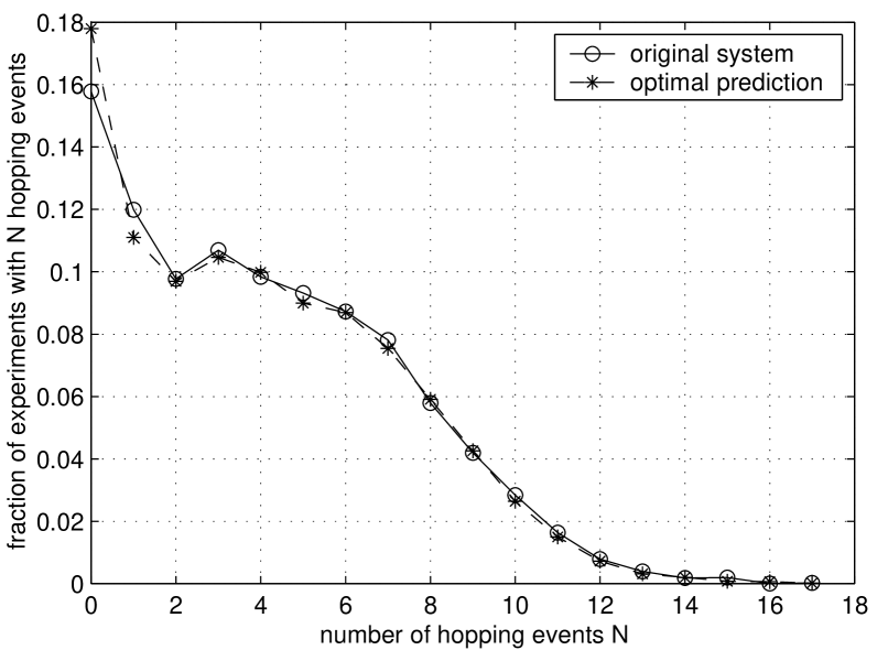
Besides diffusion parameters, also the pure number of hopping events which happen up to a given time $t^{*}$ should be preserved by optimal prediction. Figure 9 shows the number of hopping events for the above computation plotted as histograms. The solid line represents the original system, and the dashed line stands for the optimal prediction system. The two graphs differ only for the probabilities of zero and one hopping event. Apart from that, one can speak of the same hopping behavior.

Figure 8: Number of hopping events

Figure 9: Total energy fluctuation

7.3 Energy Fluctuations

While the total energy is constant for the original system as well as for the optimal prediction approximation, the energy of the first $m$ atoms

$$E_{\textrm{left}}(t)=\frac{1}{2}\sum_{i=1}^{m}\frac{p_{i}^{2}(t)}{m_{i}}+\sum_{\scriptstyle{i,j=1}\atop\scriptstyle{i<j}}^{m}f_{\alpha}(q_{i}(t)-q_{j}(t))$$ (7.2)

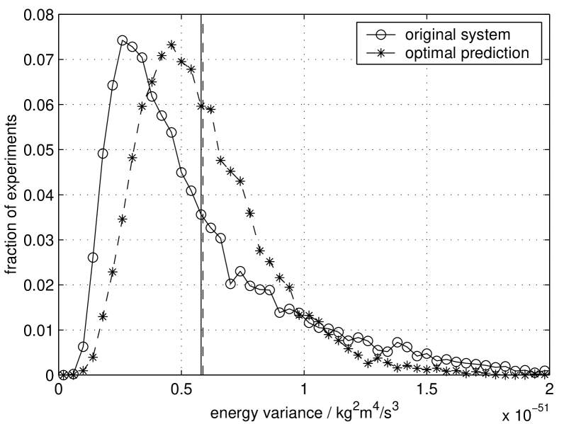
fluctuates over time. This expression fluctuates also for the optimal prediction system, since the influence of the virtual atoms is neglected in the potential energy. The fluctuations in (7.2) represent the exchange of energy between atoms, which is a quantity that should be preserved. Since for optimal prediction we consider the energy of exactly the real atoms, this test enlightens the exchange of energy between real and virtual atoms. For each Monte-Carlo experiment we consider the variance of (7.2) over time

$$V=\int_{t=0}^{t^{*}}\left(E_{\textrm{left}}(t)-E_{\textrm{left}}(0)\right)^{2}\,\mathrm{d}t,$$ (7.3)

which measures the impact of fluctuation. Hence, we obtain $N$ values $V_{1},\dots,V_{N}$ for both the original system and the optimal prediction approximation.

Figure 9 shows the histogram for the variances $V_{i}$ for the two systems. The solid line stands for the original system, and the dashed line corresponds to optimal prediction. The average energy fluctuations for both systems are denoted by the corresponding vertical lines. While the average fluctuations are very close for the two systems and the two distributions look similar in principle, they obviously do not coincide. For optimal prediction most energy fluctuations are stronger than for the original system. On the other hand, particularly high energy fluctuations happen more frequently in the original system. Possible physical reasons for this behavior could be:

• The fact, that in optimal prediction most fluctuations are stronger than in the original system might be due to the additional fluctuative Langevin terms, which appear in higher order optimal prediction [4].

• The high fluctuations in the original system can happen, since around the $m^{\mathrm{th}}$ atom energy can be exchanged freely among a whole cluster of atoms. In the zeroth order approximation to optimal prediction (4.10), on the other hand, there is no free energy exchange between the virtual atoms, since they have no momentum, but instead always follow the potential minimum. Using the first order asymptotic expansion (4.11) might remedy this problem.

Additionally, at correct temperatures ($T=500\textrm{K}$ instead of $T=7000\textrm{K}$) the energy fluctuations in optimal prediction might be much closer to the truth, even for the zeroth order approximation.

7.4 Sonic Waves

In the above experiments care was taken to exclude sonic waves, which was done by keeping the computation time shorter than a wave would take to travel through half the crystal. If the computation time is quadrupled and the diffusion distribution analogous to the one shown in Figure 5 is computed, one can indeed observe a small antidiffusive peak every $5\cdot 10^{-13}\textrm{s}$, i.e. in many experiments the copper atom is systematically pushed back to its starting position. The fact that the above time equals approximately the time a sonic waves takes for traveling from the crystal boundaries to the copper atom gives rise to the assumption that the observed behavior is indeed due to sonic waves.

The relevance of sonic waves for optimal prediction can be seen if one lets a sonic wave run into the boundary between real and virtual atoms. The wave does not penetrate into the block of virtual atoms, but is being reflected by them. Hence, optimal prediction simulates a crystal continued to infinity only as long as the system is in thermodynamical equilibrium. Non-equilibrium effects, in particular sonic waves, are not reproduced correctly by the optimal prediction system in the presented form. Indeed, in the presence of sonic waves optimal prediction yields a very different copper diffusion, unlike the experiments where sonic waves were excluded. Thus the influence of non-equilibrium effects has to be considered carefully when optimal prediction is applied to other problems.

8 Conclusions and Outlook

In this paper, we applied the method of optimal prediction to a model problem in the context of molecular dynamics, focusing on diffusion due to atomic hopping. Employing the fact that the temperature of the process is low, asymptotic methods were applied to evaluate the conditional expectations which arise in optimal prediction. The zeroth order asymptotic expansion was used to derive a new system of equations, which is formally smaller. Since in molecular dynamics potentials typically range only over short distances, the new system could be cut off after a boundary layer of virtual atoms. This boundary layer condition acts as if the crystal was continued to infinity, and yields an obvious computational speed-up for our model problem. The asymptotic method itself should apply to much more general cases than the specific model problem here.

In order to investigate whether the thus derived system preserves the statistical behavior of the original system, various criteria were introduced and checked by Monte-Carlo experiments. In particular, the diffusion of a copper atom in the crystal as well as the number of hopping events turned out to be preserved well. The exchange of energy at the boundary layer was not preserved that well, but this discrepancy could be explained. On the other hand, the new system yielded significantly worse results in the presence of non-equilibrium effects, in particular sonic waves, since optimal prediction assumes the system to be in equilibrium.

A natural next step in research on this topic would be to apply the method to a more complex problem, possibly in three space dimensions and with focus on further effects than atomic hopping. The basic ideas presented in this paper should also apply in three space dimensions, but various aspects will become more problematic. On the other hand, in three space dimensions sonic waves should dissipate faster, and the fraction of atoms which can be averaged out would be larger. Additionally, the relevant statistical quantities should be approximated much better at physically correct temperatures. An obvious step for deriving a more accurate system is to employ the first order asymptotic expansion, which was derived in Section 4. Of particular interest in this context is the question, how to generalize the method of optimal prediction to problems not in equilibrium.

We have shown that optimal prediction can in principle be applied to problems in molecular dynamics which take place at comparably low temperatures and are in equilibrium. The boundary condition version yielded an obvious speed-up. While the pure speed-up is not overwhelming by itself, the physical interpretation of the optimal prediction equations should allow to apply the method in combination with other methods. Further investigation may improve the derived results.

References

- [1] J. Bell, A.J. Chorin and W. Crutchfield, Stochastic optimal prediction with application to averaged Euler equations, Proc. 7th Nat. Conf. Comput. Fluid Mech., C.A. Lin (ed), Pingtung, Taiwan, pp. 1-13, 2000.
- [2] B.J. Berne, J.D. Gezelter, E. Rabani, Calculating the hopping rate for self-diffusion on rough potential energy surfaces: Cage correlations, J. Chem. Phys. 107, No. 17, pp. 6867-6876, 1997.
- [3] L.J. Chen, S.L. Cheng, H.H. Lin, The failure mechanisms and phase formation for Ni, Co and Cu contacts on ion implanted (001)Si under high current stress, Nucl. Instr. and Meth.in Phys. Res. B 169, pp. 161-165, 2000.
- [4] A.J. Chorin, O. Hald and R. Kupferman, Optimal prediction and the Mori-Zwanzig representation of irreversible processes, Proc. Nat. Acad. Sc. USA, 97, pp. 2968-2973, 2000.
- [5] A.J. Chorin, O. Hald and R. Kupferman, Non-markovian optimal prediction, Monte Carlo Methods and Applications, Vol. 7, No. 1-2, pp. 99-109, 2001.
- [6] A.J. Chorin, O. Hald and R. Kupferman, Optimal prediction with memory, Physica D 166, No. 3-4, pp. 239-257, 2002.
- [7] A.J. Chorin, A. Kast and R. Kupferman, Optimal prediction of underresolved dynamics, Proc. Nat. Acad. Sc. USA, 95, pp. 4094-4098, 1998.
- [8] A.J. Chorin, A. Kast and R. Kupferman, Unresolved computation and optimal prediction, Comm. Pure Appl. Math., 52, pp. 1231-1254, 1999.
- [9] A.J. Chorin, A. Kast and R. Kupferman, On the prediction of large-scale dynamics using unresolved computations, Contemp. Math., 238, pp. 53-75, 1999.
- [10] A.J. Chorin, Probability, mechanics, and irreversibility, Lecture notes, UC Berkeley Math. Dept., 2000.
- [11] A.J. Chorin, R. Kupferman and D. Levy, Optimal prediction for Hamiltonian partial differential equations, J. Comput. Phys., 162, pp. 267-297, 2000.
- [12] L. Devroye, Non-uniform random variate generation, Springer, 1986.
- [13] T. Frauenheim, H. Hensel, P. Klein, H.M. Urbassek, Comparison of classical and tight-binding molecular dynamics for silicon growth, Phys. Rev. B 53, pp. 16497-16503, 1996.
- [14] L. Greengard, V. Rokhlin, A fast algorithm for particle simulations, J. Comp. Physics, 73, pp. 325-348, 1987.
- [15] O. Hald and R. Kupferman, Convergence of optimal prediction for nonlinear Hamiltonian systems, SIAM J. Num. Anal. 39, pp. 983-1000, 2001.
- [16] J.M. Hammersley, D.C. Handscomb, Monte Carlo methods, Chapman and Hall, 1979.
- [17] J. P. Hansen, I. R. McDonald, Theory of simple liquids, Academic Press, London, 1976.
- [18] S. Hasegawa, S. Ino, Z.H. Zhang, Epitaxial growth of Cu onto Si(111) surfaces at low temperatures, Surface Science 415, pp. 363-375, 1998.
- [19] A. Kast, Optimal prediction of stiff oscillatory mechanics, Proc. Natl. Acad. Sci. USA 97, No.12, pp. 6253-6257, 2000.
- [20] S. Kirkpatrick, C.D. Gelatt Jr, M.P. Vecchi, Optimization by Simulated Annealing, Science, V. 220, No. 4598, pp. 671-680, 1983.
- [21] U. Krengel, Einführung in die Wahrscheinlichkeitstheorie und Statistik, Vieweg, 1991.
- [22] G.F. Lawler, Introduction to stochastic processes, Chapman and Hall, London, 1995.
- [23] M.H. Lee, Fick’s law, Green-Kubo formula, and Heisenberg’s equation of motion, Physical Review Letters, Col. 85, No. 12, pp. 2422-2425, 2000.
- [24] J.D. Murray, Asymptotic analysis, Springer, 1984.
- [25] F.W.J. Olver, Asymptotics and special functions, Academic Press, 1974.
- [26] B. Seibold, Optimal prediction in molecular dynamics, Diploma Thesis, University of Kaiserslautern, 2003.
- [27] B.M. Smirnov, A.S. Yatsenko, Properties of dimers, Phys. Usp. 39, No. 3, pp. 211-230, 1996.