Chaos in a one-dimensional integrable quantum system

Abstract.

We study a simple one-dimensional quantum system on a circle with $n$ scale free point interactions. The spectrum of this system is discrete and expressible as a solution of an explicit secular equation. However, its statistical properties are nontrivial. The level spacing distribution between its neighboring odd and even levels displays a surprising agreement with the prediction obtained for the Gaussian Orthogonal Ensemble of random matrices.

¹ University of Hradec Králové, Hradec Králové - Czech Republic
² Institute of Physics, Academy of Sciences of the Czech Republic,
Prague - Czech Republic
³ Doppler Institute for Mathematical Physics and Applied Mathematics,
Faculty of Nuclear Sciences and Physical Engineering, Czech Technical University, Prague - Czech Republic
⁴ Department of Physics, Faculty of Nuclear Sciences and Physical Engineering,
Czech Technical University, Prague - Czech Republic

1. Introduction

One possible approach to study the chaotic properties of bounded time-independent quantum system is based on results of the Random matrix theory (RMT). Bohigas, Giannoni and Schmit [1] conjectured that the local fluctuations of quantum energy levels of such systems display universal properties. Following this conjecture the level spacing distribution of integrable systems with more than one degree of freedom is expected to be Poissonian, while the distribution for systems that are classically chaotic is described by the random matrix theory (see [2]). (Integrability in the quantum case means that the eigenvalues and eigenvectors of the system can be evaluated by solving a simple algebraic equation.) The specific distribution depends in this case on the symmetry of the system and is described by the Gaussian orthogonal, unitary or symplectic ensemble respectively. Nowadays there is an impressive amount of evidence for the relevance of this conjecture and so for the link between the random matrix theory and the quantum behaviour of classically chaotic systems.

The assumption about the number of degrees of freedom is, however, quite important since the conjecture doesn’t hold in one dimension. All classical time independent one dimensional systems are integrable. Nevertheless there are quasi one-dimensional quantum systems (the quantum graphs) that display random matrix properties. Recent papers give a wide theoretical and experimental evidence for such behaviour in various interconnected quantum graphs [3, 4, 5, 6]. The quantum dynamic is here related to the nontrivial topological structure of the graph and the random matrix description of the spectral statistics of the quantum graph is based on this fact.

Quantum graphs are topologically nontrivial since each node is connected with at least three neighbors. This is why these systems are regarded as quasi one dimensional. In a very one dimensional system each point is topologically related only to its two neighbors: to the one on its right and to the one on its left. Our aim here is to construct a virtually one dimensional system (i.e. each node has only 2 neighbors) displaying a random matrix behavior. The work is based on the paper [11]. However there is a great difference in results. We focus on the weak coupling limit and show that in this case, the level-spacing spectral statistic display two fundamentally different types of behavior. The statistical properties of the odd level spacings are described by the random matrix theory while the even spacings do not show this behavior.

We deal with a one dimensional particle on a circle with scale free point interactions localized at the points $0<x_{1}<\ldots<x_{n}<2\pi$. The scale free point interaction ([7, 8]) localized at the origin is described by a one parameter family of boundary conditions: $\frac{1}{\alpha}f(0_{-})=f(0_{+}),\quad\alpha f^{\prime}(0_{-})=f^{\prime}(0_{+}).$ It has the amazing property that the corresponding reflection / transmission coefficients do not depend on the particle energy. The scale free point interaction is also expressible as a limit of short-range potentials, see [9, 10].

The Hamiltonian of the system is represented by the one dimensional Laplace operator

(1) $$T_{\alpha}=-\frac{d^{2}}{dx^{2}}$$

with a set of boundary conditions:

(2) $$f(2\pi_{-})=f(0_{+}), f^{\prime}(2\pi_{-})=f^{\prime}(0_{+}),\quad$$

(3) $$\frac{1}{\alpha}f(x_{k-})=f(x_{k+}), \quad\alpha f^{\prime}(x_{k-})=f^{\prime}(x_{k+}),\ k=1,\ldots,n,$$

where $\alpha\in(0,+\infty)$ is a parameter. We denote the domain of $T_{\alpha}$ as $D(T_{\alpha})$. The periodic boundary conditions (2) define a circle. The second pair (3) describes the point interactions. It can be easily shown (see the theory of self adjoint extensions e.g.[12]) that the operator $T_{\alpha}$ is self adjoint for every $\alpha$. Moreover, its spectrum is purely discrete containing eigenvalues of finite multiplicity without limit points. Note that for $\alpha=1$ the Hamiltonian describes simply a free particle on a circle. Furthermore in the limits $\alpha\rightarrow 0,\ \alpha\rightarrow+\infty$ the system decouples into $n$ independent subsystems with the Dirichlet boundary condition on one side and the Neumann condition on the other side of the subintervals $(x_{k},x_{k+1})$.

2. The spectrum

In what follows we will focus on the positive part of the spectrum denoting $x_{0}=0$ and $x_{n+1}=2\pi$. An eigenvector $\varphi_{k},k>0$ corresponding to the energy $E=k^{2}$ writes on the subinterval $(x_{j},x_{j+1}),\ j=0,\ldots,n$ as

(4) $$\varphi_{k}(x)=A_{j}(k)e^{ikx}+B_{j}(k)e^{-ikx},$$

with some coefficients $A_{j}$ and $B_{j}$. The vector $\varphi_{k}(x)$ belongs to the domain $D(T_{\alpha})$ if it satisfies the boundary conditions (2) and (3). This leads to a relation between the neighboring coefficients $A_{j-1},\ B_{j-1}$ and $A_{j},\ B_{j}$

$${A_{j}\choose B_{j}}=\boldsymbol{C}_{j}{A_{j-1}\choose B_{j-1}}.$$

for each $j=1,\ldots,n$, with $C_{j}$ being a 2x2 matrix:

(5) $$\boldsymbol{C}_{j}=\frac{1}{2}\left(\begin{array}[]{cc}\left(\frac{1}{\alpha}+\alpha\right)&\left(\frac{1}{\alpha}-\alpha\right)e^{-i2kx_{j}}\\ \left(\frac{1}{\alpha}-\alpha\right)e^{i2kx_{j}}&\left(\frac{1}{\alpha}+\alpha\right)\end{array}\right).$$

The dependence between $A_{n},\ B_{n}$ and $A_{0},\ B_{0}$ is given by the periodic boundary conditions (2) and leads to a relation

(6) $${A_{0}\choose B_{0}}=\boldsymbol{C}_{P}{A_{n}\choose B_{n}}$$

with matrix

(7) $$\boldsymbol{C}_{P}=\left(\begin{array}[]{cc}e^{i2k\pi}&0\\ 0&e^{-i2k\pi}\end{array}\right).$$

Combining all these relations together we obtain that the coefficients $A_{0},\ B_{0}$ determine an eigenvector of $T_{\alpha}$ iff

(8) $$\left(\boldsymbol{C}_{P}\boldsymbol{C}_{n}\cdots\boldsymbol{C}_{1}-\boldsymbol{I}\right){A_{0}\choose B_{0}}=0.$$

So the eigenvalues of $T_{\alpha}$ are obtained as solutions of the equation

(9) $$\zeta_{P}(k)\equiv\mathrm{det}\left(\boldsymbol{C}_{P}\boldsymbol{C}_{n}\cdots\boldsymbol{C}_{1}-\boldsymbol{I}\right)=0.$$

Since the matrices in the above determinant are of size $2\times 2$, we can easily determine the explicit form of (9) from (5) and (7) by induction. The secular equation becomes

(10) $$\zeta_{P}(k)=\cos(2k\pi)-(1-\beta^{2})^{\frac{n}{2}}+\beta^{2}\sum_{k<l}^{n}\cos(2k(x_{k}-x_{l}+\pi))+\beta^{4}\ldots=0$$

where

(11) $$\beta=\frac{1-\alpha^{2}}{1+\alpha^{2}}.$$

Note that (10) is a finite series and it ends when the number of indices in the last sum reaches the highest even number $m$ with $m<n$. So the last term is

(12) $$\beta^{m}\sum_{i_{1}<\ldots<i_{m}}^{n}\cos(2k(x_{i_{1}}-x_{i_{2}}+\ldots+x_{i_{m-1}}-x_{i_{m}}+\pi)).$$

Since the equation (10) contains only even powers of $\beta$ the positive spectrum of $T_{\alpha}$ is invariant under the replacement $\alpha\leftrightarrow 1/\alpha$ (it leads to the change $\beta\leftrightarrow-\beta$).

In the free case ($\alpha=1;\beta=0$) the equation (10) simplifies to

(13) $$\zeta_{P}(k)=\cos(2k\pi)-1=0$$

and the solutions are just

(14) $$k_{l}=l,\qquad l\in\mathbb{N},$$

with the eigenvalues being doubly degenerate (a consequence of the rotational symmetry of the system).

3. Statistical properties of the spectrum

We start with the free case omitting its non degenerate ground state. Further we suppose that all the points $0<x_{1}<\ldots<x_{n}<x_{n+1}=2\pi$ are rationally independent, i.e. we suppose that the equation

(15) $$\sum_{i=1}^{n+1}m_{i}x_{i}=0,\quad m_{i}\in\mathbb{Z}$$

has a solution only for $m_{i}=0$ for all $i$.

The states are two times degenerate. Since we want to compare the fluctuation properties of the energy levels with the random matrix theory we will not work directly with the eigenvalues $E_{l}=k_{l}^{2}$ but with the values $e_{l}=2|k_{l}|$. The point is that the values $e_{l}$ have not to be unfolded and are of density 1. From now on whenever we deal with the level spacing statistics we have the ”spectrum” $e_{l}$ in mind.

The free case is trivial: $e_{2l-1}=e_{2l}=2l,l=1,2,...$. Defining the level spacing $s_{l}=e_{l+1}-e_{l}$ we immediately see that the probability density $P(s)$ consists simply of two delta peaks $P(s)=(\delta(s)+\delta(s-2))/2$. The peak at $0$ comes from the degeneracy of the eigenvalues.

The question is what happens in the case $\alpha\neq 1$, i.e. when the point interactions are switched on. The degeneracy vanishes and the two delta peaks turn into smooth distributions.

To see what happens in that case let us assume a small change of the parameter $\alpha$ :

$$\alpha=1+\delta$$

with $\left|\delta\right|\ll 1$. The relation (11) leads to

$$\beta=\frac{1-\alpha^{2}}{1+\alpha^{2}}=(-\delta)\frac{2+\delta}{2+2\delta+\delta^{2}}\approx-\delta.$$

So the secular equation (10) can be solved perturbatively supposing the roots $k_{j}$ in the form

(16) $$k_{j}=j+\beta\lambda_{j},\ j\in\mathrm{N}\cup\{0\}$$

with $|\beta\lambda_{j}|\ll 1$. Substituting it into the equation ((10)) and using the properties of goniometric functions we get

$$1-\frac{4\pi^{2}\beta^{2}\lambda^{2}_{j}}{2}+\ldots-1+\frac{n}{2}\beta^{2}+$$

$$+\beta^{2}\sum_{k<l}^{n}\cos(2j(x_{k}-x_{l}))\left(1-\frac{4\beta^{2}\lambda^{2}_{j}(x_{k}-x_{l}+\pi)^{2}}{2}+\ldots\right)-$$

$$-\beta^{2}\sum_{k<l}^{n}\sin(2j(x_{k}-x_{l}))\left(2\beta\lambda_{j}(x_{k}-x_{l}+\pi)-\ldots\right)+\beta^{4}\ldots=0.$$

The absolute term drops out and we get (in the order of $\beta^{2}$)

$$-2\pi^{2}\lambda_{j}^{2}+\frac{n}{2}+\sum_{k<l}^{n}\cos(2j(x_{k}-x_{l}))=0.$$

The solutions $\lambda_{j}$ are given by

(17) $$\lambda^{\pm}_{j}=\pm\frac{1}{2\pi}\sqrt{\left(\sum_{k=1}^{n}\cos(2jx_{k})\right)^{2}+\left(\sum_{k=1}^{n}\sin(2jx_{k})\right)^{2}}.$$

The degenerate eigenvalues split and become

(18) $$k_{2j-1}=j+\left|\beta\right|\lambda^{-}_{j},\quad\quad k_{2j}=j+\left|\beta\right|\lambda^{+}_{j}\quad\quad j=1,2,...$$

So the unfolded level spacings are

(19) $$s_{2j-1}=4\left|\beta\right|\lambda^{+}_{j},\quad s_{2j}=2-2\left|\beta\right|(\lambda^{+}_{j+1}+\lambda^{+}_{j}).$$

The odd spacings $s_{2j-1}$ contribute to the widening of the $\delta-$ peak localized at $0$ while the even spacings $s_{2j}$ broaden the $\delta$ peak localized at 2. We will now show that the peak at 0 is not only broaden but it acquires a shape prescribed by the random matrix theory.

The positions $x_{i}$ and $\pi$ are altogether rationally independent. Hence $x_{i}/\pi$ are also rationally independent irrational numbers. The periodicity of cosine leads to the relation

$$\cos(2jx_{i})=\cos(2jx_{i}\ \mathrm{mod}\ 2\pi)=\cos(2\pi((jx_{i}/\pi)\ \mathrm{mod}\ 1)),$$

where mod means the remainder after integer division. From the theory of distribution of sequences modulo one (see [13]) we know that when $j$ changes the arguments of cosines and sines in (17) behave like independent random variables uniformly distributed in $[0,2\pi)$. From this fact follows that the distribution of the sequence $\{\cos(2jx_{i})\}_{j=1}^{+\infty}$ has a probability density function

(20) $$f(x)=\left\{\begin{array}[]{lc}\frac{1}{\pi\sqrt{1-x^{2}}},&x\in(-1,1),\\ 0,&x\in\mathbb{R}\setminus(-1,1).\end{array}\right.$$

Moreover for different positions $x_{i}$, $i=1,\ldots,n$ these sequences behave like independent random variables. The same holds for $\{\sin(2jx_{k})\}_{j}$. So the sums $\{\sum_{k=1}^{n}\cos(2jx_{k})\}_{j}$, $\{\sum_{k=1}^{n}\sin(2jx_{k})\}_{j}$ normalized by the factor $\sqrt{2}/\sqrt{n}$ converge with increasing $n$ to two normally distributed random variables.

In fact there two variables are statistically independent. To see this we sketch the proof of this fact. It is based on the observation that the pair $\left(\cos(X),\sin(X)\right)$, with $X$ being uniformly distributed along $(0,2\pi)$, can be equivalently represented in the form

$$\left(\mathrm{sgn}(\cos X)|\cos X|,\mathrm{sgn}(\sin X)\sqrt{1-|\cos X|^{2}}\right).$$

As one can easily prove, random variables $\mathrm{sgn}(\cos X),\mathrm{sgn}(\sin X)$ and $|\cos X|$ are stochastically independent. So the statistical dependence of the cosine and sine is fully contained in their absolute values, while their signs are statistically independent. This observation together with the characteristic function technique used in the standard proof of the Central limit theorem shows finally the statistical independence of the above sums.

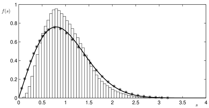
Summarizing we see that in the weak perturbation limit the distribution of the odd spacings $s_{2j-1}$ is given by a square root of a sum of squares of two independent and normally distributed random variables. Properly normalized it is nothing but the Wigner distribution $P_{W}$ approximating the spacing distribution $P_{GOE}$ of the Gaussian orthogonal ensemble of random matrices (GOE):

(21) $$P_{W}(s)=\frac{\pi}{2}se^{-\pi s^{2}/4}.$$

Remember that during the limiting procedure the perturbation condition $|\beta\lambda_{j}|\ll 1$ has to be fulfilled for every $n$. Together with the structure of the formula (17) it leads to a condition $|\beta|\ll 1/n$. Since the exact Wigner distribution is obtained in the limit $n\rightarrow\infty$ the parameter $\beta$ has to decrease to $0$. It is an open question how this distribution behaves for increasing $n$ and fixed $\beta$. We suppose that for fixed $\beta$ the difference to the Wigner distribution first decreases with increasing $n$. Than, for some value of $n$, it reaches a minimum and starts to increase when $n$ violates the condition $|\beta|\ll 1/n$.

The even spacings $s_{2j}$ behave differently. Substracting the constant 2 the relation (19) contains a sum of two variables with a Wigner distribution. So the spacing probability density behaves as $\approx s^{3}$ for small $s$ and hence in a way that is not related to the random matrix theory. The next section shows that the distribution of the odd spacings follows the random matrix prediction even in the non perturbative regime.

The topology of the system (a circle) is of fundamental importance. To show this we investigate an analogous system on a line segment. All the parameters of the system remain unchanged. The only difference is that the periodic boundary conditions (2) are replaced by the Dirichlet ones: $f(0)=f(2\pi)=0$. The spectrum is again purely discrete and the eigenvalues are determined by the roots of the secular equation

$$\zeta_{L}(k)=\sin(2k\pi)+\beta\sum_{k}^{n}\sin(2k(x_{k}-\pi))+$$

(22) $$+\beta^{2}\sum_{k<l}^{n}\cos(2k(x_{k}-x_{l}+\pi))+\beta^{3}\sum_{k<l<m}^{n}\ldots=0$$

The free case ($\beta=0$) leads to unfolded energies $e_{l}=l,l=1,2,...$ and the probability density $P(s)$ of the level spacings $s_{l}=e_{l+1}-e_{l}$ is just $P(s)=\delta(s-1)$.

For weak coupling one applies the perturbation methods. With the assumption $k_{j}=j/2+\beta\gamma_{j}+O(\beta^{2}),\ j\in\mathrm{N}$ the result is given by

(23) $$\gamma_{j}=\frac{1}{2\pi}\sum_{k}^{n}\sin(jx_{k}).$$

The distribution of $\gamma_{j}$ tends (after rescaling by the factor $1/\sqrt{n}$) to a normal distribution with zero mean as $n\rightarrow\infty$. So the unfolded level spacings, $s_{j}=1+2\beta(\gamma_{j+1}-\gamma_{j})$, are in the weak coupling limit normally distributed and not related to the random matrix theory.

4. Results

We solved the equation (9) finding its first $10^{6}$ roots for different values of $\alpha$ and $n$. The interaction positions have been chosen as

(24) $$x_{k}=\frac{2\pi\sqrt{p_{k}}}{\sqrt{p_{n+1}}},\quad\quad k=1,2,..n$$

with $p_{k}$ denoting the $k-$th prime number. This choice is obviously rationally independent and $\eqref{racnezav}$ holds. The presented results are, however, not influenced by this particular choice. For different positions satisfying $\eqref{racnezav}$ the results remain unchanged.

In the perturbative regime the odd spacings follow the Wigner distribution whereas the even spacings not. Interestingly enough the spacing statistics behave similarly also beyond the weak coupling limit.

To compare the obtained level spacing distributions with the results known from the random matrix theory we have evaluated the difference functions

(25) $$\Delta F_{W} = \int^{+\infty}_{0}(F(s)-F_{W}(s))^{2}ds$$

(26) $$\Delta F_{GOE} = \int^{+\infty}_{0}(F(s)-F_{GOE}(s))^{2}ds$$

where $F_{W}$ and $F_{GOE}$ is the integrated spacing distributions for the Wigner and the exact GOE result respectively:

(27) $$F_{W}(s)=\int_{0}^{s}P_{W}(u)du;\quad\quad\ F_{GOE}(s)=\int_{0}^{s}P_{GOE}(u)du.$$

As an approximation of the exact distribution $P_{GOE}$ we used the Taylor expansion up to the power 42 for small spacings and the Dyson asymptotic result otherwise. This approach is described in [2] chapter 4.9. It leads to a difference between the Wigner surmise and the GOE result:

(28) $$\Delta(F_{GOE}-F_{W})=\int^{+\infty}_{0}(F_{GOE}(s)-F_{W}(s))^{2}ds=3.9280\cdot 10^{-5}.$$

The distribution $F(s)$ of the odd level spacings $\{s_{2j-1}\}^{N}_{1}$ is defined in a usual way,

(29) $$F(s)=\frac{1}{N}\sum_{j=1}^{N}\Theta(s-s_{2j-1}),$$

with $\Theta$ being the Heaviside step function and $N$ the number of spacings taken into account. Its derivative (in the limit $N\to\infty$) is the level spacing density.

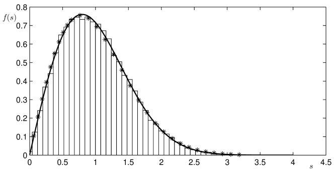
A typical result is shown on the figure 1. The solid line marks the Wigner probability density, (21). Stars show the a the level-spacing probability density for GOE as published in [14], Table A.15.

Figure 1. The odd level spacing distribution of $s_{2j-1}$ for $47$ point interactions with $\alpha=1.001$ and $N=1\cdot 10^{5}$ is compared with the Wigner distribution (solid line) and the exact GOE result (stars).

The dependence of the differences $\Delta F_{W}$ and $\Delta F_{GOE}$ on the parameter $\alpha$ is shown in the figure 2

Figure 2. Plotted are the differences $\Delta F_{W}$ and $\Delta F_{GOE}$ for 24 point interactions and $N=10^{6}$. The dashed horizontal line represents the difference between true GOE and Wigner - (28).

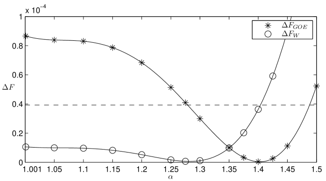
It is not a surprise that for the weak coupling $\alpha\sim 1$ the sequence $s_{2j-1}$ follows the Wigner distribution (21) more closely than Mehta-Gaudin (GOE) distribution. This is just the consequence of the arguments presented in the previous section. It remains true, however, also for $\alpha$ up to $\approx 1.35$ i.e. far outside the weak coupling limit. Even more: there is a distinct minimum of $\Delta F_{W}$ for $\alpha\approx 1.275$. With increasing $\alpha$ the distribution starts,however, approach closer the GOE result then its Wigner approximation. For $\alpha\approx 1.4$ the difference $\Delta F_{GOE}$ displays a clear minimum with $\Delta_{GOE}=3.6457\cdot 10^{-7}$. For this coupling the spacing distribution of the model very close to the true GOE statistic. For $\alpha>1.5$ the agreement however deteriorates step by step. This is understandable since the system with many non-periodically placed interactions is influenced by localization effects for strong enough coupling. For $\alpha\to\infty$ the spectrum becomes a sum of $n$ mutually embedded equidistant sequences and becomes Poissonian for rationally independent points $x_{k}$ - see [15].

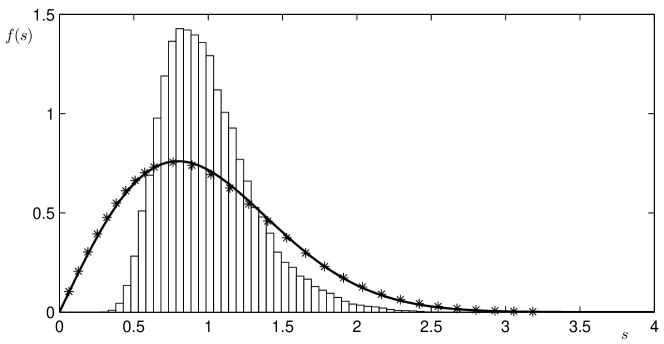
On the other hand the distribution of even spacings $s_{2j}$ never becomes random matrix like, see figure 3.

Figure 3. The even level spacing probability density for $9$ point interactions with $\alpha=1.9$ and $N=1\cdot 10^{5}$ is compared with the Wigner and the GOE distributions.

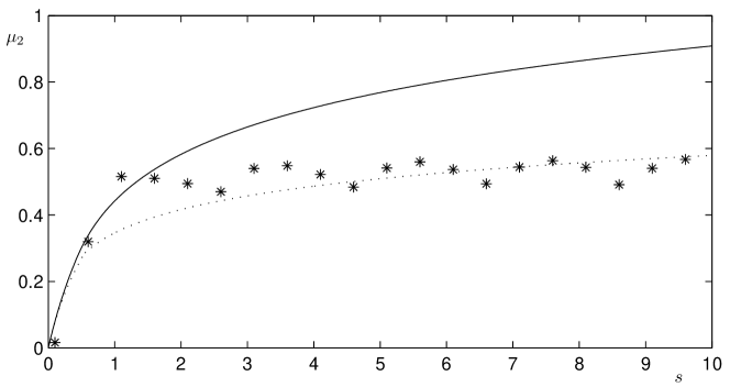
The level spacing statistic depends only on the neighbouring levels. More sensitive statistical properties, like for instance the number variance, describe the correlation of larger level sets. In our case, such large correlations are dominated by the simple geometric structure of the model and by the related periodic orbits (see [16]). This leads finally to oscillatory pattern like the one observed in the number variance and plotted on the figure 4.

Figure 4. The number variance $\mu_{2}=\langle n-\langle n\rangle\rangle^{2}$ evaluated for 24 point interactions with $\alpha=1.4$ and $N=1\cdot 10^{6}$. The solid and dashed curves correspond to the predictions for the Gaussian orthogonal (GOE) and the Gaussian unitary (GUE) ensembles respectively.

The spectral properties of the model are closely related to its topology. Remember that the odd spacings originate from the splitting of the two times degenerate eigenvalues for the free case and are in such a way linked to the fact that the system has a topology of a circle. If we change the topology and replace the periodic boundary condition (2) with the Dirichlet ones $f(0)=f(2\pi)=0$ (i.e. we work on a line segment instead of on a circle) the spacing distribution changes fundamentally and never follows the random matrix theory. In this case the distribution of all spacings (odd and even) is the same. Their common distribution is displayed on the figure 5.

Figure 5. The level spacing distribution of $s_{j}$ for $9$ point interactions on a line segment with $\alpha=1.8$ and $N=1\cdot 10^{5}$ is compared with the Wigner and GOE distributions.

To summarize: we have discussed a simple one dimensional quantum model that displays a level spacing statistics being in a surprising agreement with the predictions of the Gaussian orthogonal ensemble of random matrices. We show that this agreement is related to the topology of the system (circle) and vanishes when the topology is changed (circle is replaced by a line segment).

Acknowledgement: The research was supported by the Ministry of Education, Youth and Sports within the project LC06002 and by the project of the Grant Agency of the Czech Republic No. 202/08/H072. The stimulating discussions with T.Cheon and P.Hejcik are gratefully acknowledged. We also thank to the anonymous referee for valuable remarks.

References

- [1] Bohigas. O, Giannoni, M. J., Schmit, C. Characterization of Chaotic Quantum Spectra and Universality of Level Fluctuation Laws, Phys. Rev. Lett. 52 (1984), 1-4
- [2] Haake, F. Quantum signatures of chaos, Springer, Berlin, 1992
- [3] Hul O., Bauch S., Pakonski P., Savytskyy N., Zyczkowski K., Sirko L. Experimental simulation of quantum graphs by microwave networks, Phys. Rev. E. 69 (2004), 056205
- [4] Kottos, T., Smilansky, U. Periodic Orbit Theory and Spectral Statistics for Quantum Graphs, Annals of Physics 274 (1998), 76-124
- [5] Dabaghian, Yu., Blümel, R. Explicit Spectral formulas for scaling quantum graphs, Phys. Rev. E. 70 (2004), 046206
- [6] Gnutzmann, S., Smilansky, U. Quantum Graphs: Application to Quantum Chaos and Universal Spectral Statistics, Adv. Phys. 55 (2006), 527-625
- [7] Fülöp, T., Tsutsui, I. A Free Particle on a Circle with Point Interaction, Phys. Lett. A 264 (2000), 366-374
- [8] Cheon, T., Fülöp, T., Tsutsui, I. Symmetry, Duality and Anoholonmy of Point Interaction in One Dimension, Annals of Physics 294 (2001), 1-23
- [9] Chernoff, P.R., Hughes, R.J. A New Class of Point Interaction in One Dimension, J. Funct. Anal. 111 (1993), 97-117
- [10] Cheon, T., Shigehara, T. Realizing discontinuous wave functions with renormalized short-range potentials, Phys. Lett. A 243 (1998), 111-116
- [11] Hejčík, P., Cheon, T. Irregular Dynamics in a Solvable One-Dimensional Quantum Graph, Phys. Lett. A 356 (2006), 290-293
- [12] Dunford, N., Schwartz, J. T. Linear operators - Part II, New York: John Wiley & Sons, Inc., 1964
- [13] Kuipers, L., Niederreiter, H. Uniform Distribution of Sequences, New York: John Wiley & Sons, Inc., 1974
- [14] Mehta, M. L. Random matrices, Third Edition, San Diego: Elsevier, 2004
- [15] Casati G., Chirikov B.V., Guarneri I. Energy level statistic of integrable quantum systems Phys. Rev. Lett. 54 (1985), 1350 - 1353
- [16] Berry, M. V. Semiclassical theory of spectral rigidity, Proc. R. Soc. A 400 (1985), 229-251