On the Power of Quantum Encryption Keys

Abstract

The standard definition of quantum state randomization, which is the quantum analog of the classical one-time pad, consists in applying some transformation to the quantum message conditioned on a classical secret key $k$. We investigate encryption schemes in which this transformation is conditioned on a quantum encryption key state $\rho_{\_}k$ instead of a classical string, and extend this symmetric-key scheme to an asymmetric-key model in which copies of the same encryption key $\rho_{\_}k$ may be held by several different people, but maintaining information-theoretical security.

We find bounds on the message size and the number of copies of the encryption key which can be safely created in these two models in terms of the entropy of the decryption key, and show that the optimal bound can be asymptotically reached by a scheme using classical encryption keys.

This means that the use of quantum states as encryption keys does not allow more of these to be created and shared, nor encrypt larger messages, than if these keys are purely classical.

1 Introduction

1.1 Quantum Encryption

To encrypt a quantum state $\sigma$, the standard procedure consists in applying some (unitary) transformation $U_{\_}k$ to the state, which depends on a classical string $k$. This string serves as secret key, and anyone who knows this key can perform the reverse operation and obtain the original state. If the transformations $U_{\_}1,U_{\_}2,\dotsc$ are chosen with probabilities $p_{\_}1,p_{\_}2,\dotsc$, such that when averaged over all possible choices of key,

$$\mathcal{R}(\sigma)=\sum_{\_}kp_{\_}kU_{\_}k\sigma U_{\_}k^{\dagger},$$ (1)

the result looks random, i.e., close to the fully mixed state, $\mathcal{R}(\sigma)\approx\mathbb{I}/d$, this cipher can safely be transmitted on an insecure channel. This procedure is called approximate quantum state randomization or approximate quantum one-time pad [1, 2, 3] or quantum one-time pad, quantum Vernam cipher or quantum private channel in the case of perfect security [4, 5, 6], and is the quantum equivalent of the classical one-time pad.

An encryption scheme which uses such a randomization procedure is called symmetric, because the same key is used to encrypt and decrypt the message. An alternative paradigm is asymmetric-key cryptography, in which a different key is used for encryption and decryption. In such a cryptosystem the encryption key may be shared amongst many different people, because possessing this key is not sufficient to perform the reverse operation, decryption. This can be seen as a natural extension of symmetric-key cryptography, because this latter corresponds to the special case in which the encryption and decryption keys are identical and can be shared with only one person.

Although the encryption model given in Eq. (1) is symmetric, by replacing the classical encryption key with a quantum state we can make it asymmetric. To see this, let us rewrite Eq. (1) as

$$\mathcal{R}(\sigma)=\sum_{\_}kp_{\_}k\operatorname{tr}_{\_}K\left[U\left({\lvert k\rangle\!\langle k\rvert}^{K}\otimes\sigma^{S}\right)U^{\dagger}\right],$$ (2)

where $U:=\sum_{\_}k{\lvert k\rangle\!\langle k\rvert}\otimes U_{\_}k$. The encryption key in Eq. (2), ${\lvert k\rangle\!\langle k\rvert}$, is diagonal in the computational basis, i.e., classical, but an arbitrary quantum state, $\rho_{\_}k$, could be used instead, e.g.,

$$\mathcal{R}(\sigma)=\sum_{\_}kp_{\_}k\operatorname{tr}_{\_}K\left[U\left(\rho_{\_}k^{K}\otimes\sigma^{S}\right)U^{\dagger}\right],$$ (3)

for some set of quantum encryption keys $\{\rho_{\_}k\}_{\_}k$.

If the sender only holds such a quantum encryption key state $\rho_{\_}k$ without knowing the corresponding decryption key $k$, then the resulting model is asymmetric in the sense that possessing this copy of the encryption key state is enough to perform the encryption, but not to decrypt. So many different people can hold copies of the encryption key without compromising the security of the scheme. It is generally impossible to distinguish between non-orthogonal quantum states with certainty (we refer to the textbook by Nielsen and Chuang [7] for an introduction to quantum information), so measuring a quantum state cannot tell us precisely what it is, and possessing a copy of the encryption key state does not allow us to know how the quantum message got transformed, making it impossible to guess the message, except with exponentially small probability.

Up to roughly $\log N$ copies of a state can be needed to discriminate between $N$ possible states [8], so such a scheme could allow the same encryption key to be used several times, if multiple copies of this quantum key state are shared with any party wishing to encrypt a message. The scheme will stay secure as long as the number of copies created stays below a certain threshold. What is more, the security which can be achieved is information-theoretic like for standard quantum state randomization schemes [9], not computational like most asymmetric-key encryption schemes.

Such an asymmetric-key cryptosystem is just a possible application of a quantum state randomization scheme which uses quantum keys. It is also interesting to study quantum state randomization with quantum keys for itself (in the symmetric-key model), without considering other parties holding extra copies of the same encryption key. In this paper we study these schemes in both the symmetric-key and asymmetric-key models, and compare their efficiency in terms of message size and number of usages of the same encryption key to quantum state randomization schemes which use only classical keys.

1.2 Related Work

Quantum one-time pads were first proposed in [4, 5] for perfect security, then approximate security was considered in, e.g., [1, 2, 3]. All these schemes assume the sender and receiver share some secret classical string which is used only once to perform the encryption. We extend these models in the symmetric-key case by conditioning the encryption operation on a quantum key and considering security with multiple uses of the same key, and then in the asymmetric-key case by considering security with multiple users holding copies of the same encryption key.

The first scheme using quantum keys in an asymmetric-key model was proposed by Kawachi et al. [10], although they considered the restricted scenario of classical messages. Their scheme can encrypt a $1$ bit classical message, and their security proof is computational, as it reduces the task of breaking the scheme to a graph automorphism problem. They extended their scheme to a multi-bit version [11], but without security proof. Hayashi et al. [9] then gave an information-theoretical security proof for [11]. The quantum asymmetric-key model we consider is a generalization and extension of that of [10, 11].

1.3 Main Contributions

The main result of this paper is that using quantum encryption keys has no advantage over classical keys with respect to the number of copies of the encryption key which can be safely created and to the size of the messages which can be encrypted, both in the symmetric and asymmetric-key models. Contrary to what was believed and motivated previous works with quantum keys, the intrinsic indistinguishability of quantum states does not allow more of these to be created and shared as encryption keys, than if these keys are purely classical.

To show this, we first find an upper bound on the quantum message size and on the number of copies of the encryption key which can be securely produced. We show that if $t$ copies of the key are created and if the quantum messages encrypted are of dimension $d$, then they have to be such that $t\log d\lesssim\operatorname{H}\left(\mathcal{K}\right)$ for the scheme to be secure, where $\operatorname{H}\left(\mathcal{K}\right)$ is the entropy of the decryption key.

We then construct a quantum state randomization scheme and show that it meets this upper bound in both the symmetric and asymmetric-key models. The encryption keys this scheme uses are however all diagonal in the same bases, i.e., classical. This means that the scheme with classical keys is optimal in terms of message size and number of usages of the same key, and no scheme with quantum keys can perform better.

We also show how to extend quantum asymmetric-key encryption schemes for classical message (such as [11]) to encrypt quantum messages as well. To do this, we combine these schemes for classical messages with a standard quantum one-time pad, and prove that the resulting scheme is still secure.

1.4 Organization of the Paper

In Section 2 we develop the encryption models with quantum keys sketched in this introduction. We first redefine quantum state randomization schemes using quantum keys instead of classical keys in Section 2.1 and generalize the standard security definition for multiple usage of the same key in this symmetric-key model. In Section 2.2 we then show how to construct an asymmetric-key cryptosystem using such a quantum state randomization scheme with quantum keys and define its security. Section 2.3 contains a few notes about the special case of classical messages, which are relevant for the rest of the paper.

In Section 3 we find an upper bound on the message size and number of copies of the encryption key which can be created, both for the symmetric and asymmetric-key models.

In Section 4 we construct a quantum state randomization scheme which uses classical encryption keys, but which meets the optimality bounds for quantum keys from the previous section in both models. We give this construction in three steps. First in Section 4.1 we construct a scheme which can randomize classical messages only. Then in Section 4.2 we show how to combine this scheme for classical messages with a standard approximate quantum one-time pad to randomize any quantum state. And finally in Section 4.3 we calculate the key size of the scheme proposed and show that it corresponds to the bound found in Section 3.

We conclude in Section 5 with a brief summary and further comments about the results.

2 Encryption Model

2.1 Quantum Encryption Keys

Let us consider a setting in which we have two parties, a sender and a receiver, who wish to transmit a quantum state, $\sigma$, from one to the other in a secure way over an insecure channel. If they share a secret classical string, $k$, they can apply some completely positive, trace-preserving (CPTP) map $\mathcal{E}_{\_}k$ to the quantum message and send the cipher $\mathcal{E}_{\_}k(\sigma)$. If the key $k$ was chosen with probability $p_{\_}k$, to any person who does not know this key the transmitted state is

$$\mathcal{R}(\sigma)=\sum_{\_}kp_{\_}k\mathcal{E}_{\_}k(\sigma),$$ (4)

which will look random for “well chosen” maps $\mathcal{E}_{\_}k$. This is the most general from of quantum state randomization [6].

If instead the sender has a quantum state $\rho_{\_}k$, he can apply some CPTP map $\mathcal{E}$ to both the shared state and the quantum message, and send $\mathcal{E}(\rho_{\_}k\otimes\sigma)$. So for someone who does not know $\rho_{\_}k$ the state sent is

$$\mathcal{R}(\sigma)=\sum_{\_}kp_{\_}k\mathcal{E}(\rho_{\_}k\otimes\sigma).$$ (5)

It is clear that Eqs. (4) and (5) produce equivalent ciphers, because for every set of CPTP maps $\{\mathcal{E}_{\_}k\}_{\_}k$ there exists a map $\mathcal{E}$ and set of states $\{\rho_{\_}k\}_{\_}k$ such that for all messages $\sigma$, $\mathcal{E}_{\_}k(\sigma)=\mathcal{E}(\rho_{\_}k\otimes\sigma)$, and vice versa. The difference lies in the knowledge needed to perform the encryption. In the first case (Eq. (4)) the sender needs to know the secret key $k$ to know which CPTP map $\mathcal{E}_{\_}k$ to apply. In the second case (Eq. (5)) the sender only needs to hold a copy of the encryption key $\rho_{\_}k$, he does not need to know what it is or what secret key $k$ it corresponds to. This allows us to construct in Section 2.2 a quantum asymmetric-key cryptosystem in which copies of the same encryption key $\rho_{\_}k$ can be used by many different users. In this section we focus on the symmetric-key model and define quantum state randomization (QSR) schemes with quantum encryption keys and their security in this model.

Definition 1.

Let $\mathcal{B}(\mathcal{H})$ denote the set of linear operators on $\mathcal{H}$.

A quantum state randomization (QSR) scheme with quantum encryption keys consists of the following tuple,

$$\mathbb{T}=\left(P_{\_}\mathcal{K},\{\rho_{\_}k\}_{\_}{k\in\mathcal{K}},\mathcal{E}\right).$$

$\rho_{\_}k\in\mathcal{B}(\mathcal{H}_{\_}K)$ are density operators on a Hilbert space $\mathcal{H}_{\_}K$. They are called encryption keys and are indexed by elements $k\in\mathcal{K}$ called decryption keys.

$P_{\_}\mathcal{K}(\cdot)$ is a probability distribution over the set of decryption keys $\mathcal{K}$, corresponding to the probability with which each en/decryption key-pair should be chosen.

$\mathcal{E}:\mathcal{B}(\mathcal{H}_{\_}K\otimes\mathcal{H}_{\_}S)\rightarrow\mathcal{B}(\mathcal{H}_{\_}C)$, is a completely positive, trace-preserving (CPTP) map from the set of linear operators on the joint system of encryption key and message Hilbert spaces, $\mathcal{H}_{\_}K$ and $\mathcal{H}_{\_}S$ respectively, to the set of linear operators on the cipher Hilbert space $\mathcal{H}_{\_}C$, and is called encryption operator.

To encrypt a quantum message given by its density operator $\sigma\in\mathcal{B}(\mathcal{H}_{\_}S)$ with the encryption key $\rho_{\_}k$, the encryption operator is applied to the key and message, resulting in the cipher

$$\rho_{\_}{k,\sigma}:=\mathcal{E}(\rho_{\_}k\otimes\sigma).$$

Definition 1 describes how to encrypt a quantum message, but for such a scheme to be useful, it must also be possible to decrypt the message for someone who knows which key $k$ was used, i.e., it must be possible to invert the encryption operation.

Definition 2.

A QSR scheme given by the tuple $\mathbb{T}=\left(P_{\_}\mathcal{K},\{\rho_{\_}k\}_{\_}{k\in\mathcal{K}},\mathcal{E}\right)$ is said to be invertible on the set $\mathcal{S}\subseteq\mathcal{B}(\mathcal{H}_{\_}S)$ if for every $k\in\mathcal{K}$ with $P_{\_}{\mathcal{K}}(k)>0$ there exists a CPTP map $\mathcal{D}_{\_}k:\mathcal{B}(\mathcal{H}_{\_}C)\rightarrow\mathcal{B}(\mathcal{H}_{\_}S)$ such that for all density operators $\sigma\in\mathcal{S}$,

$$\mathcal{D}_{\_}k\mathcal{E}(\rho_{\_}k\otimes\sigma)=\sigma.$$

Furthermore, a QSR scheme must – as its name says – randomize a quantum state. We define this in the same way as previous works on approximate quantum state randomization [1, 2, 3], by bounding the distance between the ciphers averaged over all possible choices of key and some state independent from the message. We however generalize this to encrypt $t$ messages with the same key, because the asymmetric-key model we define Section 2.2 will need this. It is always possible to consider the case $t=1$ in the symmetric-key model, if multiple uses of the same key are not desired.

We will use the trace norm as distance measure between two states, because it is directly related to the probability that an optimal measurement can distinguish between these two states, and is therefore meaningful in the context of eavesdropping. The trace norm of a matrix $A$ is defined by ${\|A\|_{\text{tr}}}:=\operatorname{tr}{|A|}=\operatorname{tr}{\sqrt{A^{\dagger}A}}$, which is also equal to the sum of the singular values of $A$.

Definition 3.

A QSR scheme given by the tuple $\mathbb{T}=\left(P_{\_}\mathcal{K},\{\rho_{\_}k\}_{\_}{k\in\mathcal{K}},\mathcal{E}\right)$ is said to be $(t,\epsilon)$-randomizing on the set $\mathcal{S}\subseteq\mathcal{B}(\mathcal{H}_{\_}S)$ if there exists a density operator $\tau\in\mathcal{B}\left(\mathcal{H}_{\_}C^{\otimes t}\right)$ such that for all $t$-tuples of message density operators $\omega=(\sigma_{\_}1,\dotsc,\sigma_{\_}t)\in\mathcal{S}^{\times t}$

$${\|\mathcal{R}(\omega)-\tau\|_{\text{tr}}}\leq\epsilon,$$ (6)

where $\mathcal{R}(\omega)=\sum_{\_}kP_{\_}\mathcal{K}(k)\rho_{\_}{k,\sigma_{\_}1}\otimes\dotsb\otimes\rho_{\_}{k,\sigma_{\_}t}$ and $\rho_{\_}{k,\sigma_{\_}i}=\mathcal{E}(\rho_{\_}k\otimes\sigma_{\_}i)$.

2.2 Quantum Asymmetric-Key Cryptosystem

As announced in the previous section, the idea behind the quantum asymmetric-key cryptosystem model is that many different people hold a copy of some quantum state $\rho_{\_}k$ which serves as encryption key, and anyone who wishes to send a message to the originator of the encryption keys uses a quantum state randomization scheme, as described in Definition 1. This is depicted in Figure 1.

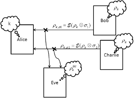
Figure 1: Quantum asymmetric-key cryptosystem model. Bob and Charlie hold copies of Alice’s encryption key $\rho_{\_}k$. To send her a message, they encrypt it with the key and a given QSR scheme, and send the resulting cipher to her. An eavesdropper, Eve, may intercept the ciphers as well as possess some copies of the encryption key herself.

If the QSR scheme used to encrypt the messages is $(t,\epsilon)$-randomizing and no more than $t$ copies of the encryption key were released, an eavesdropper who intercepts the ciphers will not be able to distinguish them from some state independent from the messages, so not get any information about these messages. This is however not the only attack he may perform.

As we consider a scenario in which copies of the encryption key are shared between many different people, the adversary could hold one or many of them. If a total of $t$ copies of the encryption key were produced and $t_{\_}1$ were used to encrypt messages $\omega=(\sigma_{\_}1,\dotsc,\sigma_{\_}{t_{\_}1})$, in the worst case we have to assume that the adversary has the $t_{\_}2:=t-t_{\_}1$ remaining unused copies of the key. So his total state is

$$\rho^{E}_{\_}\omega:=\sum_{\_}{k\in\mathcal{K}}P_{\_}{\mathcal{K}}(k)\rho_{\_}{k,\sigma_{\_}1}\otimes\dotsb\otimes\rho_{\_}{k,\sigma_{\_}{t_{\_}1}}\otimes\rho_{\_}k^{\otimes t_{\_}2},$$ (7)

where $\rho_{\_}{k,\sigma_{\_}i}$ is the cipher of the message $\sigma_{\_}i$ encrypted with the key $\rho_{\_}k$. This leads to the following security definition.

Definition 4.

We call a quantum asymmetric-key cryptosystem $(t,\epsilon)$-indistinguishable on the set $\mathcal{S}\subseteq\mathcal{B}(\mathcal{H}_{\_}S)$ if for all $t_{\_}1\in\{0,1,\dotsc,t\}$, $t_{\_}2:=t-t_{\_}1$, there exists a density operator $\tau\in\mathcal{B}\left(\mathcal{H}_{\_}C^{\otimes t_{\_}1}\otimes\mathcal{H}_{\_}K^{\otimes t_{\_}2}\right)$ such that for all $t_{\_}1$-tuples of message density operators $\omega=(\sigma_{\_}1,\dotsc,\sigma_{\_}{t_{\_}1})\in\mathcal{S}^{\times t_{\_}1}$,

$${\|\rho^{E}_{\_}\omega-\tau\|_{\text{tr}}}\leq\epsilon,$$

where $\rho^{E}_{\_}\omega$ is the state the adversary obtains as defined in Eq. (7).

Remark 5.

Definition 4 is clearly more general than the security criteria of Definition 3 ($(t,\epsilon)$-randomization) as this latter corresponds to the special case $t_{\_}1=t$. However, for the scheme constructed in Section 4 the two are equivalent, and proving one proves the other. This is the case in particular if the encryption key is equal to the cipher of some specific message $\sigma_{\_}0$, i.e., $\rho_{\_}k=\rho_{\_}{k,\sigma_{\_}0}=\mathcal{E}(\rho_{\_}k\otimes\sigma_{\_}0)$, in which case holding an extra copy of the encryption key does not give more information about the decryption key than holding an extra cipher state.

2.3 Classical Messages

In the following sections we will also be interested in the special case of schemes which encrypt classical messages only. Classical messages can be represented by a set of mutually orthogonal quantum states, which we will take to be the basis states of the message Hilbert space and denote by $\{{\lvert s\rangle}\}_{\_}{s\in\mathcal{S}}$. So these schemes must be invertible and randomizing on the set of basis states of the message Hilbert space.

When considering classical messages only, we will simplify the notation when possible and represent a message by a string $s$ instead of by its density matrix ${\lvert s\rangle\!\langle s\rvert}$, e.g., the cipher of the message $s$ encrypted with the key $\rho_{\_}k$ is

$$\rho_{\_}{k,s}:=\mathcal{E}\left(\rho_{\_}k\otimes{\lvert s\rangle\!\langle s\rvert}\right).$$

Remark 6.

Definition 2 (invertibility) can be simplified when only classical messages are considered: a QSR scheme given by the tuple $\mathbb{T}=\left(P_{\_}\mathcal{K},\{\rho_{\_}k\}_{\_}{k\in\mathcal{K}},\mathcal{E}\right)$ is invertible for the set of classical messages $\mathcal{S}$, if for every $k\in\mathcal{K}$ with $P_{\_}{\mathcal{K}}(k)>0$ the ciphers $\{\rho_{\_}{k,s}\}_{\_}{s\in\mathcal{S}}$ are mutually orthogonal, where $\rho_{\_}{k,s}:=\mathcal{E}\left(\rho_{\_}k\otimes{\lvert s\rangle\!\langle s\rvert}\right)$ for some orthonormal basis $\{{\lvert s\rangle}\}_{\_}{s\in\mathcal{S}}$ of the message Hilbert space $\mathcal{H}_{\_}S$.

We will also use a different but equivalent definition to measure how well a scheme can randomize a message when dealing with classical messages. This new security criteria allows us to simplify some proofs.

Definition 7.

A QSR scheme given by the tuple $\mathbb{T}=\left(P_{\_}\mathcal{K},\{\rho_{\_}k\}_{\_}{k\in\mathcal{K}},\mathcal{E}\right)$ is said to be $(t,\epsilon)$-secure for the set of classical messages $\mathcal{S}$ if for all probability distributions $P_{\_}{\mathcal{S}^{t}}(\cdot)$ over the set of $t$-tuples of messages $\mathcal{S}^{\times t}$,

$${\|\rho^{S^{t}C^{t}}-\rho^{S^{t}}\otimes\rho^{C^{t}}\|_{\text{tr}}}\leq\epsilon,$$ (8)

where $\rho^{S^{t}C^{t}}$ is the state of the joint systems of $t$-fold message and cipher Hilbert spaces, and $\rho^{S^{t}}$ and $\rho^{C^{t}}$ are the result of tracing out the cipher respectively message systems. I.e.,

$$\rho^{S^{t}C^{t}} =\sum_{\_}{s\in\mathcal{S}^{\times t}}P_{\_}{\mathcal{S}^{t}}(s){\lvert s\rangle\!\langle s\rvert}\otimes\sum_{\_}{k\in\mathcal{K}}P_{\_}{\mathcal{K}}(k)\rho_{\_}{k,s_{\_}1}\otimes\dotsb\otimes\rho_{\_}{k,s_{\_}t},$$

$$\rho^{S^{t}} =\sum_{\_}{s\in\mathcal{S}^{\times t}}P_{\_}{\mathcal{S}^{t}}(s){\lvert s\rangle\!\langle s\rvert},$$

$$\rho^{C^{t}} =\sum_{\_}{s\in\mathcal{S}^{\times t}}P_{\_}{\mathcal{S}^{t}}(s)\sum_{\_}{k\in\mathcal{K}}P_{\_}{\mathcal{K}}(k)\rho_{\_}{k,s_{\_}1}\otimes\dotsb\otimes\rho_{\_}{k,s_{\_}t},$$

where $s=(s_{\_}1,\dotsc,s_{\_}t)$.

This security definition can be interpreted the following way. No matter what the probability distribution on the secret messages is – let the adversary choose it – the message and cipher spaces are nearly in product form, i.e., the cipher gives next to no information about the message.

The following lemma proves that this new security definition is equivalent to the previous one (Definition 3) up to a constant factor.

Lemma 8.

If a QSR scheme is $(t,\epsilon)$-randomizing for a set of classical messages $\mathcal{S}$, then it is $(t,2\epsilon)$-secure for $\mathcal{S}$. If a QSR scheme is $(t,\epsilon)$-secure for a set of classical messages $\mathcal{S}$, then it is $(t,2\epsilon)$-randomizing for $\mathcal{S}$.

Proof.

In order to simplify the notation we will set $s:=(s_{\_}1,\dotsc,s_{\_}t)$ and $\rho_{\_}{k,s}:=\rho_{\_}{k,s_{\_}1}\otimes\dotsb\otimes\rho_{\_}{k,s_{\_}t}$. The left-hand side of Eq. (8) can then be rewritten as

$${\|\rho^{S^{t}C^{t}}-\rho^{S^{t}}\otimes\rho^{C^{t}}\|_{\text{tr}}}$$

$$\qquad=\left\|\sum_{\_}{s\in\mathcal{S}^{\times t}}P_{\_}{\mathcal{S}^{t}}(s){\lvert s\rangle\!\langle s\rvert}\otimes\sum_{\_}{k\in\mathcal{K}}P_{\_}{\mathcal{K}}(k)\rho_{\_}{k,s}\right.$$

$$\qquad\qquad-\left.\sum_{\_}{s\in\mathcal{S}^{\times t}}P_{\_}{\mathcal{S}^{t}}(s){\lvert s\rangle\!\langle s\rvert}\otimes\sum_{\_}{\begin{subarray}{c}r\in\mathcal{S}^{\times t}\\ k\in\mathcal{K}\end{subarray}}P_{\_}{\mathcal{K}}(k)P_{\_}{\mathcal{S}^{t}}(r)\rho_{\_}{k,r}\right\|_{\_}\text{tr}$$

$$\qquad=\sum_{\_}{s\in\mathcal{S}^{\times t}}P_{\_}{\mathcal{S}^{t}}(s){\|\sum_{\_}{k\in\mathcal{K}}P_{\_}{\mathcal{K}}(k)\rho_{\_}{k,s}-\sum_{\_}{\begin{subarray}{c}r\in\mathcal{S}^{\times t}\\ k\in\mathcal{K}\end{subarray}}P_{\_}{\mathcal{K}}(k)P_{\_}{\mathcal{S}^{t}}(r)\rho_{\_}{k,r}\|_{\text{tr}}}.$$ (9)

If this must be less than $\epsilon$ for all probability distributions $P_{\_}{\mathcal{S}^{t}}$ then for the distribution $P_{\_}{\mathcal{S}^{t}}(s_{\_}1)=P_{\_}{\mathcal{S}^{t}}(s_{\_}2)=1/2$ for any two elements $s_{\_}1,s_{\_}2\in\mathcal{S}^{\times t}$ we have from Eq. (9)

$$\frac{1}{2}{\|\sum_{\_}{k\in\mathcal{K}}P_{\_}{\mathcal{K}}(k)\rho_{\_}{k,s_{\_}1}-\sum_{\_}{k\in\mathcal{K}}P_{\_}{\mathcal{K}}(k)\rho_{\_}{k,s_{\_}2}\|_{\text{tr}}}\leq\epsilon.$$

This immediately implies $(t,2\epsilon)$-randomization.

To prove the converse we apply the triangle inequality to Eq. (9) and get

$${\|\rho^{S^{t}C^{t}}-\rho^{S^{t}}\otimes\rho^{C^{t}}\|_{\text{tr}}}\leq\\ \sum_{\_}{s\in\mathcal{S}^{\times t}}P_{\_}{\mathcal{S}^{t}}(s)\sum_{\_}{r\in\mathcal{S}^{\times t}}P_{\_}{\mathcal{S}^{t}}(r){\|\sum_{\_}{k\in\mathcal{K}}P_{\_}{\mathcal{K}}(k)\rho_{\_}{k,s}-\sum_{\_}{k\in\mathcal{K}}P_{\_}{\mathcal{K}}(k)\rho_{\_}{k,r}\|_{\text{tr}}}.$$

By the definition of $(t,\epsilon)$-randomization (Definition 3) and the triangle inequality we know that

$${\|\sum_{\_}{k\in\mathcal{K}}P_{\_}{\mathcal{K}}(k)\rho_{\_}{k,s}-\sum_{\_}{k\in\mathcal{K}}P_{\_}{\mathcal{K}}(k)\rho_{\_}{k,r}\|_{\text{tr}}}\leq 2\epsilon,$$

for all $r,s\in\mathcal{S}^{\times t}$, which concludes the proof. ∎

3 Lower bounds on the Key Size

It is intuitively clear that the more copies of the encryption key state $\rho_{\_}k$ are created, the more information the adversary gets about the decryption key $k\in\mathcal{K}$ and the more insecure the scheme becomes. As it turns out, the number of copies of the encryption key which can be safely used is directly linked to the size of the decryption key, i.e., the cardinality of the decryption key set $\mathcal{K}$.

Let us assume a QSR scheme with quantum encryption keys is used to encrypt classical messages of size $m$. Then if $t$ copies of the encryption key state are released and used, the size of the total message encrypted with the same decryption key $k$ is $tm$. We prove in this section that the decryption key has to be of the same size as the total message to achieve information-theoretical security, i.e., $\log|\mathcal{K}|\gtrsim tm$. In Section 4 we then give a scheme which reaches this bound asymptotically.

Theorem 9.

If a QSR scheme given by the tuple $\mathbb{T}=\left(P_{\_}\mathcal{K},\{\rho_{\_}k\}_{\_}{k\in\mathcal{K}},\mathcal{E}\right)$ is invertible for the set of classical messages $\mathcal{S}$, then when $t$ messages $(s_{\_}1,\dotsc,s_{\_}t)$ are chosen from $\mathcal{S}$ with (joint) probability distribution $P_{\_}{\mathcal{S}^{t}}(s_{\_}1,\dotsc,s_{\_}t)$ and encrypted with the same key,

$${\|\rho^{S^{t}C^{t}}-\rho^{S^{t}}\otimes\rho^{C^{t}}\|_{\text{tr}}}\geq\frac{\operatorname{H}\left(\mathcal{S}^{t}\right)-\operatorname{H}\left(\mathcal{K}\right)-2}{4t\log|S|},$$ (10)

where $\operatorname{H}(\cdot)$ is the Shannon entropy and $\rho^{S^{t}C^{t}}$ is the state of the $t$-fold message and cipher systems:

$$\begin{split}\rho^{S^{t}C^{t}}&=\sum_{\_}{s\in\mathcal{S}^{\times t}}P_{\_}{\mathcal{S}^{t}}(s){\lvert s\rangle\!\langle s\rvert}\otimes\sum_{\_}{k\in\mathcal{K}}P_{\_}{\mathcal{K}}(k)\rho_{\_}{k,s_{\_}1}\otimes\dotsb\otimes\rho_{\_}{k,s_{\_}t},\\ \rho^{S^{t}}&=\sum_{\_}{s\in\mathcal{S}^{\times t}}P_{\_}{\mathcal{S}^{t}}(s){\lvert s\rangle\!\langle s\rvert},\\ \rho^{C^{t}}&=\sum_{\_}{s\in\mathcal{S}^{\times t}}P_{\_}{\mathcal{S}^{t}}(s)\sum_{\_}{k\in\mathcal{K}}P_{\_}{\mathcal{K}}(k)\rho_{\_}{k,s_{\_}1}\otimes\dotsb\otimes\rho_{\_}{k,s_{\_}t},\end{split}$$ (11)

where $s=(s_{\_}1,\dotsc,s_{\_}t)$.

Proof.

A theorem by Alicki and Fanes [12] tells us that for any two states $\rho^{AB}$ and $\sigma^{AB}$ on the joint system $\mathcal{H}_{\_}{AB}=\mathcal{H}_{\_}A\otimes\mathcal{H}_{\_}B$ with $\delta:={\|\rho^{AB}-\sigma^{AB}\|_{\text{tr}}}\leq 1$ and $d_{\_}A:=\dim\mathcal{H}_{\_}A$,

$$\left|\operatorname{S}\left(\rho^{AB}\middle|\rho^{B}\right)-\operatorname{S}\left(\sigma^{AB}\middle|\sigma^{B}\right)\right|\leq 4\delta\log d_{\_}A+2h\left(\delta\right),$$ (12)

where $\operatorname{S}\left(\rho^{AB}\middle|\rho^{B}\right):=\operatorname{S}\left(\rho^{AB}\right)-\operatorname{S}\left(\rho^{B}\right)$ is the conditional Von Neumann entropy and $h(p):=p\log\frac{1}{p}+(1-p)\log\frac{1}{1-p}$ is the binary entropy. $h(\delta)\leq 1$, so from Eq. (12) we get

$${\|\rho^{AB}-\sigma^{AB}\|_{\text{tr}}}\geq\frac{\left|\operatorname{S}\left(\rho^{AB}\middle|\rho^{B}\right)-\operatorname{S}\left(\sigma^{AB}\middle|\sigma^{B}\right)\right|-2}{4\log d_{\_}A}.$$

By applying this to the left-hand side of Eq. (10) we obtain

$${\|\rho^{S^{t}C^{t}}-\rho^{S^{t}}\otimes\rho^{C^{t}}\|_{\text{tr}}}\geq\frac{\operatorname{S}\left(\rho^{S^{t}}\right)+\operatorname{S}\left(\rho^{C^{t}}\right)-\operatorname{S}\left(\rho^{S^{t}C^{t}}\right)-2}{4t\log|\mathcal{S}|}.$$

To prove this theorem it remains to show that

$$\operatorname{S}\left(\rho^{S^{t}}\right)+\operatorname{S}\left(\rho^{C^{t}}\right)-\operatorname{S}\left(\rho^{S^{t}C^{t}}\right)\geq\operatorname{H}\left(\mathcal{S}^{t}\right)-\operatorname{H}\left(\mathcal{K}\right).$$

For this we will need the two following bounds on the Von Neumann entropy (see e.g, [7]):

$$\operatorname{S}\left(\sum_{\_}{x\in\mathcal{X}}p_{\_}x\rho_{\_}x\right) \geq\sum_{\_}{x\in\mathcal{X}}p_{\_}x\operatorname{S}\left(\rho_{\_}x\right),$$

$$\operatorname{S}\left(\sum_{\_}{x\in\mathcal{X}}p_{\_}x\rho_{\_}x\right) \leq\operatorname{H}\left(\mathcal{X}\right)+\sum_{\_}{x\in\mathcal{X}}p_{\_}x\operatorname{S}\left(\rho_{\_}x\right).$$

Equality is obtained in the second equation if the states $\{\rho_{\_}x\}_{\_}{x\in\mathcal{X}}$ are all mutually orthogonal. By using these bounds and Eq. (11) we see that

$$\operatorname{S}\left(\rho^{S^{t}C^{t}}\right) =\operatorname{H}\left(\mathcal{S}^{t}\right)+\sum_{\_}{s\in\mathcal{S}^{\times t}}P_{\_}{\mathcal{S}^{t}}(s)\operatorname{S}\left(\sum_{\_}{k\in\mathcal{K}}P_{\_}{\mathcal{K}}(k)\rho_{\_}{k,s_{\_}1}\otimes\dotsb\otimes\rho_{\_}{k,s_{\_}t}\right)$$

$$\leq\operatorname{H}\left(\mathcal{S}^{t}\right)+\operatorname{H}\left(\mathcal{K}\right)+\sum_{\_}{\begin{subarray}{c}s\in\mathcal{S}^{\times t}\\ k\in\mathcal{K}\end{subarray}}P_{\_}{\mathcal{K}}(k)P_{\_}{\mathcal{S}^{t}}(s)\operatorname{S}\left(\rho_{\_}{k,s_{\_}1}\otimes\dotsb\otimes\rho_{\_}{k,s_{\_}t}\right),$$

$$\operatorname{S}\left(\rho^{S^{t}}\right) =\operatorname{H}\left(\mathcal{S}^{t}\right),$$

$$\operatorname{S}\left(\rho^{C^{t}}\right) \geq\sum_{\_}{k\in\mathcal{K}}P_{\_}{\mathcal{K}}(k)\operatorname{S}\left(\sum_{\_}{s\in\mathcal{S}^{\times t}}P_{\_}{\mathcal{S}^{t}}(s)\rho_{\_}{k,s_{\_}1}\otimes\dotsb\otimes\rho_{\_}{k,s_{\_}t}\right)$$

$$=\operatorname{H}\left(\mathcal{S}^{t}\right)+\sum_{\_}{\begin{subarray}{c}s\in\mathcal{S}^{\times t}\\ k\in\mathcal{K}\end{subarray}}P_{\_}{\mathcal{K}}(k)P_{\_}{\mathcal{S}^{t}}(s)\operatorname{S}\left(\rho_{\_}{k,s_{\_}1}\otimes\dotsb\otimes\rho_{\_}{k,s_{\_}t}\right).$$

We have equality in the last line because the scheme is invertible on $\mathcal{S}$, i.e., by Definition 2 and Remark 6 the states $\{\rho_{\_}{k,s_{\_}1}\otimes\dotsb\otimes\rho_{\_}{k,s_{\_}t}\}_{\_}{s_{\_}1,\dotsc,s_{\_}t\in\mathcal{S}}$ are mutually orthogonal. By putting this all together we conclude the proof. ∎

Corollary 10.

For a QSR scheme to be $(t,\epsilon)$-randomizing or $(t,\epsilon)$-indistinguishable, it is necessary that

$$\operatorname{H}\left(\mathcal{K}\right)\geq(1-8\epsilon)t\log d-2,$$ (13)

where $d$ is the dimension of the message Hilbert space $\mathcal{H}_{\_}S$ and $\operatorname{H}\left(\mathcal{K}\right)$ is the entropy of the decryption key.

Proof.

Definition 7 says that for a scheme to be $(t,\epsilon)$-secure we need

$${\|\rho^{S^{t}C^{t}}-\rho^{S^{t}}\otimes\rho^{C^{t}}\|_{\text{tr}}}\leq\epsilon$$

for all probability distributions $P_{\_}{\mathcal{S}^{t}}$. So for the uniform distribution we get from Theorem 9 that for a scheme to be $(t,\epsilon)$-secure we need

$$\operatorname{H}\left(\mathcal{K}\right)\geq(1-4\epsilon)t\log|\mathcal{S}|-2.$$

By Lemma 8 we then have the condition

$$\operatorname{H}\left(\mathcal{K}\right)\geq(1-8\epsilon)t\log|\mathcal{S}|-2$$

for the scheme to be $(t,\epsilon)$-randomizing for the classical messages $\mathcal{S}$. And as classical messages are a subset of quantum messages – namely an orthonormal basis of the message Hilbert space – this bound extends to the case of quantum messages on a Hilbert space of dimension $d_{\_}S=|\mathcal{S}|$.

As $(t,\epsilon)$-randomization is a special case of $(t,\epsilon)$-indistinguishability, namely for $t_{\_}1=t$, it is immediate that this lower bound also applies to $(t,\epsilon)$-indistinguishability. ∎

Remark 11.

Approximate quantum one-time pad schemes usually only consider the special case in which the cipher has the same dimension as the message [1, 3]. A more general scenario in which an ancilla is appended to the message is however also possible. It was proven in [6] that for perfect security such an extended scheme needs a key of the same size as in the restricted scenario, namely $2\log d$. Corollary 10 for $t=1$ shows the same for approximate security, namely roughly $\log d$ bits of key are necessary, just as when no ancilla is present.

4 Near-Optimal Scheme

To simplify the presentation of the QSR scheme, we first define it for classical messages in Section 4.1, show that it is invertible and find a bound on $t$, the number of copies of the encryption key which can be released, for it to be $(t,\epsilon)$-randomizing for an exponentially small $\epsilon$. In Section 4.2 we extend the scheme to encrypt any quantum message of a given size, and show again that it is invertible and randomizing. And finally in Section 4.3 we calculate the size of the key necessary to encrypt a message of a given length, and show that it is nearly asymptotically equal to the lower bound found in Section 3.

4.1 Classical Messages

Without loss of generality, let the message space be of dimension $\dim\mathcal{H}_{\_}S=2^{m}$. The classical messages can then be represented by strings of length $m$, $\mathcal{S}:=\{0,1\}^{m}$. We now define a QSR scheme which uses encryption key states of dimension $\dim\mathcal{H}_{\_}K=2^{m+n}$, where $n$ is a security parameter, i.e., the scheme will be $(t,\epsilon)$-randomizing for $\epsilon=2^{-\Theta(n)}$.

We define the set of decryption keys to be the set of all $(m\times n)$ binary matrices,

$$\mathcal{K}:=\{0,1\}^{m\times n}.$$ (14)

This set has size $|\mathcal{K}|=2^{mn}$ and each key is chosen with uniform probability.

For every decryption key $A\in\mathcal{K}$ the corresponding encryption key is defined as

$$\rho_{\_}A:=\frac{1}{2^{n}}\sum_{\_}{x\in\{0,1\}^{n}}{\lvert Ax,x\rangle\!\langle Ax,x\rvert},$$ (15)

where $Ax$ is the multiplication of the matrix $A$ with the vector $x$.

The encryption operator $\mathcal{E}:\mathcal{B}(\mathcal{H}_{\_}K\otimes\mathcal{H}_{\_}S)\rightarrow\mathcal{B}(\mathcal{H}_{\_}C)$ consists in applying the unitary

$$U:=\sum_{\_}{\begin{subarray}{c}x\in\{0,1\}^{n}\\ s,y\in\{0,1\}^{m}\end{subarray}}{\lvert y\oplus s,x\rangle}{\langle y,x\rvert}^{K}{\lvert s\rangle\!\langle s\rvert}^{S}$$

and tracing out the message system $S$, i.e.,

$$\rho_{\_}{A,s}:=\operatorname{tr}_{S}(U\left(\rho_{\_}k^{K}\otimes{\lvert s\rangle\!\langle s\rvert}^{S}\right)U^{\dagger}).$$

This results in the cipher for the message $s$ being

$$\rho_{\_}{A,s}=\frac{1}{2^{n}}\sum_{\_}{x\in\{0,1\}^{n}}{\lvert Ax\oplus s,x\rangle\!\langle Ax\oplus s,x\rvert}.$$ (16)

These states are mutually orthogonal for different messages $s$ so by Remark 6 this scheme is invertible.

We now show that this scheme is $(t,\epsilon)$-randomizing for $\epsilon=2^{-\delta n+1}$ and $t=(1-\delta)n$, $0<\delta<1$.

Theorem 12.

For the QSR scheme defined above in Eqs. (14), (15) and (16) there exists a density operator $\tau\in\mathcal{B}(\mathcal{H}_{\_}C^{\otimes t})$ such that for all $t$-tuples of messages $s=(s_{\_}1,\dotsc,s_{\_}t)\in\mathcal{S}^{\times t}$, if $t=(1-\delta)n$, $0<\delta<1$, then

$${\|\gamma_{\_}s-\tau\|_{\text{tr}}}\leq 2^{-\delta n+1},$$

where $\gamma_{\_}s$ is the encryption of $s$ with this scheme averaged over all possible keys, i.e.,

$$\gamma_{\_}s=\sum_{\_}{A\in\mathcal{K}}P_{\_}{\mathcal{K}}(A)\rho_{\_}{A,s_{\_}1}\otimes\dotsb\otimes\rho_{\_}{A,s_{\_}t}.$$ (17)

Proof.

The $\tau$ in question is the fully mixed state $\tau=\frac{1}{2^{t(m+n)}}\mathbb{I}$. By placing the values of the ciphers from Eq. (16) in Eq. (17) we get

$$\gamma_{\_}s=\frac{1}{2^{mn}2^{tn}}\sum_{\_}{\begin{subarray}{c}A\in\{0,1\}^{m\times n}\\ x_{\_}1,\dotsc,x_{\_}t\in\{0,1\}^{n}\end{subarray}}{\lvert\dotsc,Ax_{\_}i\oplus s_{\_}i,x_{\_}i,\dotsc\rangle\!\langle\dotsc,Ax_{\_}i\oplus s_{\_}i,x_{\_}i,\dotsc\rvert}.$$

A unitary performing bit flips can take $\gamma_{\_}s$ to $\gamma_{\_}r$ for any $s,r\in\mathcal{S}^{t}$, so

$${\|\gamma_{\_}s-\frac{1}{2^{t(m+n)}}\mathbb{I}\|_{\text{tr}}}={\|\gamma_{\_}r-\frac{1}{2^{t(m+n)}}\mathbb{I}\|_{\text{tr}}},$$

and it is sufficient to evaluate

$${\|\gamma_{\_}0-\frac{1}{2^{t(m+n)}}\mathbb{I}\|_{\text{tr}}}=\sum_{\_}{e\in\text{EVec}(\gamma_{\_}0)}\left|w_{\_}e-\frac{1}{2^{t(n+m)}}\right|,$$ (18)

where $e$ are the eigenvectors of $\gamma_{\_}0$ and $w_{\_}e$ the corresponding eigenvalues.

So we need to calculate the eigenvalues of

$$\gamma_{\_}0=\frac{1}{2^{mn}2^{tn}}\sum_{\_}{\begin{subarray}{c}A\in\{0,1\}^{m\times n}\\ x_{\_}1,\dotsc,x_{\_}t\in\{0,1\}^{n}\end{subarray}}{\lvert Ax_{\_}1,x_{\_}1,\dotsc,Ax_{\_}t,x_{\_}t\rangle\!\langle Ax_{\_}1,x_{\_}1,\dotsc,Ax_{\_}t,x_{\_}t\rvert}.$$ (19)

Let us fix $x_{\_}1,\dotsc,x_{\_}t$. It is immediate from the linearity of $Ax$ that if exactly $d$ of the vectors $\{x_{\_}i\}_{\_}{i=1}^{t}$ are linearly independent, then

$$\sum_{\_}{A\in\{0,1\}^{m\times n}}{\lvert Ax_{\_}1,x_{\_}1,\dotsc,Ax_{\_}t,x_{\_}t\rangle\!\langle Ax_{\_}1,x_{\_}1,\dotsc,Ax_{\_}t,x_{\_}t\rvert}$$

uniformly spans a space of dimension $2^{dm}$, and for different values of $x_{\_}1,\dotsc,x_{\_}t$ these subspaces are all mutually orthogonal. Let $D_{\_}t$ be the random variable representing the number of independent vectors amongst $t$ binary vectors of length $n$, when chosen uniformly at random, and let $P_{\_}{D_{\_}t}(d)=\Pr[D_{\_}t=d]$ be the probability that exactly $d$ of these vectors are linearly independent. The matrix given in Eq. (19) then has exactly $2^{tn}P_{\_}{D_{\_}t}(d)2^{dm}$ eigenvectors with eigenvalue $\frac{1}{2^{dm}2^{tn}}$, for $0\leq d\leq t$. The remaining eigenvectors have eigenvalue $0$.

So Eq. (18) becomes

$$\sum_{\_}{e\in\text{EVec}(\rho^{E}_{\_}0)}\left|w_{\_}e-\frac{1}{2^{t(m+n)}}\right| =2\sum_{\_}{d=0}^{t}2^{tn}P_{\_}{D_{\_}t}(d)2^{dm}\left(\frac{1}{2^{dm}2^{tn}}-\frac{1}{2^{t(m+n)}}\right)$$

$$=2\sum_{\_}{d=0}^{t}P_{\_}{D_{\_}t}(d)\left(1-2^{-(t-d)m}\right)$$

$$\leq 2\sum_{\_}{d=0}^{t-1}P_{\_}{D_{\_}t}(d)=2(1-P_{\_}{D_{\_}t}(t))$$

$$\leq 2^{t-n+1}.$$

For $t=(1-\delta)n$, $0<\delta<1$, we have for all $s\in\mathcal{S}^{t}$, ${\|\gamma_{\_}s-\tau\|_{\text{tr}}}\leq 2^{-\delta n+1}$. ∎

Corollary 13.

An asymmetric-key cryptosystem using this QSR scheme is $(t,\epsilon)$-indistinguishable (Definition 4) for $\epsilon=2^{-\delta n+1}$ and $t=(1-\delta)n$, $0<\delta<1$.

Proof.

As noted in Section 2.2 this scheme is such that the encryption keys are identical to the ciphers of the message $0$, $\rho_{\_}{k,0}=\rho_{\_}k=\frac{1}{2^{n}}\sum_{\_}{x\in\{0,1\}^{n}}{\lvert Ax,x\rangle\!\langle Ax,x\rvert}$. So if $t_{\_}1$ copies of the encryption key were used to encrypt the messages $s=(s_{\_}1,\dotsc,s_{\_}{t_{\_}1})$ and the adversary holds these ciphers and the $t_{\_}2=t-t_{\_}1$ extra copies of the encryption key,

$$\rho^{E}_{\_}s=\sum_{\_}{k\in\mathcal{K}}P_{\_}{\mathcal{K}}(k)\rho_{\_}{k,s_{\_}1}\otimes\dotsb\otimes\rho_{\_}k,s_{\_}{t_{\_}1}\otimes\rho_{\_}k^{\otimes t_{\_}2}.$$

Then $\rho_{\_}s^{E}=\gamma_{\_}r$ for $r=(s_{\_}1,\dotsc,s_{\_}{t_{\_}1},0,\dotsc,0)$ and by Theorem 12, ${\|\gamma_{\_}r-\tau\|_{\text{tr}}}\leq\epsilon$. ∎

4.2 Quantum Messages

We will now extend the encryption scheme given above to encrypt any quantum state, not only classical ones. To do this we will show how to combine a QSR scheme with quantum keys which is $(t,\epsilon_{\_}1)$-randomizing for classical messages (like the one from Section 4.1) with a QSR scheme with classical keys which is $(1,\epsilon_{\_}2)$-randomizing for quantum states (which is the case of any standard QSR scheme, e.g., [4, 5, 1, 2, 3, 6]) to produce a QSR scheme which is $(t,\epsilon_{\_}1+t\epsilon_{\_}2)$-randomizing. The general idea is to choose a classical key for the second scheme at random, encrypt the quantum message with this scheme, then encrypt the classical key with the quantum encryption key of the first scheme, and send both ciphers.

Theorem 14.

Let a QSR scheme with quantum keys be given by the tuple $\mathbb{T}_{\_}1=\left(P_{\_}\mathcal{K},\{\rho_{\_}k\}_{\_}{k\in\mathcal{K}},\mathcal{E}\right)$, where $\mathcal{E}:\mathcal{B}(\mathcal{H}_{\_}K\otimes\mathcal{H}_{\_}S)\rightarrow\mathcal{B}(\mathcal{H}_{\_}C)$, and let a QSR scheme with classical keys be given by the tuple $\mathbb{T}_{\_}2=\left(P_{\_}\mathcal{S},\{\mathcal{F}_{\_}s\}_{\_}{s\in\mathcal{S}}\right)$, where $\mathcal{F}_{\_}s:\mathcal{B}(\mathcal{H}_{\_}R)\rightarrow\mathcal{B}(\mathcal{H}_{\_}D)$. We combine the two to produce the QSR scheme with quantum encryption keys given by $\mathbb{T}_{\_}3=\left(P_{\_}\mathcal{K},\{\rho_{\_}k\}_{\_}{k\in\mathcal{K}},\mathcal{G}\right)$, where $\mathcal{G}:\mathcal{B}(\mathcal{H}_{\_}K\otimes\mathcal{H}_{\_}R)\rightarrow\mathcal{B}(\mathcal{H}_{\_}C\otimes\mathcal{H}_{\_}D)$ is defined by

$$\mathcal{G}(\rho_{\_}k\otimes\sigma):=\sum_{\_}{s\in\mathcal{S}}P_{\_}{\mathcal{S}}(s)\mathcal{E}\left(\rho_{\_}k\otimes{\lvert s\rangle\!\langle s\rvert}\right)\otimes\mathcal{F}_{\_}s(\sigma).$$ (20)

If $\mathbb{T}_{\_}1$ forms a quantum asymmetric-key cryptosystem which is invertible and $(t,\epsilon_{\_}1)$-indistinguishable (respectively randomizing) for the basis states of $\mathcal{H}_{\_}S$ and $\mathbb{T}_{\_}2$ is an invertible and $(1,\epsilon_{\_}2)$-randomizing QSR scheme for any state on $\mathcal{H}_{\_}R$, then $\mathbb{T}_{\_}3$ forms an invertible and $(t,\epsilon_{\_}1+t\epsilon_{\_}2)$-indistinguishable (respectively randomizing) cryptosystem for all density operator messages on $\mathcal{H}_{\_}R$.

Proof.

The invertibility of the scheme formed with $\mathbb{T}_{\_}3$ is immediate. To prove the indistinguishability we need to show that for all $t_{\_}1\in\{0,1,\dotsc,t\}$, $t_{\_}2:=t-t_{\_}1$, there exists a density operator $\tau\in\mathcal{B}\left(\mathcal{H}_{\_}C^{\otimes t_{\_}1}\otimes\mathcal{H}_{\_}K^{\otimes t_{\_}2}\otimes\mathcal{H}_{\_}D^{\otimes t_{\_}1}\right)$ such that for all $t_{\_}1$-tuples of message density operators $\omega=(\sigma_{\_}1,\dotsc,\sigma_{\_}{t_{\_}1})\in\mathcal{B}(\mathcal{H}_{\_}R)^{\times t_{\_}1}$, ${\|\rho^{E}_{\_}\omega-\tau\|_{\text{tr}}}\leq\epsilon$, where $\rho^{E}_{\_}\omega=\sum_{\_}{k\in\mathcal{K}}P_{\_}{\mathcal{K}}(k)\mathcal{G}(\rho_{\_}k\otimes\sigma_{\_}1)\otimes\dotsb\otimes\mathcal{G}(\rho_{\_}k\otimes\sigma_{\_}{t_{\_}1})\otimes\rho_{\_}k^{t_{\_}2}$.

Let us write $\gamma_{\_}s:=\sum_{\_}{k\in\mathcal{K}}P_{\_}{\mathcal{K}}(k)\rho_{\_}{k,s_{\_}1}\otimes\dotsb\otimes\rho_{\_}{k,s_{\_}{t_{\_}1}}\otimes\rho_{\_}k^{\otimes t_{\_}2}$, where $s=(s_{\_}1,\dotsc,s_{\_}{t_{\_}1})$ and $\rho_{\_}{k,s_{\_}i}=\mathcal{E}(\rho_{\_}k\otimes{\lvert s_{\_}i\rangle\!\langle s_{\_}i\rvert})$, and $\mu_{\_}{\sigma}:=\sum_{\_}{s\in\mathcal{S}}P_{\_}{\mathcal{S}}(s)\mathcal{F}_{\_}s(\sigma)$. And let $\tau_{\_}1$ and $\tau_{\_}2$ be the two states such that ${\|\gamma_{\_}s-\tau_{\_}1\|_{\text{tr}}}\leq\epsilon_{\_}1$ and ${\|\mu_{\_}\sigma-\tau_{\_}2\|_{\text{tr}}}\leq\epsilon_{\_}2$ for all $s$ and $\sigma$ respectively. We define $\delta_{\_}s:=\gamma_{\_}s-\tau_{\_}1$ and $\tau:=\tau_{\_}1\otimes\tau_{\_}2^{\otimes t_{\_}1}$. Then by the triangle inequality and changing the order of the registers

$${\|\rho^{E}_{\_}\omega-\tau\|_{\text{tr}}} \leq{\|\sum_{\_}{s\in\mathcal{S}^{\times t_{\_}1}}P_{\_}{\mathcal{S}^{t}}(s)\delta_{\_}{s}\otimes\mathcal{F}_{\_}{s_{\_}1}(\sigma_{\_}1)\otimes\dotsb\otimes\mathcal{F}_{\_}{s_{\_}{t_{\_}1}}(\sigma_{\_}{t_{\_}1})\|_{\text{tr}}}$$

$$\quad+{\|\tau_{\_}1\otimes\mu_{\_}{\sigma_{\_}1}\otimes\dotsb\otimes\mu_{\_}{\sigma_{\_}{t_{\_}1}}-\tau\|_{\text{tr}}}$$

$$\leq\sum_{\_}{s\in\mathcal{S}^{\times t_{\_}1}}P_{\_}{\mathcal{S}^{t}}(s){\|\delta_{\_}{s}\|_{\text{tr}}}+\sum_{\_}{i=1}^{t_{\_}1}{\|\mu_{\_}{\sigma_{\_}i}-\tau_{\_}2\|_{\text{tr}}}$$

$$\leq\epsilon_{\_}1+t_{\_}1\epsilon_{\_}2.$$

As $(t,\epsilon)$-randomization is a special case of $(t,\epsilon)$-indistinguishability, namely for $t_{\_}1=t$, it is immediate from Theorem 14 that $\mathbb{T}_{\_}3$ is also $(t,\epsilon_{\_}1+t\epsilon_{\_}2)$-randomizing. ∎

4.3 Key Size

To construct the QSR scheme for quantum messages as described in Section 4.2 we combine the scheme for classical messages from Section 4.1 and the approximate one-time pad scheme of Dickinson and Nayak [3].

The scheme from Section 4.1 is $(t,\epsilon_{\_}1)$-randomizing for $t=(1-\delta)n$ and $\epsilon_{\_}1=2^{-\delta n+1}$, and uses a key with entropy $\operatorname{H}\left(\mathcal{K}\right)=nm=(t+\log\frac{1}{\epsilon_{\_}1}+1)m$. The scheme of Dickinson and Nayak [3] is $(1,\epsilon_{\_}2)$-randomizing and uses a key with entropy $m=\log d+\log\frac{1}{\epsilon_{\_}2}+4$ to encrypt a quantum state of dimension $d$. So by combining these our final scheme is $(t,\epsilon_{\_}1+t\epsilon_{\_}2)$-randomizing and uses a key with entropy

$$\operatorname{H}\left(\mathcal{K}\right)=(t+\log\frac{1}{\epsilon_{\_}1}+1)(\log d+\log\frac{1}{\epsilon_{\_}2}+4)$$

to encrypt $t$ states of dimension $d$. By choosing $\epsilon_{\_}1$ and $\epsilon_{\_}2$ to be polynomial in $\frac{1}{t}$ and $\frac{1}{\log d}$ respectively, the key has size $\operatorname{H}\left(\mathcal{K}\right)=t\log d+o(t\log d)$, which nearly reaches the asymptotic optimality found in Eq. (13), namely $\operatorname{H}\left(\mathcal{K}\right)\geq(1-8\epsilon)t\log d-2$. Exponential security can be achieved at the cost of a slightly reduced asymptotic efficiency. For $\epsilon_{\_}1=2^{-\delta_{\_}1t}$ and $\epsilon_{\_}2=d^{-\delta_{\_}2}$ for some small $\delta_{\_}1,\delta_{\_}2>0$, the key has size $\operatorname{H}\left(\mathcal{K}\right)=(1+\delta_{\_}1)(1+\delta_{\_}2)t\log d+o(t\log d)$.

5 Consequence for Quantum Keys

The scheme presented in Section 4 uses the encryption keys

$$\rho_{\_}A=\frac{1}{2^{n}}\sum_{\_}{x\in\{0,1\}^{n}}{\lvert Ax,x\rangle\!\langle Ax,x\rvert},$$ (21)

for some $(m\times n)$-matrix decryption key $A$. Although these keys are written as quantum states using the bra-ket notation to fit in the framework for QSR schemes with quantum keys developed in the previous sections, the states from Eq. (21) are all diagonal in the computational basis. So they are classical and could have been represented by a classical random variable $\mathcal{X}_{\_}A$ which takes the value $(Ax,x)$ with probability $2^{-n}$.

This scheme meets the optimality bound on the key size from Section 3. This bound tells us that for a given set of decryption keys $\mathcal{K}$, no matter how the encryption keys $\{\rho_{\_}k\}_{\_}{k\in\mathcal{K}}$ are constructed, the number of copies of the encryption keys which can be created, $t$, and the dimension of the messages which can be encrypted, $d$, have to be such that $t\log d\lesssim\operatorname{H}\left(\mathcal{K}\right)$ for the scheme to be information-theoretically secure. From the construction of the scheme in Section 4 we know that this bound is met by a scheme using classical keys. Hence no scheme using quantum keys can perform better. So using quantum keys in a quantum state randomization scheme has no advantage with respect to the message size and number of usages of the same key over classical keys.

This result applies to both the symmetric-key and asymmetric-key models as the optimality was shown with respect to both $(t,\epsilon)$-randomization (Definition 3) and $(t,\epsilon)$-indistinguishability (Definition 4), the security definitions for the symmetric-key and asymmetric-key models respectively.

Quantum keys may however have other advantages over classical keys. For example, the scheme proposed in Section 4 is not optimal in the dimension of the encryption keys $\rho_{\_}k$. If the dimension of these keys can be reduced and quantum memory becomes the norm, they could be less resource consuming than classical keys. So encryption schemes using quantum keys cannot yet be dismissed.

References

• [1] Patrick Hayden, Debbie Leung, Peter W. Shor, and Andreas Winter. Randomizing quantum states: Constructions and applications. Communications in Mathematical Physics, 250:371–391, Sep 2004. [doi:10.1007/s00220-004-1087-6, arXiv:quant-ph/0307104v3].
• [2] Andris Ambainis and Adam Smith. Small pseudo-random families of matrices: Derandomizing approximate quantum encryption. In Proceedings of the 8th International Workshop on Randomization and Computation, RANDOM 2004, volume 3122 of Lecture Notes in Computer Science, pages 249–260. Springer, 2004. [arXiv:quant-ph/0404075].
• [3] Paul Dickinson and Ashwin Nayak. Approximate randomization of quantum states with fewer bits of key. In AIP Conference Proceedings, volume 864, pages 18–36, 2006. [arXiv:quant-ph/0611033].
• [4] P. Oscar Boykin and Vwani Roychowdhury. Optimal encryption of quantum bits. Physical Review A, 67:042317, 2003. [doi:10.1103/PhysRevA.67.042317, arXiv:quant-ph/0003059].
• [5] Andris Ambainis, Michele Mosca, Alain Tapp, and Ronald de Wolf. Private quantum channels. In FOCS ’00: Proceedings of the 41st Annual Symposium on Foundations of Computer Science, page 547, Washington, DC, USA, 2000. IEEE Computer Society. [arXiv:quant-ph/0003101].
• [6] Ashwin Nayak and Pranab Sen. Invertible quantum operations and perfect encryption of quantum states. Quantum Information and Computation, 7:103–110, 2007. [arXiv:quant-ph/0605041].
• [7] Michael A. Nielsen and Isaac L. Chuang. Quantum Computation and Quantum Information. Cambridge University Press, 2000.
• [8] Aram W. Harrow and Andreas Winter. How many copies are needed for state discrimination? eprint, 2006. [arXiv:quant-ph/0606131].
• [9] Masahito Hayashi, Akinori Kawachi, and Hirotada Kobayashi. Quantum measurements for hidden subgroup problems with optimal sample complexity. Quantum Information and Computation, 8:345–358, 2008. [arXiv:quant-ph/0604174].
• [10] Akinori Kawachi, Takeshi Koshiba, Harumichi Nishimura, and Tomoyuki Yamakami. Computational indistinguishability between quantum states and its cryptographic application. In Advances in Cryptology - EUROCRYPT ’05, LNCS 3494, pages 268–284. Springer, 2005. [doi:10.1007/1142663916].
• [11] Akinori Kawachi, Takeshi Koshiba, Harumichi Nishimura, and Tomoyuki Yamakami. Computational indistinguishability between quantum states and its cryptographic application. Full version of [10], 2006. [arXiv:quant-ph/0403069].
• [12] R. Alicki and M. Fannes. Continuity of quantum conditional information. Journal of Physics A: Mathematical and General, 37:L55–L57, February 2004. [doi:10.1088/0305-4470/37/5/L01].