Tachyonic Universes in Patch Cosmologies with $\Omega>1$

Abstract

In this article we study closed inflationary universe models by means of a tachyonic field. We described a general treatment for created a universe with $\Omega>1$ in patch cosmology, which is able to represent General Relativity, Gauss-Bonnet or Randall-Sundrum patches. We use recent data from astronomical observations to constrain the parameters appearing in our model.

I Introduction

Recent observations from the Wilkinson Microwave Anisotropy Probe (WMAP) wmap ; WMAP3 ; WMAP3a together with the accurate measurement of the first acoustic Doppler peak of Cosmic Microwave Background (CMB) Bernardis ; benoit ; benoit2 are consistent with a universe having a total energy density very close to its critical value ($\Omega=1.02\pm 0.04$) WMAP3 ; WMAP3a . Most people interpret this value as the one corresponding to a flat universe, which is in agreement with the standard inflationary prediction Guth . However, this value might also agree with an alternative point of view of having a marginally open  ellis-k or closed universe  Linde:2003hc with an inflationary period of expansion at early time. Indeed, it may be interesting to consider inflationary universe models in which the spatial curvature is considered. Therefore, it is interesting to check if the flatness in the curvature, as well as in the spectrum, are indeed reliable and robust predictions of inflation Linde:2003hc .

Nowadays there is a growing interest in the phenomena described by braneworld scenarios as a mechanism to localize gravity on them, achieved through a fine-tuning of the brane tension to the bulk cosmological constant RS . In this way, the brane model modifies substantially the Friedmann-Robertson-Walker (FRW) Cosmology.

When brane inflation is considered in the high energy region it is expected to find important deviations from the standard results in General Relativity bine:yyff ; bine2 ; maart ; liddle ; ramirez ; tsuji ; calcagni ; kyong . Furthermore, as the Gauss-Bonnet (GB) term modifies the Friedmann equation, it is worth to investigate its effects on the inflationary processes. In order to compare these different approaches, we propose a general formulation of inflation for a universe dominated by tachyon matter.

Rolling tachyon matter is associated with unstable D-branes Sen:1998sm and cosmological implications of this rolling tachyon were first studied by Gibbons Gibbons:2002md . In recent years, the possibility of an inflationary phase described by the potential of a tachyon field has been considered in a quite diverse topics Fairbairn:2002yp ; Choud ; Choud1 ; Choud2 ; Choud3 ; Choud4 ; Choud5 ; Choud6 ; Choud7 ; Choud8 ; Choud9 ; Choud10 ; Choud11 ; Choud12 ; Choud13 and in open and closed inflationary scenarios in Refs. Balart:2007je ; Balart:2007gs .

In this paper we studied closed inflationary universe models where inflation is driven by a tachyon field. We consider that the matter content is confined to a four dimensional brane which is embedded in a five dimensional bulk with a Gauss-Bonnet term.

We follow the approach originally developed by Linde Linde:2003hc for inflation generated by a standard scalar field in General Relativity.

The paper is organized as follows: In Sect. 2 we present the patch cosmological equations in the tachyon model. In Sect. 3 we determine the characteristic of a closed inflationary universe model with a constant potential. In Sect. 4 we study a closed inflationary scenario with an exponential potentials. We also, determine the corresponding density perturbations for our model. Finally, in Sect. 5 we summarize our results.

II Patch Cosmological Equations in the Tachyon Models

We start with the five-dimensional bulk action for the Gauss-Bonnet braneworld:

$$S =\frac{1}{2\kappa_{5}^{2}}\int_{bulk}\!\!d^{5}x\sqrt{-g_{5}}\left\{R-2\Lambda_{5}+\alpha\left(R^{\mu\nu\lambda\rho}R_{{}^{\mu\nu\lambda\rho}}\right.\right.$$ (1)

$$- \left.\left.\!\!4R^{\mu\nu}R_{\nu\mu}+R^{2}\right)\right\}+\int_{brane}\!\!\!\!\!\!d^{4}x\sqrt{-g_{4}}\left(\mathcal{L}_{matter}-\sigma\right)\!,$$

where $\Lambda_{5}=-3\mu^{2}\left(2-4\alpha\mu^{2}\right)$ is the cosmological constant in five dimensions, with the $AdS_{5}$ energy scale $\mu=1/l$, $\alpha$ is the GB coupling constant, and $\kappa_{5}^{2}=8\pi/m_{5}^{3}$ is the five dimensional gravitational coupling constant and $\sigma$ is the brane tension. In the most standard scenario $\mathcal{L}_{matter}$ describes a matter content associated to a scalar field, whose dynamics is determined by the Klein-Gordon equation. However, in recent models motivated by string theory, other non-standard scalar field actions have been used in cosmology. In this context the deep interplay between small-scale non-perturbative string theory and large-scale brane-world scenarios has raised the interest in a tachyon field applied to the inflationary mechanism. We consider that $\mathcal{L}_{matter}$ describes the dynamics of a tachyon field on the brane.

For a FRW metric, the exact Friedmann-like equation is given by Charmousis:2002rc ; Charmousis:2002rc1 ; Charmousis:2002rc2

$$2\mu\sqrt{1+\frac{H^{2}}{\mu^{2}}}\left(3-4\alpha\mu^{2}+8\alpha H^{2}\right)+\frac{k}{a^{2}}=\kappa_{5}^{2}\left(\rho+\sigma\right),$$ (2)

where $\rho$ represents the energy density of the matter sources on the brane, $a$ is the scale factor, and $k=0,+1,-1$ represents flat, closed or open spatial section, respectively. Despite the rather complicated form of Eq. (2), it is possible to make progress if we use the dimensionless variable $\chi$ Lidsey:2003sj ,

$$\kappa_{5}^{2}(\rho+\sigma)=\left[{{2(1-4\alpha\mu^{2})^{3}}\over{\alpha}}\right]^{1/2}\sinh\chi\,,$$ (3)

The Friedmann equation can be written as

$$H^{2}={1\over 4\alpha}\left[(1-4\alpha\mu^{2})\cosh\left({2\chi\over 3}\right)-1\right]\,,$$ (4)

where $\chi$ represent a dimensionless measure of the energy density. The modified Friedmann equation (4), together with Eq. (3), ensure the existence of one characteristic Gauus-Bonnet energy scale,

$$m_{\alpha}=\left[{{2(1-4\alpha\mu^{2})^{3}}\over{\alpha}\kappa_{5}^{4}}\right]^{1/8}\,,$$ (5)

such that the GB high energy regime ($\chi\gg 1$) occurs if $\rho+\sigma\gg m_{\alpha}^{4}$. Considering the GB term in the action (1) as a correction to Randall-Sundrum gravity, then $m_{\alpha}$ is greater than the Randall-Sundrum energy scale $m_{\sigma}=\sigma^{1/4}$, marks the transition to Randall-Sundrum high-energy corrections to 4D general relativity. Expanding Eq. (4) in $\chi$ and using (3), we find in the full theory three regimes for the dynamical history of the brane universe,

$\bullet$  Gauss-Bonnet regime (5D),

$$\rho\gg m_{\alpha}^{4}~{}\Rightarrow~{}H^{2}\approx\left[{\kappa_{5}^{2}\over 16\alpha}\,\rho\right]^{2/3}\,,$$ (6)

$\bullet$   Randall-Sundrum regime (5D),

$$m_{\alpha}^{4}\gg\rho\gg\sigma\equiv m_{\sigma}^{4}~{}\Rightarrow~{}H^{2}\approx{\kappa_{4}^{2}\over 6\sigma}\,\rho^{2}\,,$$ (7)

$\bullet$   Einstein-Hilbert regime (4D),

$$\rho\ll\sigma~{}\Rightarrow~{}H^{2}\approx{\kappa_{4}^{2}\over 3}\,\rho\,.$$ (8)

Clearly Eqs. (6), (7), and (8) are much simpler than the full Eq. (2) and in a practical case one of the three energy regimes will be assumed. Therefore, patch cosmology can be useful to describe the universe in a region of time and energy in which calcagni Tsujikawa:2004dm ; Tsujikawa:2004dm1 ; Tsujikawa:2004dm2 ; Tsujikawa:2004dm3

$$H^{2}=\kappa_{q}\rho^{q}-\frac{1}{a^{2}},$$ (9)

where $H=\dot{a}/a$ is the Hubble parameter and $q$ is a patch parameter that describe the different cosmological model under consideration. That is, choosing $q=1$ we have the standard General Relativity with $\kappa_{1}=8\pi/3m_{p}^{2}$, where $m_{p}$ is the four dimensional Planck mass. If we take $q=2$, we have the high energy limit of brane world cosmology, in which $\kappa_{2}=4\pi/3\sigma m_{p}^{2}$. Finally, for $q=2/3$, we have the GB brane world cosmology, with $\kappa_{2/3}=(\kappa_{5}^{2}/16\alpha)^{2/3}$, being $\kappa_{5}$ the $5D$ gravitational coupling constant and $\alpha=1/8g_{s}$ is the GB coupling ($g_{s}$ is the string energy scale). In brane world cosmology in five dimensions the matter is confined to a four-dimensional brane, while gravity can propagate into the bulk. On the other hand, the energy conservation equation on the brane follows directly form the Gauss-Codazzi equations and, it is reduce to the usual form,

$$\dot{\rho}+3H\left(\rho+P\right)=0,$$ (10)

where $\rho$ and $P$ represents the energy and the pressure densities, respectively.

When $\mathcal{L}_{matter}$ described the dynamics of the tachyon field, the expression for $\rho$ and $P$ are Sen:1998sm

$$\rho=\frac{V(\phi)}{\sqrt{1-\dot{\phi}^{2}}},$$ (11)

and

$$P=-V(\phi)\sqrt{1-\dot{\phi}^{2}},$$ (12)

respectively, where $V(\phi)$ is the scalar tachyonic potential. The energy conservation (10) can be written as

$$\frac{\ddot{\phi}}{1-\dot{\phi}^{2}}\,=\,-3\,\frac{\dot{a}}{a}\,\dot{\phi}\,-\,\frac{1}{V(\phi)}\,\frac{dV(\phi)}{d\phi}\,\,.$$ (13)

On the other hand, from the effective Friedmann equation (9) we obtain the equation of motion for the scale factor,

$$\ddot{a}=a\kappa_{q}\rho^{q-1}\left[\rho\left(1-\frac{3}{2}q\right)-\frac{3}{2}\,q\,P\right],$$ (14)

where the dot denotes derivative with respect to the time $t$. For convenience we will use units in which $c=\hbar=1$.

III Constant Potential

Following the treatment developed in Refs. Linde:2003hc and Balart:2007gs , we can study a closed inflationary universe, where inflation is driven by the tachyon field. Let us start by consider a simple model with the following step-like effective tachyon potential: $V(\phi)=V_{0}=constant$ for $\phi>\phi_{0}$, and $V(\phi)$ is extremely steep for $\phi<\phi_{0}$. We consider the birth of an inflating closed universe which can be created ”from nothing” in a state where the tachyon field takes the value $\phi_{in}\leq\phi_{0}$ at the point in which $\dot{a}=0$, $\dot{\phi}=0$. The potential energy density in this point is $V(\phi_{in})$ . We consider a first phase where the tachyon field instantly falls down to the value $\phi_{0}$. Since this process happens nearly instantly we can consider $\dot{a}=0$, so that the tachyon field arrives to the end of this first stage with a velocity given by:

$$\dot{\phi}_{0}\,=\,\sqrt{1-\Big{(}\frac{V(\phi_{0})}{V(\phi_{in})}\Big{)}^{2}}\,\,,$$ (15)

where we have considered the positive sign of the square root because the tachyon field increase during this process.

We can see from Eq.(14), that the condition $\ddot{a}=0$ is satisfied if

$$\rho\left(1-\frac{3}{2}q\right)=\frac{3}{2}q\,P.$$ (16)

With the suitable replacing, this means that we have three different scenarios, related to the following conditions:

$$\ddot{a} = 0\Leftrightarrow\dot{\phi}_{0}^{2}=\frac{2}{3q},$$ (17)

$$\ddot{a} < 0\Leftrightarrow\dot{\phi}_{0}^{2}>\frac{2}{3q},$$ (18)

$$\ddot{a} > 0\Leftrightarrow\dot{\phi}_{0}^{2}<\frac{2}{3q},$$ (19)

where the first condition implies, if initially $\dot{a}=0$, then the universe remain static and the tachyon field moves with constant speed given by Eq. (15). In the second condition the universe starts to move with negative acceleration ($\ddot{a}<0$) from the state $\dot{a}=0$ and the tachyon field equation describing negative friction, so that the $\phi$ field moves faster, and thus $\ddot{a}$ becomes more negative. This universe rapidly collapses. In the last condition, we have $\ddot{a}>0$, and the universe enters into an inflationary stage.

From now on, we will consider the patch cosmological equations of motion (13) and (14) in the cases where the condition $\ddot{a}>0$ is satisfied. Note that, in the regimen where $V(\phi_{0})=V_{0}=const.$, the solution of the scalar field equation (13), results in:

$$\dot{\phi}^{2}=\frac{1}{1+Ca^{6}},$$ (20)

where $C(1-\dot{\phi}^{2}_{0})/(\dot{\phi}^{2}_{0}a_{0}^{6})$. Due to this, the evolution of the universe rapidly falls into an exponential regimen (inflationary stage) where the scale factor becomes $a\sim e^{H_{0}\,t}$, with Hubble parameter given by $H_{0}=\sqrt{\kappa_{q}\,V_{0}^{q}}$. We can now integrate Eq.(20) and obtains

$$\triangle\phi_{inf}=\frac{1}{3\sqrt{\kappa_{q}\,V_{0}^{q}}}\ln\left[\frac{1}{\sqrt{C}}+\sqrt{1+\frac{1}{C}}\right].$$ (21)

This means that when the universe enters in to the inflationary stage, the tachyon field moves by the amounts $\triangle\phi_{inf}$ and then stop.

At early time, before inflation takes place, we can write conveniently the equation for the scale factor as follows:

$$\ddot{a}(t)=2\kappa_{1}\,V_{0}\,a(t)\,\beta(t).$$ (22)

Here, we have introduced a small time-dependent dimensionless parameter $\beta(t)$:

$$\beta(t)=\frac{1}{2}\frac{\kappa_{q}}{\kappa_{1}}\frac{\rho^{q-1}}{V_{0}}\left[\rho\left(1+\frac{3}{2}q\right)-\frac{3}{2}q\,P\right],$$ (23)

or, by using suitable variables in terms of the tachyon field, we obtain

$$\beta(t)=\frac{1}{2}\frac{\kappa_{q}}{\kappa_{1}}\frac{V_{0}^{q-1}}{(1-\dot{\phi}^{2})^{q/2}}\left[1-\frac{3}{2}q\,\dot{\phi}^{2}\right],$$ (24)

note that $\beta(t)\rightarrow 0$ when $\dot{\phi}^{2}(t)\rightarrow 2/3q$.

Now we proceed to make an analysis for the model in the case $\beta(0)\equiv\beta_{0}\ll 1$. At the beginning of the process we have $a(t)\approx a_{0}$ and $\beta(t)\approx\beta_{0}$. Then, Eq.(22) takes the form:

$$\ddot{a}(t)2\kappa_{1}\,a_{0}\,\beta_{0},$$ (25)

and thus

$$a(t)=a_{0}\left(1+\kappa_{0}\,\beta_{0}\,V_{0}\,t^{2}\right).$$ (26)

From Eqs. (20) and (26) we find that at a time interval where $\beta(t)$ becomes twice as large as $\beta_{0}$, $\Delta t_{1}$ is given by

$$\Delta t_{1}=\left[\frac{\left(1-\dot{\phi}^{2}_{0}\right)^{q/2}}{3q\,\kappa_{q}\,\dot{\phi}^{2}_{0}\left(1+\frac{3}{4}(q-2)\dot{\phi}^{2}_{0}\right)}\right]^{1/2},$$ (27)

consequently the tachyonic field increases by the amount

$$\Delta\phi_{1}\sim\dot{\phi}_{0}\,\Delta t_{1}\sim\frac{1}{\sqrt{3q\,\kappa_{q}\,V_{0}^{q}}}\,\,,$$ (28)

where we have kept only the first term in the expansion of $\Delta t_{1}$. Note that this result depends on the values of the patch parameter $q$ and on $V_{0}$ and the increase of the tachyonic field is less restrictive than the standard scalar field, in which $\Delta\phi_{1}=const.\sim-1/(2\sqrt{3\pi})$ Linde:2003hc . After the time $\Delta t_{2}\approx\Delta t_{1}$, where now the tachyonic field increases by the amount $\Delta\phi_{2}\approx\Delta\phi_{1}$, the growth rate of $a(t)$ also increases. This process finishes when $\beta(t)\rightarrow\beta_{f}$, where $\beta_{f}=\kappa_{q}\,V_{0}^{q-1}/(2\kappa_{1})$. Since, at each interval $\Delta t_{i}$ the value of $\beta$ doubles, the number of intervals $n_{int}$ after which $\beta(t)\rightarrow\beta_{f}$ is

$$n_{int}=\frac{\ln\beta_{f}-\ln\beta_{0}}{\ln 2}\,\,.$$ (29)

Therefore, if we know the initial velocity of the tachyon, we can estimate the value of the tachyon field at which inflation begins by means of the expression

$$\phi_{inf}\sim\,\phi_{0}+\frac{1}{\ln 2}\;\left(\ln\beta_{f}-\ln\beta_{0}\right)\!\frac{1}{\sqrt{3q\,\kappa_{q}\,V_{0}^{q}}}\,\,.$$ (30)

This expression indicates that our result for $\phi_{inf}$ is sensitive to the choice of particular value of the patch parameter and of the potential energy $V_{0}$, apart from the initial velocity of the tachyonic field $\phi$ immediately after it rolls down to the plateau of the potential energy. Note that in the special case where $q=1$ we reproduce the previous results for $\phi_{inf}$ obtained in Ref.Balart:2007gs .

Now let us study the implications of these results for the theory of quantum creation of a closed inflationary universe in this model. The probability of the creation of a closed universe from nothing was computed in Ref. Koya , and can be written as

$$P\sim\exp\left[-\beta_{0}\,f\left(V_{0},\kappa_{q}\right)\right],$$ (31)

where $f(V_{0},\kappa_{q})$ is a function of the $V_{0}$ and the parameter $\kappa_{q}$. This expression tells us that the probability of creation of the universe with $\beta_{0}\neq 0$ is not exponentially suppressed if $\beta_{0}<\frac{V_{0}}{M^{4}_{p}}$, $\beta_{0}<\frac{V_{0}^{4}}{\sigma^{3}\,M^{4}_{p}}$, and $\beta_{0}<M_{p}^{2}\,\kappa_{2/3}^{3}/(2\pi^{2})$ for $q=1$, $q=2$ and $q=2/3$, respectively.

IV Exponential Potential in patch cosmologies

In order to consider a more standard tachyonic model we are going to study a patch cosmologies in which the effective potential is given by

$$V(\phi)\simeq A\,e^{-\lambda\phi},$$ (32)

here $\lambda$ ($\lambda>0$, in units $M_{p}$) is related to the tachyon mass Fairbairn:2002yp , and $A$ represents a free parameter, that can be tuned by the observations. We will also assume that the effective potential sharply rises to indefinitely large values in the vicinity of $\phi=\phi_{0}$, see Fig.1.

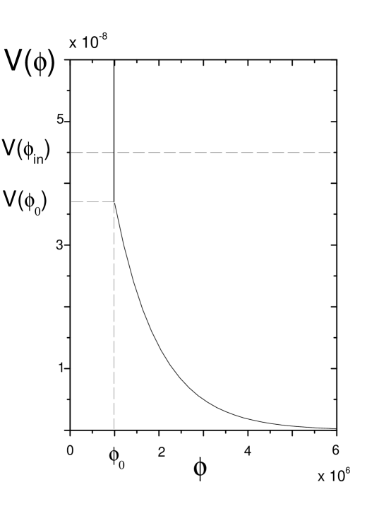
Figure 1: Tachyonic potential as a function of the tachyon field $\phi$. The values of the parameters were chosen as $A=10^{-7}\kappa^{-2}$ and $\lambda=10^{-5}\kappa^{-1/2}$, in units $\kappa=8\pi\,G=8\pi/M_{p}^{2}=1$.

The whole process is composed by different stages. The first stage corresponds to the creation of the closed universe “from nothing” in a state where the tachyon field takes the value $\phi_{in}\leq\phi_{0}$ at the point in which $\dot{a}=0$, $\dot{\phi}=0$, and where the potential energy is $V(\phi_{in})$ Balart:2007gs . If the effective potential for $\phi\ <\phi_{0}$ grows very sharply, then the tachyon field instantly falls down to the value $\phi_{0}$, with potential energy $V(\phi_{0})$, and the initial potential energy becomes converted to kinetic energy. Then, we find $\dot{\phi}^{2}_{0}=1-\left(\frac{V(\phi_{0})}{V(\phi_{in})}\right)^{2}$.

Following the discussion of the previous section we assume that the initial condition $\dot{\phi}^{2}<\frac{2}{3q}$ is satisfied. In terms of the potential this condition reads

$$\sqrt{\frac{3q-2}{3q}}<\frac{V(\phi_{0})}{V(\phi_{in})}<1,$$ (33)

which ensures that the patch cosmology enters to an inflationary regimen. As it was mentioned previously, in all other cases the universe either remains static or it collapses rapidly.

The other steps are described by Eqs.(13) and (14) in the interval $\phi\geq\phi_{0}$ with initial conditions $\dot{\phi}=\dot{\phi}_{0}$, $a=a_{0}$ and $\dot{a}=0$. In particular, the second part of the process corresponds to the motion of the tachyon field before the beginning of the inflation stage, and it is well described by the following approximated field equations of motion:

$$\frac{\ddot{\phi}}{1-\dot{\phi}^{2}}-3\,\frac{\dot{a}}{a}\,\dot{\phi}\,,$$ (34)

$$\ddot{a}=2\kappa_{1}\,a\,V(\phi)\,\beta(t),$$ (35)

where $\beta(t)$ satisfies the constraint $\beta(t)\ll 1$, as before.

The last statement corresponds to the stage of inflation where $\dot{\phi}$ is small enough and the scale factor $a(t)$ grows up exponentially. This period is well described by the following equations of motion Sami:2002fs ; Paul:2003jx :

$$3\,\frac{\dot{a}}{a}\,\dot{\phi}=-\frac{1}{V}\,\frac{dV}{d\phi}\,\,,$$ (36)

$$\ddot{a}=\kappa_{q}\,a\,V(\phi)^{q}\,.$$ (37)

Let us consider the second stage in a more detailed way. After the scheme of section III we can solve the equation for $a(t)$ by considering $\beta(t)\ll 1$. Then, at the beginning of the process, when $a\approx a_{0}$ and $\beta\approx\beta_{0}$, the increment of the tachyon field during the time $\Delta t$, which makes the value of $\beta$ twice as great as $\beta_{0}$, is $\Delta\phi\approx(3\,q\,\kappa_{q}\,V(\phi_{0})^{q})^{-1/2}$. This process continues until $\dot{\phi}$ is small enough so that the universe begins to expand in an exponential way, which characterizes the inflationary era. We assume that inflation begins when $\beta(t)$ approaches to $\beta_{f}$, where $\beta_{f}=\kappa_{q}\,V(\phi_{0})^{q-1}/(2\kappa_{1})$. Then, according to our previous result, the tachyon field gets the value

$$\phi_{inf}\sim\,\phi_{0}+\frac{1}{\ln 2}\;\!\left(\ln\beta_{f}-\ln\beta_{0}\right)\;\frac{1}{\sqrt{3\,q\,\kappa_{q}\,V(\phi_{0})^{q}}}.$$ (38)

During inflation, the scalar factor is given by

$$\frac{a}{a_{o}}=\exp\left(-3\kappa_{q}\,\int_{\phi_{o}}^{\phi}\,\frac{V^{q+1}}{dV/d\phi^{{}^{\prime}}}\,d\phi^{{}^{\prime}}\right),$$ (39)

and the corresponding $N$ e-folds results to be:

$$N=\frac{1}{2}\,\left[\left(\frac{V(\phi_{inf})}{V_{f}}\right)^{q}-1\right],$$ (40)

where $V_{f}=V(\phi_{f})=(q\,\lambda^{2}/(6\kappa_{q}))^{1/q}$ is the value of the tachyon potential at the end of inflation Paul:2003jx .

Then, by using Eqs.(38) and (40) we can relate the value of $\beta_{0}$ with the number of e-folds, $N$:

$$\beta_{0}=\left(\frac{\kappa_{q}\,V(\phi_{0})^{q-1}}{2\kappa_{1}}\right)\;\left[\frac{q\,\lambda^{2}\,(2N+1)}{6\kappa_{q}\,V(\phi_{0})^{q}}\right]^{\left(\frac{\ln 2}{q\,\lambda}\right)\sqrt{3q\kappa_{q}\,V(\phi_{0})}}.$$ (41)

Note that, in the case $q=1$, we recover the previous result obtained in Ref.Balart:2007gs .

Let us assume for definiteness that for $N=60$ one would have $\Omega=1.1$. Then one can show that for $N=59.5$ and the same value of the Hubble constant one would have $\Omega\approx 1.3$ Linde:2003hc ; Balart:2007gs . In order to have the value of $\Omega$ in the range $1\leq\Omega<1.1$ we require a fine tuning of the value of $V(\phi_{0})$.

Now, we are going to compute the value of the scalar field $\phi_{0}$. For this, we consider the mass of the tachyon to be $\lambda=10^{-5}\kappa^{-1/2}$ and the number of e-folds $N=60$. Then, for the case $q=1$ and if we assume $\phi_{0}\sim 10^{5}\kappa^{1/2}$, then in order to satisfy $\beta_{0}<V(\phi_{0})/M_{p}^{4}$ we have $\beta_{0}<2\times 10^{-10}$. Following Refs.Linde:2003hc and Balart:2007gs we see that the probability to begin with the value $\beta_{0}\ll\,2\times 10^{-10}$ is suppressed due to the small phase space corresponding to this value of $\beta_{0}$. Thus, it is most probable to have $\beta_{0}\sim 2\times 10^{-10}$, and in this case, if we set $\phi_{0}=1.1\times 10^{5}\kappa^{1/2}$, which satisfies the condition $\beta_{0}<V(\phi_{0})/M_{p}^{4}$, we obtain $N=60$ which correspond to $\Omega=1.1$. On the other hand, if we take $\phi_{0}=0.5\times 10^{5}\,\kappa^{1/2}$, we get N = 171 and the universe becomes flat. In the case $q=2$, following the same argument as before, we have $\beta_{0}\sim 10^{-12}$ then, for $N=60$ which correspond to $\Omega=1.1$, we set $\phi_{0}\simeq 3\times 10^{5}\kappa^{1/2}$. For $q=2/3$ we have $\beta_{0}\sim 10^{-11}$ and $\phi_{0}\sim 1.5\times 10^{5}\kappa^{1/2}$. We would like to note that the only way to obtain inflationary universe with $\Omega>1$ is to assume that the universe inflated only by about $e^{60}$ times. In order to explain this point we assume that for $N=60$ one would have $\Omega=1.1$ for all values of patch parameter $q$. Then, it is possible to show that for N = 59.5 one would have $\Omega=1.3$, whereas for $N=60.5$ one would have $\Omega=1.03$ corresponding to a marginally closed universe. Then, for $N>60$ (i.e $\phi_{0}<1.1\times 10^{5}\kappa^{1/2}$, which q=1, $\phi_{0}<3\times 10^{5}\kappa^{1/2}$ which $q=2$ and $\phi_{0}<1.5\times 10^{5}\kappa^{1/2}$ for $q=2/3$) the universe becomes flat. Thus in order to obtain $\Omega=1.1\pm 0.05$ one would need to have $N=60$ with accuracy of about 1 Linde:2003hc .

V Perturbations

The consequences of the dynamics of a closed inflationary universe, such as, slow roll parameters, density perturbations and tensor perturbations are quite complicate to be realized, since it involves several contributions. As it was shown in Refs. Linde:2003hc ; Balart:2007je ; delCampo:2004gh ; del Campo:2004ee ; del Campo:2004ee1 ; ramon , in a closed inflationary universe model this correction should be somewhat modified during the very first stages of the inflationary period, at $N={\cal O}(1)$. For instance, if we consider $N\geq 60$ in order to solve the cosmological ”puzzles”, we may get rid of the corrections and consider the standard flat-space expressions which gives correct results for $N>3$. In particular, the amplitude of scalar perturbations for a flat space, generated during tachyon inflation is defined in Ref. Hwang:2002fp

$$P_{\cal R}=\left(\frac{H^{2}}{2\pi\dot{\phi}}\right)^{2}\;\frac{1}{V}.$$ (42)

One interesting parameter to consider is the so-called spectral index $n_{s}$, which is related to $P^{1/2}_{\cal R}(k)$ Hwang:2002fp . For modes with a wavelength much larger than the horizon ($k\ll aH$), the spectral index $n_{s}$ is an exact power law, expressed by $P^{1/2}_{\cal R}(k)\propto k^{n_{s}-1}$, where $k$ is the comoving wave number. From WMAP five-year data it is obtained the values $P_{\cal R}\simeq 2.4\times\,10^{-9}$ and the spectral index $n_{s}\simeq 0.96$ ($\Lambda$CDM model) WMAP3 ; WMAP3a .

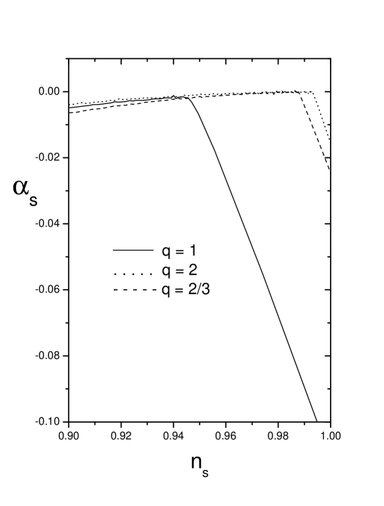
Figure 2: The plot shows the running of the scalar spectral index $\alpha_{s}$ as a function of the $n_{s}$. We have taken $\sigma=10^{-10}$, $\kappa_{2/3}=10^{-3}$ and we have used unit where $m_{p}=1$.

In tachyon inflationary models the scalar spectral index $n_{s}$ and the tensor spectral index $n_{T}$ are given by

$$n_{s}=1-2\,(2\epsilon_{1}-\epsilon_{2}+\epsilon_{3}),$$ (43)

and

$$n_{T}=-2(\epsilon_{1}-\epsilon_{3}),$$ (44)

in the slow-roll approximation Hwang:2002fp ; Hwang:2002fp1 ; Hwang:2002fp2 . Here, the slow-roll parameters are defined by:

$$\epsilon_{1}\simeq-\frac{\dot{H}}{H^{2}}\,,\;\;\epsilon_{2}\simeq-\frac{\ddot{\phi}}{H\,\dot{\phi}}\;,\;\epsilon_{3}\simeq\;-\left(\frac{\dot{\phi}}{2\,H\,V}\right)\,\frac{dV}{d\phi}.$$ (45)

One of the features of the five-year data set from WMAP is that it suggests a significant running in the scalar spectral index $dn_{s}/d\ln k=\alpha_{s}$ WMAP3 ; WMAP3a . From Eq.(43) we obtain that the running of the scalar spectral index for our model becomes

$$\alpha_{s}=\frac{dn_{s}}{d\ln k}\simeq\;\left(\frac{2V_{,\;\phi}}{3\kappa_{q}\,V^{q+1}}\right)\,[2\;\epsilon_{1\;,\;\phi}-\epsilon_{2\;,\;\phi}+\epsilon_{3\;,\;\phi}],$$ (46)

where we have used that $d\ln k=-dN$.

In models with only scalar fluctuations, the marginalized value for the derivative of the spectral index is approximated to $dn_{s}/d\ln k=\alpha_{s}\sim-0.03$ for WMAP five-year data only WMAP3 ; WMAP3a .

In Fig.2 we plot the running spectral index $\alpha_{s}$ versus the scalar index $n_{s}$ . In doing this, we have taken three different values of the patch parameter $q$, for the same initial condition. We note that for $n_{s}=0.97$, we obtain $\alpha_{s}\simeq-0.0482$, $\alpha_{s}\simeq-0.0003$ and $\alpha_{s}\simeq-0.0005$ for $q=1$, $q=2$, and $q=2/3$, respectively.

VI Conclusion and Final Remarks

In this paper we have studied a single tachyonic field in closed inflationary universe models in which the gravitational effects are described by patch cosmology. In this theory, the Friedmann equation has a complicated structure shown by Eq. (2) and in the limits of Gauss-Bonnet, high energy Randall Sundrum II model and 4D regime we obtain an effective Friedmann equation whose form is given by: $H^{2}\sim\rho^{q}$, where $q=2/3$, $q=2$ and $q=1$ for the GB, high energy brane world cosmology and 4D Einstein’s Theory of Relativity, respectively. We studied the patch cosmologies for two different models, corresponding to a constant potential and to a self-interacting tachyonic potential given by $V=V_{0}\exp(-\lambda\,\phi)$, ($\lambda>0$). In the first scenario, we have considered a potential with two regimes, one where the potential is constant and another one where the effective potential sharply rises to infinity. In the context of Einstein’s theory of GR, this model was studied by Linde Linde:2003hc with one standard scalar field. He showed that this model was not satisfactory because a constant potential implies that the universe collapses too soon or inflates forever. The tachyonic case was studied in Ref. Balart:2007gs in this model it was shown that it is less restrictive than the former. In our cases, we can fix the graceful exit problem because in patch cosmologies we have some extra ingredients related to the value of the patch parameter $q$ and the patch gravitational constant $\kappa_{q}$, that allows to reach the value $\dot{\phi}^{2}=2/3q$, which is needed to terminate inflation, see Eq.(21). The inclusion of corrections to the gravitational theory changes some of the characteristic of the perturbations. For instance, in patch cosmologies we found that the characteristic of the running spectral index $\alpha_{s}=0$ (standard theory pp1 ) changes to $\alpha_{s}\neq 0$ by virtue of equation (43). In particular for $n_{s}=0.97$, we obtain $\alpha_{s}\simeq-0.0482$, $\alpha_{s}\simeq-0.0003$ and $\alpha_{s}\simeq-0.0005$ for $q=1$, $q=2$, and $q=2/3$, respectively. These values are not far from the values given by WMAP five-year data WMAP3 ; WMAP3a .

Summarizing, we have been successful in describing a closed inflationary universe in a patch cosmology with a tachyon field theory.

- (1) C.L. Bennett et al.Astrophys. J. Suppl. 148, 1 (2003).
- (2) J. Dunkley et al. [WMAP Collaboration], Astrophys. J. Suppl. 180, 306 (2009).
- (3) G. Hinshaw et al. [WMAP Collaboration], Astrophys. J. Suppl. 180, 225 (2009).
- (4) P. de Bernardis et al Nature 404, 955 (2000).
- (5) J.E. Ruht et al, Astrophys.J. 599, 786 (2003)
- (6) A. Benoit et al, Astron.Astrophys 399, L25 (2003).
- (7) A. Guth Phys. Rev. D 23, 347 (1981).
- (8) J. P. Uzan, U. Kirchner and G. F. R. Ellis, Mon.Not.Roy.Astron.Soc.L 65, 344 (2003).
- (9) A. Linde, JCAP 0305, 002 (2003).
- (10) L. Randall and R. Sundrum, Phys. Rev. Lett. 83, 4690 (1999).
- (11) P. Binetruy, C. Deffayet and D. Langlois, Nucl. Phys. B565, 269 (2000).
- (12) P. Binetruy, C. Deffayet, U. Ellwanger, and D. Langlois, Phys. Lett. B477, 285 (2000).
- (13) R. Maartens, D. Wands, B. A. Bassett, and I. P. Heard, Phys. Rev. D 62, 041301 (2000).
- (14) A. R. Liddle and A. N. Taylor, Phys. Rev. D 65, 041301 (2002).
- (15) E. Ramirez and A. R. Liddle, Phys. Rev. D 69 083522 (2004).
- (16) S. Tsujikawa and A. R. Liddle, JCAP 0403, 001 (2004).
- (17) G. Calcagni, Phys. Rev. D 69, 103508 (2004).
- (18) Kyong Hee Kim, H. W. Lee, and Y. S. Myung, Phys. Rev. D 70, 027302 ( 2004).
- (19) A. Sen, JHEP 9808, 012 (1998); A. Sen, JHEP 9910, 008 (1999).
- (20) G. W. Gibbons, Phys. Lett. B 537, 1 (2002).
- (21) M. Fairbairn and M. H. G. Tytgat, Phys. Lett. B 546, 1 (2002).
- (22) M. Sami, P. Chingangbam and T. Qureshi, Phys. Rev. D 66, (2002) 043530.
- (23) D. Choudhury, D. Ghoshal, D. P. Jatkar and S. Panda, Phys. Lett. B 544, 231 (2002).
- (24) L. Kofman and A. Linde, JHEP 0207, 004 (2002)
- (25) X. z. Li, J. g. Hao and D. j. Liu, Chin. Phys. Lett. 19, 1584 (2002)
- (26) F. Leblond and A. W. Peet, JHEP 0304, 048 (2003).
- (27) S. Nojiri and S. D. Odintsov, Phys. Lett. B 571, 1 (2003).
- (28) S. Kachru, R. Kallosh, A. Linde, J. M. Maldacena, L. McAllister and S. P. Trivedi, JCAP 0310, 013 (2003).
- (29) Z. K. Guo and Y. Z. Zhang, JCAP 0408, 010 (2004)
- (30) D. J. Liu and X. Z. Li, Phys. Rev. D 70, 123504 (2004).
- (31) J. M. Aguirregabiria and R. Lazkoz,Phys. Rev. D 69, 123502 (2004).
- (32) J. M. Aguirregabiria and R. Lazkoz, Mod. Phys. Lett. A 19, 927 (2004).
- (33) X. H. Meng and P. Wang, Class. Quant. Grav. 21, 2527 (2004).
- (34) K. Hotta, Prog. Theor. Phys. 112, 653 (2004).
- (35) K. Hotta, JHEP 0603, 070 (2006).
- (36) L. Balart, S. del Campo, R. Herrera, P. Labrana and J. Saavedra, Phys. Lett. B 647, 313 (2007).
- (37) L. Balart, S. del Campo, R. Herrera and P. Labrana, Eur. Phys. J. C 51, 185 (2007).
- (38) C. Charmousis and J. F. Dufaux, Class. Quant. Grav. 19, 4671 (2002).
- (39) S. C. Davis, Phys. Rev. D 67, 024030 (2003).
- (40) E. Gravanis and S. Willison, Phys. Lett. B 562, 118 (2003).
- (41) J. E. Lidsey and N. J. Nunes, Phys. Rev. D 67, 103510 (2003).
- (42) S. Tsujikawa, M. Sami and R. Maartens, Phys. Rev. D 70, 063525 (2004).
- (43) J.E. Lidsey and N.J. Nunes, Phys. Rev. D 67, 103510 (2003).
- (44) K. i. Maeda and T. Torii, Phys. Rev. D 69, 024002 (2004).
- (45) J. F. Dufaux, J. E. Lidsey, R. Maartens and M. Sami, Phys. Rev. D 70, 083525 (2004).
- (46) G. Calcagni, JHEP 0509, 060 (2005).
- (47) M. Sami, P. Chingangbam and T. Qureshi, Phys. Rev. D 66, 043530 (2002).
- (48) B. C. Paul and M. Sami, Phys. Rev. D 70, 027301 (2004).
- (49) S. del Campo, R. Herrera and J. Saavedra, Phys. Rev. D 70, 023507 (2004).
- (50) S. del Campo, R. Herrera and J. Saavedra, Int. J. Mod. Phys. D 14, 861 (2005).
- (51) S. del Campo and R. Herrera, Class.Quant.Grav.22, 2687 (2005).
- (52) S. del Campo and R. Herrera, Phys.Rev.D 67, 063507 (2003).
- (53) J. C. Hwang and H. Noh, Phys. Rev. D 66, 084009 (2002).
- (54) M. R. Garousi, M. Sami and S. Tsujikawa, Phys. Rev. D 70, 043536 (2004).
- (55) S. Panda, M. Sami and S. Tsujikawa, Phys. Rev. D 73, 023515 (2006).
- (56) G. Ballesteros, J.A. Casas and J.R. Espinosa, JCAP 0603, 001 (2006).