Monte Carlo Study of an Inhomogeneous Blume-Capel Model

Abstract

Systems of particles in a confining potential exhibit a spatially dependent density which fundamentally alters the nature of phase transitions that occur. A specific instance of this situation, which is being extensively explored currently, concerns the properties of ultra-cold, optically trapped atoms. Of interest is how the superfluid-insulator transition is modified by the inhomogeneity, and, indeed, the extent to which a sharp transition survives at all. This paper explores a classical analog of these systems, the Blume-Capel model with a spatially varying single ion anisotropy and/or temperature gradient. We present results both for the nature of the critical properties and for the validity of the “local density approximation” which is often used to model the inhomogeneous case. We compare situations when the underlying uniform transition is first and second order.

Introduction

The realization of superfluid and Mott insulator transitions in optically trapped atoms greiner01 ; greiner02 ; stoferle04 has led to an examination of the nature of phase transitions in the presence of a spatially varying potential. For example, it was found that when a confining potential is added to the Bose-Hubbard Hamiltonian, the variation of density across the sample results in a coexistence of superfluid and Mott insulator regions batrouni02 ; batrouni08 . As a consequence, critical phenomena which occur in the uniform case, when the entire system collectively makes a transition from one phase to another, are smeared. The density no longer exhibits a singularity as a function of chemical potential, as occurs in the translationally invariant case fisher89 ; batrouni90 . Measures of “local quantum criticality” can be defined to help draw out residual signals of the global phase transition rigol03 .

These conclusions have been drawn from direct examination of the inhomogeneous model, but have also been inferred from studies of the translationally invariant model combined with the “local density approximation” (LDA) bergkvist04 . Specifically, the LDA assumes that the properties of the confined system at a particular spatial location are identical to those of the unconfined system with a uniform potential taking the same value as the local potential at that location. Various checks have been made, for example by comparing the LDA results using quantum monte carlo (QMC) of a collection of uniform systems, with QMC simulations of a lattice with a real trap bergkvist04 ; batrouni08 .

This LDA approximation is of course in direct analogy with that commonly used in density functional theory lundqvist83 , where the exact exchange-correlation potential present at a particular position ${\bf r}$, in a system where the electron density varies spatially, is replaced by the exchange correlation energy of the uniform electron gas at the same constant density as that present at ${\bf r}$. It is known that this approximation yields very good results in a number of contexts, especially when the electron-electron interactions are of weak to intermediate strength. On the other hand, when the coupling is stronger, and phenomena like magnetism and Mott transitions occur, the LDA is less accurate kotliar06 .

In this paper, we examine the nature of phase transitions in spatially inhomogeneous systems, and the validity of the LDA, within a more simple classical context. Previous work in this area includes studies of Ising transitions in systems with a temperature gradient where the nature of the interface between ferromagnetic regions adjacent to the “cold side” ($T<T_{c}$) of a sample and paramagnetic regions next to the “hot side” ($T>T_{c}$) has been explored Boissin91 ; Batrouni92 ; Platini07 ; Hansen92 .

Model and Calculational Approach

A classical model which can be constructed to have a spatially varying density similar to that in optically trapped atom systems is the Blume-Capel model Blume66 ; Capel66 with a site dependent single-ion anisotropy,

$$E=-J\sum_{\langle{\bf ij}\rangle}S_{\bf i}S_{\bf j}+\sum_{\bf i}\Delta_{\bf i}S_{\bf i}^{2}\,\,.$$ (1)

Here $S_{\bf i}$ is a discrete classical variable which can take on three values, $S_{\bf i}=0,\pm 1$. A coupling $J$ is present between near-neighbor spins which we choose to be positive (ferromagnetic). We consider a square lattice of linear size $L$. That is, ${\bf i}=(i_{x},i_{y})$ with $1\leq i_{x},i_{y}\leq L$. The value $S_{\bf i}=0$ can be thought of as corresponding to a vacancy, while $S_{\bf i}=\pm 1$ is an Ising spin, a collection of which can order ferromagnetically if the ratio of $J$ to temperature $T$ is sufficiently large. $\Delta$ is the single-ion anisotropy parameter, and controls the density of $S_{\bf i}=0$ spins.

The Blume-Capel model was originally introduced by Blume Blume66 and Capel Capel66 , separately, to study first-order magnetic transitions. It was later generalized to the Blume-Emery-Griffiths model (BEG) BEGriffiths , which incorporates an additional biquadratic interaction $K\sum_{\langle{\bf ij}\rangle}S_{\bf i}^{2}S_{\bf j}^{2}$. Since their initial fomulation, the Blume-Capel and BEG models have been extensively used to study the phase separation of He³-He⁴ mixtures BEGriffiths and various other systems that exhibit tricritical behavior, such as multicomponent fluids Lajzerowicz75 and semiconductor alloys Newman83 . Recent works have used the Blume-Capel model to study ferromagnetic thin films using an alternating single-ion anisotropy Zahraouy04 , and the dynamics of rough surfaces Brito07 .

Our computational method is standard Metropolis Monte Carlo. Each spin of the lattice is visited and a change from the current spin value to one of the two other possibilities is suggested. This change is accepted or rejected with the Metropolis prescription. To ensure equilibration, a large number of sweeps of all the spins in the lattice is performed prior to making measurements. Unless otherwise noted, the statistical errors in our results are smaller than the symbol size. The lattices studied in the manuscript are small enough that it is not necessary to emply more powerful cluster algorithms such as those developed by Swendsen and Wang swendsen87 .

For uniform systems, an accurate determination of the critical point can be obtained from computing the second moment of the magnetization landau00 ,

$$\langle\,M^{2}\,\rangle(T,L)=\frac{1}{L^{4}}\langle\,\,(\sum_{\bf i}S_{\bf i})^{2}\,\,\rangle\,\,.$$ (2)

Near the critical temperature, $T_{c}$, the following finite size scaling expression holds,

$$\langle M^{2}\rangle(T,L)=L^{-2\beta/\nu}f[L^{1/\nu}(T_{c}-T)]\,\,.$$ (3)

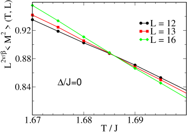
Here $\beta$ ($\nu$) are the critical exponents governing how the magnetization (correlation length) vanishes (diverges) as $T\rightarrow T_{c}$ in the thermodynamic limit. Eq. 3 implies that plots of $L^{2\beta/\nu}\,\langle M^{2}\rangle$ for different lattice sizes $L$ cross at $T=T_{c}$, providing a method to locate the critical temperature.

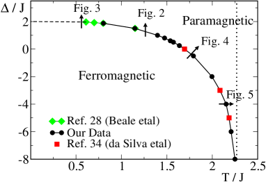
The physics of the Blume-Capel model with uniform $\Delta_{\bf i}=\Delta$ is well understood. When $\Delta\rightarrow-\infty$, vacancies ($S_{\bf i}=0$) are energetically very unfavorable. The system reduces to the Ising model and there is, on a square lattice, a second order magnetic phase transition at $T_{c}=2.269J$. We can also deduce the critical coupling at zero temperature. The energy of the fully polarized ferromagnetic state (all $S_{\bf i}=+1$) is $E_{\rm ferro}=(-2J+\Delta)L^{2}$. The energy of the empty state (all $S_{\bf i}=0$) is $E_{\rm vacuum}=0$. The ferromagnetic phase is favored up until $\Delta>2J$. Thus the phase diagram in the $(T/J,\Delta/J)$ plane consists of a ferromagnetic region at low $T/J$ and low $\Delta/J$ bounded by the lines $T/J=2.269$ and $\Delta/J=2$. As $\Delta$ increases from $\Delta=-\infty$ the extra entropy of vacancies reduces $T_{c}$ until the Ising limit boundary bends over to contact the $T=0$ critical point.

The phase boundary for uniform $J,\Delta$ has been obtained by a number of methods, including Monte Carlo simulations Wang87 ; Care93 ; Deserno97 , finite-size scaling PDBeale86 ; Plascak98 , renormalization group methods Berker76 ; Burkhardt76 , and series expansions Saul74 . From these studies it is knownPlascak98 that there is a tricritical point along the phase boundary at $(T/J,\Delta/J)=(0.609(4),1.965(5))$. At low temperatures in the vicinity of the $T=0$ critical point $(T/J,\Delta/J)=(0,2)$ the magnetization jumps discontinuously upon leaving the ferromagnetic phase. Beyond the tricritical point, the transition becomes continuous (second order). The phase boundary for this model is shown in Figure 1(top), where the values for $T_{c}$ were obtained through the analysis of Eqs. 2,3 using our code and from Ref. PDBeale86, and Silva02, . Figure 1(bottom) shows a representative finite size scaling crossing for $\Delta/J=0$. Table 1 provides the locations of $T_{c}$ for various values of $\Delta$.

Figure 1: (color online) Top: Phase diagram of the Blume Capel model at uniform $\Delta_{\bf i}=\Delta$. Second (first) order phase transitions are indicated by the solid (dashed) lines. The dotted line is the Ising limit. The four diamonds depict values from Ref. PDBeale86, . The squares are taken from Ref. Silva02, . The rest of boundary was obtained using our code and the finite size scaling analysis of Eq. 3. The arrows denote the trajectories used in the simulations of the inhomogeneous system, and correspond to Figs. 2,3,4,5 as indicated. See text. Bottom: A representative finite-size scaling analysis is shown. Here $\Delta=0$. The critical temperature $T_{c}$ is determined by the position of the universal crossing of the scaled second moment of magnetization for different linear lattice sizes.

$\hskip 14.45377pt\Delta/J$	$k_{B}T_{c}/J$	$k_{B}T_{c}/J$	$k_{B}T_{c}/J$
	(this work)	(Ref. PDBeale86, )	(Ref. Plascak98, )
-8	2.250(4)
-4	2.153(3)
-0.5	1.794(3)		1.794(7)
0	1.686(2)	1.695	1.681(5)
1	1.397(1)	1.398
1.87	0.802(2)	0.800

Table 1: Table of the critical temperatures for various values of $\Delta/J$ that were found using our code and finite-size scaling technique, in comparison with those from Refs. PDBeale86, and Plascak98, . The value at $\Delta/J=-8$, where vacancies are strongly suppressed, is close to the $T_{c}/J=2.269$ of the two dimensional Ising model, as expected.

Having reviewed and reproduced some of the features of the transitionally invariant Blume-Capel model, we now turn to the subject of this paper, the inhomogeneous case. We choose three models of spatial inhomogeneity. In the first two we introduce a linear variation of either the single-ion anisotropy or the temperature, keeping the other parameters fixed,

$$\Delta({\bf i}) = \Delta_{0}+\frac{\Delta_{1}-\Delta_{0}}{L_{x}}\,\,i_{x},\ \ \ \ T={\rm const}$$

$$T({\bf i}) = T_{0}+\frac{T_{1}-T_{0}}{L_{x}}\,\,i_{x},\ \ \ \ \Delta={\rm const}$$ (4)

These correspond to vertical ($\Delta$ varying) and horizontal ($T$ varying) cuts in the phase diagram. In the third case we allow both temperature and single ion anisotropy to change together,

$$\Delta({\bf i}) = \Delta_{0}+\frac{\Delta_{1}-\Delta_{0}}{L_{x}}\,\,i_{x},$$

$$T({\bf i}) = m\Big{(}\,\Delta_{1}+\frac{\Delta_{1}-\Delta_{0}}{L_{x}}\,\,i_{x}\,\Big{)}$$ (5)

where $m$ determines the slope of $T({\bf i})$. This more general inhomogeneity allows us to follow paths in the $(T,\Delta)$ plane which are perpendicular to the phase boundary in the intermediate coupling regime where the boundary curves around from its low $T$ and large negative $\Delta$ limits. Typically we will be interested in cases where $\Delta_{0},\Delta_{1},T_{0}$ and $T_{1}$ are chosen such that the lattice is ferromagnetic on the left side, $i_{x}=1$, with very few vacancies, and then becomes paramagnetic for $i_{x}=L_{x}$. For simplicity, we have chosen a gradient only in one spatial direction $x$, so the iso-contours of the single ion anisotropy are vertical lines. In $d=2$ ultracold trapped gases, the iso-contours are typically circles around the trap center. However, we do not expect the results of our study to depend on the shape of the boundary between phases, only on the existence of the boundary itselfwessel .

We have imposed periodic boundary conditions (pbc) in both the $x$ and $y$ directions. Besides reducing finite size effects, the use of pbc avoids having edge sites with a smaller number of neighbors than in the bulk, a situation which would make the connection with the LDA less simple. However, there is one slightly tricky issue with the pbc. The pbc links in the $y$ direction by construction connect sites with the same $\Delta_{\bf i}$. In the x-direction, the pbc’s link sites with vastly different single ion anisotropies: $\Delta_{0}$ and $\Delta_{1}$. To avoid this problem, the simulations were run on lattices with linear size $2L_{x}+1$ in the x-direction with $\Delta_{\bf i}$ symmetric across the center of the lattice. In effect, a second copy of the lattice is connected to the $x=1$ boundary of the first, and the values of $\Delta_{\bf i}$ increase linearly back up to $\Delta_{1}$ at which point the pbc connection is established. A final point about the geometry is that when we explore finite sizes effects we will fix $L_{y}=50$ and increase $L_{x}$ at constant $(\Delta_{1}-\Delta_{0})$. This is done because the $x$ direction is the one along which the gradient is established and so increasing $L_{x}$ allows us to explore the limit where the anisotropy gradient becomes weaker and weaker. Each of the cases will be used in regions where the respective gradient is approximately perpendicular to the phase boundary, as shown in figure 1(top). This ensures that the critical region will be localized to a small area of the lattice.

We present results for the “linear structure factor,” which we define as,

$${\bf\cal S}(i_{x}) = \langle\,\frac{1}{L_{y}^{2}}(\sum_{i_{y}}S_{(i_{x},i_{y})})^{2}\,\rangle$$ (6)

$$= \frac{1}{L_{y}}\sum_{l_{y}}\langle\,S_{(i_{x},1)}S_{(i_{x},1+l_{y})}\,\rangle\,\,.$$

${\bf\cal S}(i_{x})$ sums up the spin-spin correlations for all separations $l_{y}=1,2,\cdots L$ with a given $i_{x}$. The pairs of sites in ${\bf\cal S}(i_{x})$ therefore all have the same value of $\Delta_{\bf i}$. This is a convenient (indeed essential) choice in order to make meaningful comparisons with the LDA which employs lattices of constant $\Delta$. In this way, ${\bf\cal S}(i_{x})$ is the natural generalization of the mean square magnetization (Eq. 2) used in the translationally invariant case.

We will also compare the energy for an inhomogeneous lattice with that obtained by the LDA. Similar considerations apply here as with the linear structure factor; we would like to compare observables for sets of sites with the same value of $\Delta_{\bf i}$. However, the energy involves links (in the x-direction) which connect sites with different $\Delta_{\bf i}$. For this reason we will present results for the energy associated with bonds only in the $y$ direction,

$$E_{y}(i_{x}) =-\frac{J}{L_{y}}\sum_{i_{y}}S_{(i_{x},i_{y})}S_{(ix,i_{y}+1)}$$ (7)

$$+\frac{1}{L_{y}}\sum_{i_{y}}\Delta_{(i_{x},i_{y})}S_{(i_{x},i_{y})}^{2}\,\,.$$

Results

Figure 2: (color online) The full lines depict the linear structure factor ${\cal S}$ versus $\Delta({\bf i})$ at $T/J=1.25$ for several different gradients in the single-ion potential. For all full lines $\Delta_{0}/J=-8.00$ and $\Delta_{1}/J=4.00$, but as $L_{x}$ increases the gradient $\delta\Delta=(\Delta_{1}-\Delta_{0})/L_{x}$ softens. The LDA result is the dashed curve, and is quantitively correct except in the transition region. As expected, the accuracy of the LDA improves as the gradient of the inhomogeneity decreases.

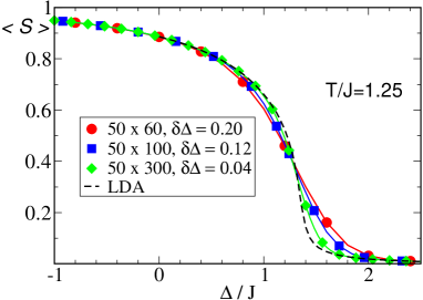
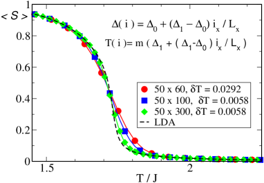
Figure 2 shows, for fixed $T/J=1.25$, the linear structure factor ${\cal S}$ as a function of $\Delta/J$. More precisely, ${\cal S}(i_{x})$ is computed at different values of $i_{x}$ for a system with a gradient $\delta\Delta=(\Delta_{1}-\Delta_{0})/L_{x}$ with $\Delta_{0}/J=-8.00$ and $\Delta_{1}/J=4.00$. The value of ${\cal S}(i_{x})$ is plotted against the corresponding value of $\Delta_{(i_{x},i_{y})}$ on the horizontal axis. Since the relation between $\Delta_{(i_{x},i_{y})}$ and $i_{x}$ is linear (Eq. 4), the horizontal axis can equivalently be viewed as labeling the spatial position as one sweeps across the inhomogeneous lattice. At the same time, the LDA values are obtained by simulating uniform systems at a range of $\Delta$ values corresponding to the vertical trajectory marked “Fig. 2” in the phase diagram of the uniform system, Fig. 1(top). This trajectory crosses the ferromagnetic to paramagnetic phase boundary at $\Delta=1.300(3)$ in a second order transition. We see that the LDA predicts the behavior of ${\cal S}$ in a qualitatively correct fashion over the entire range of $\Delta$, and is quantitively accurate except in the vicinity of the critical region where the lattice inhomogeneity blurs the transition. This is the same basic result as found for optically trapped atom systems batrouni02 ; batrouni08 . However, we are able in this simple classical model to compare more precisely the LDA with the inhomogeneous case. In particular, Fig. 2 shows the improved accuracy of the LDA as the gradient of the inhomogeneity becomes smaller, something which has not yet been done in the quantum case.

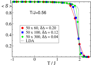
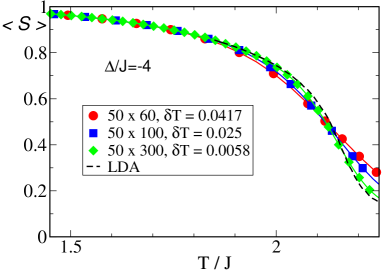
Fig. 3 shows a similar set of data but for $T/J=0.56$ which corresponds to the trajectory labeled “Fig. 3” in Fig. 1 and crosses the ferromagnetic-paramagnetic phase boundary in a first order transition at $\Delta/J=1.979(2)$. Again, the LDA is qualitatively correct. Comparing Figs. 2 and 3, it appears that the LDA has larger quantitative errors in the vicinity of the transition region in the first order case, but that these errors extend less far away from the transition region. This result seems reasonable: a smoothly varying potential does not exhibit the very abrupt discontinuity in the LDA results, but because the first order transition region is narrower, the region where LDA fails significantly is less wide. It is notable that curves of the linear structure factor for different values of the gradient cross at roughly a single point.

Figure 3: (color online) ${\cal S}$ versus $\Delta({\bf i})$ at $T/J=0.56$, a temperature below the tricritical point. Data are shown for several different values of the single-ion potential gradient (full curves). While the LDA predicts a first order phase transition (dashed curve), as is expected at this temperature, the phase transitions of the inhomogenous systems are less abrupt. As the variations in the single-ion potential decrease, or one moves far from the transition region, ${\cal S}$ converges to the results obtained by the LDA.

Our final two results for the linear structure factor are given in Figs. 4 and 5, and show cuts across the phase boundary in which both temperature and the single ion anisotropy are simultaneously evolving. The trajectories are labeled Figs. 4 and 5, in Fig. 1. The physics of our model does not depend independently on $T,\Delta_{\bf i},$ and $J$, but only on the ratios $\Delta_{\bf i}/T$ and $J/T$. In Fig. 2 only the first of these ratios is changing, while in Figs. 4 and 5 both ratios are evolving as we traverse the lattice. Since both of these cuts traverse the phase boundary in the second order region, the results for the LDA resemble those of Fig. 2. This emphasizes that the question of the accuracy of the LDA does not appear crucially to depend on which parameters in the energy (or the temperature) are varying.

Figure 4: (color online) The linear structure factor ${\cal S}$ versus $T(\Delta({\bf i}))$ for the inhomogenous case with both a spatially varying single-ion potential and temperature gradient. The choice $m=0.1458$ in Eq. 5 makes this trajectory cross perpendicular to the phase boundary.

Figure 5: (color online) The linear structure factor ${\cal S}$ versus $T({\bf i})$ at $\Delta/J=-4$ for several different values of temperature gradients.

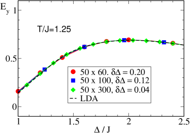
We now turn to a comparison of the energy of the inhomogeneous system with that of the LDA. Fig. 6 shows the same cut at constant $T/J=1.25$ as in Fig. 2. Remarkably, the energy is given very accurately by the LDA throughout the inhomogeneous lattice, even through the transition region where the linear structure factor differed markedly. This result may appear surprising in that the first piece of $E_{y}$ in Eq. 5 is the near neighbor spin correlation in the y-direction, which is also one of the ingredients of the linear structure factor ${\cal S}$. That the LDA value for $E_{y}$ is so accurate suggests that the failure of the LDA in the transition region is dominated by its mis-estimate of the long-range correlations, while the short range-ones are correctly identified. Indeed, this result might be expected since it is the long-range pieces of ${\cal S}$ whose behavior is crucial to the occurrence of a second order transition.

Figure 6: (color online) Comparison of the LDA prediction for the energy with the energy of an inhomogeneous system. Here we have fixed $T/J=1.25$ and are changing $\Delta_{\bf i}$ across the lattice. This is the trajectory labeled Fig. 2 in Fig. 1. The LDA energy is remarkably accurate even in the transition region.

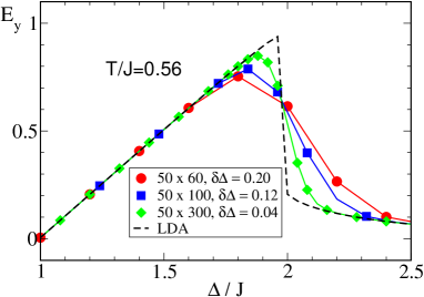
Finally, Fig. 7 shows the same cut at constant $T/J=0.56$ as in Fig. 3. Here, when the underlying homogeneous transition is first order, we see that even the energy is badly estimated by the LDA. The local energy has a universal crossing, corresponding to the transition value of $\Delta/J$, similar to that of the linear structure factor ${\cal S}$.

Figure 7: (color online) Comparison of the LDA prediction for the energy with the energy of an inhomogeneous system. Here we have fixed $T/J=0.56$ and are changing $\Delta_{\bf i}$ across the lattice. This is the trajectory labeled Fig. 3 in Fig. 1. Near the transition the LDA energy differs markedly from that of an inhomogeneous lattice.

Conclusions

The “Local Density Approximation” is a commonly employed method to understand the phase transitions of ultracold, optically trapped atoms which experience a spatially varying confining potential. In this paper we have explored the validity of the LDA in the simpler, classical, Blume-Capel model to which we have applied a gradient in the temperature and/or the single ion anisotropy.

Our basic conclusion is that the LDA performs well quantitatively in regions that are not close to where the state of the system is making a transition between the allowed phases, in our case ferromagnetic and paramagnetic. That is, the values of the local structure factor and energy predicted by the LDA match those of a direct simulation of the inhomogeneous system except in the transition zone. This is similar to the conclusions drawn in the optical lattice case batrouni02 . However, because our model is classical as opposed to quantum mechanical, we can explore the validity of the LDA in greater detail, including the systematic improvement in the accuracy of the LDA with inhomogeneous systems which have smaller gradients.

An especially interesting feature of the Blume-Capel model is the presence of a tricritical point on the phase boundary. This allows us to compare the validity of the LDA for first and second order transitions in the same model. Our conclusion is that a quantity like the linear structure factor which samples long range correlations is more badly estimated by the LDA in the transition region of a first order phase change, but that the width of the region over which the LDA is inaccurate is more narrow. Overall, the accuracy of the LDA in the two cases is not so dramatically different. On the other hand, the predictive accuracy of the LDA for the energy, which samples just short range correlations, is very different for the first and second order situations. In the second order case, the LDA energy is quantitativly correct even through the transition region, while in the first order case the energy is rather badly mis-estimated.

This work was supported by CNRS (France) PICS 18796 and ARO Award W911NF0710576 with funds from the DARPA OLE Program. We acknowledge useful input from T. Hollies.

References

- (1) M. Greiner, I. Bloch, O. Mandel, T.W. Hänsch, and T. Esslinger, Phys. Rev. Lett. 87, 160405 (2001).
- (2) M. Greiner, O. Mandel, T. Esslinger, T. W. Hänsch and I. Bloch, Nature 415, 39 (2002).
- (3) T. Stöferle, H. Moritz, C. Schori, M. Köhl, and T. Esslinger, Phys. Rev. Lett. 92, 130403 (2004).
- (4) G.G. Batrouni, V. Rousseau, R.T. Scalettar, M. Rigol, A. Muramatsu, P.J.H. Denteneer, and M. Troyer, Phys. Rev. Lett. 89, 117203 (2002).
- (5) G.G. Batrouni, H.R. Krishnamurthy, K. Mahmud, V.G. Rousseau, and R.T. Scalettar, Phys. Rev. A, to appear.
- (6) M.P.A. Fisher, P.B. Weichman, G. Grinstein, and D.S. Fisher, Phys. Rev. B40, 546 (1989).
- (7) G.G. Batrouni, R.T. Scalettar, and G.T. Zimanyi, Phys. Rev. Lett. 65, 1765 (1990).
- (8) M. Rigol, A. Muramatsu, G.G. Batrouni, and R.T. Scalettar, Phys. Rev. Lett. 91, 130403 (2003).
- (9) S. Bergkvist, P. Henelius, and A. Rosengren, Phys. Rev. A70, 053601 (2004).
- (10) Theory of the Inhomogeneous Electron Gas, edited by S. Lundqvist and S. H. March (Plenum, New York, 1983).
- (11) G. Kotliar, S. Y. Savrasov, K. Haule, V. S. Oudovenko, O. Parcollet, and C. A. Marianetti, Rev. Mod. Phys. 78, 865 (2006).
- (12) N. Boissin and H.J. Herrmann, J. Phys. A:Math Gen. 24, L43-L45 (1991).
- (13) G.G. Batrouni and A. Hansen, J. Phys. A:Math Gen. 25, L1059-L1064 (1992).
- (14) Gradients in the quantum Ising chain are explored in: T. Platini, D. Karevski, and L. Turban, J. Phys. A: Math. Theor. 40, 1467 (2007). The quantum Ising chain maps onto the 2d classical Ising model. This paper also includes a further review of the literature concerning inhomogeneities.
- (15) A. Hansen and D. Stauffer, Physica A189, 611 (1992).
- (16) M. Blume, Phys. Rev. 141, 517 (1966)
- (17) H.W. Capel, Physica 32, 966 (1966).
- (18) M. Blume, V.J. Emery, and R.B. Griffiths, Phys. Rev. A4, 1071 (1971).
- (19) J. Lajzerowicz and J. Sivardiere, Phys. Rev. A11, 2079 (1975).
- (20) K.E. Newman and J.D. Dow, Phys. Rev. B27, 7495 (1983).
- (21) H. Ez-Zahraouy and A. Kassou-Ou-Ali, Phys. Rev. B69, 064415 (2004).
- (22) A. Brito, J. A. Redinz, and J. A. Plascak, Phys. Rev. E75, 046106 (2007).
- (23) R.H. Swendsen and J-S. Wang, Phys. Rev. Lett. 58, 86 (1987).
- (24) “A Guide to Monte Carlo Simulations in Statistical Physics,” D.P. Landau and K. Binder, Cambridge University Press (2000).
- (25) Y. Wang, F. Lee, and J.D. Kimel, Phys. Rev. B36, 8945 (1987).
- (26) C. M. Care, J. Phys. A26, 1481 (1993).
- (27) M. Deserno, Phys. Rev. E56, 5204 (1997).
- (28) P.D. Beale, Phys. Rev. B33, 1717 (1986).
- (29) J.C. Xavier, F.C. Alcaraz, D.Pena Lara, and J.A. Plascak, Phys. Rev. B57, 11575 (1998).
- (30) A. N. Berker and M. Wortis, Phys. Rev. B14, 4946 (1976).
- (31) T. W. Burkhardt, Phys. Rev. B14, 1196 (1976)
- (32) D. M. Saul, M. Wortis, and D. Stauffer, Phys. Rev. B9, 4964 (1974).
- (33) S. Wessel, F. Alet, M. Troyer, and G. G. Batrouni, Phys. Rev. A70, 053615 (2004).
- (34) Roberto da Silva, Nelson A. Alves, and J.R. Drugowich de Felicio, Phys. Rev. E66, 026130 (2002).
- (35) I. B. Spielman, W. D. Phillips, and J. V. Porto, Phys. Rev. Lett. 100, 120402 (2008).