Deviations from Tri-bimaximal Mixing: Charged Lepton Corrections and Renormalization Group Running

Abstract

We analyze the effects of charged lepton corrections and renormalization group (RG) running on the low energy predictions of theories which accurately predict tri-bimaximal neutrino mixing at the high energy scale. In particular we focus on GUT inspired see-saw models with accurate tri-bimaximal neutrino mixing at the GUT scale, in which the charged lepton corrections are Cabibbo-like and give rise to sum rules valid at the GUT scale. We study numerically the RG corrections to a variety of such neutrino mixing sum rules in order to assess their accuracy and reliability when comparing them to future low energy neutrino oscillation experiments. Our results indicate that the RG corrections to neutrino mixing sum rules are typically small (less than one degree), at least in the examples studied with hierarchical neutrinos.

1 Introduction

Perhaps the greatest advance in particle physics over the past decade has been the discovery of neutrino mass and mixing involving two large mixing angles commonly known as the atmospheric angle $\theta_{23}$ and the solar angle $\theta_{12}$. The latest data from neutrino oscillation experiments is consistent with the so called tri-bimaximal (TB) mixing pattern [1],

$$U_{TB}=\left(\begin{array}[]{ccc}\sqrt{\frac{2}{3}}&\frac{1}{\sqrt{3}}&0\\ -\frac{1}{\sqrt{6}}&\frac{1}{\sqrt{3}}&\frac{1}{\sqrt{2}}\\ \frac{1}{\sqrt{6}}&-\frac{1}{\sqrt{3}}&\frac{1}{\sqrt{2}}\end{array}\right)P_{Maj},$$ (1.1)

where $P_{Maj}$ is the diagonal phase matrix involving the two observable Majorana phases, and there were many attempts to reproduce this as a theoretical prediction [2, 3, 4, 5, 6, 7, 8, 9, 10]. Since the forthcoming neutrino experiments will be sensitive to small deviations from TB mixing, it is important to study the theoretical uncertainty in such TB mixing predictions.

The question of how to achieve TM mixing has been the subject of intense theoretical speculation. In theoretical models one attempts to construct the neutrino and charged lepton mass matrices in some particular basis. There are two particular bases that have been used widely in the literature for this purpose, as follows. The first basis is the flavour basis in which the charged lepton mass matrix is diagonal, while the neutrino mass matrix takes a particular form such that is results in TB mixing. The second basis is a particular basis first introduced by Cabibbo and Wolfenstein in which both the neutrino and charged lepton mass matrices are non-diagonal, but in which the charged lepton mass matrix is diagonalised by a “democratic unitary matrix” involving elements of equal magnitude but differing by a phase $\omega=2\pi/3$. Such a Cabibbo-Wolfenstein basis is particularly well suited to models of TB mixing based on the discrete group $A_{4}$ [11]. However in other classes of models, one attempts to work in the flavour basis and to derive TB mixing purely from the neutrino sector with the charged lepton matrix being diagonal, for example using constrained sequential dominance (CSD) [2].

However, when attempting to derive TB mixing in the flavour basis in realistic models arising from Grand Unified Theories (GUTs), it is observed that, although TB mixing may be accurately achieved from neutrino mixing, in practice the flavour basis is never accurately achieved, i.e. the charged lepton mass matrix is never accurately diagonal. Instead, in such GUT models, the charged lepton mass matrix often resembles the down quark mass matrix, and involves an additional Cabibbo-like rotation in order to diagonalize it. In such models, then, TB mixing arises in the neutrino sector, but with charged lepton correction giving deviations [12]. It turns out that such Cabibbo-like charged lepton corrections lead to well defined corrections to TB mixing which can be cast in the form of sum rules expressed in terms of the measurable PMNS parameters. One example is the neutrino mixing sum rule $\theta_{12}-\theta_{13}\cos(\delta)\approx\theta_{12}^{\nu}$[2, 13, 14], where $\delta$ is the observable Dirac CP phase in the standard parameterisation. Since such sum rules may be tested in future high precision long baseline neutrino experiments, it is of interest to know with what precision they are expected to hold theoretically.

Such sum rules as discussed above are strictly only expected to apply at some high energy scale, whereas the neutrino experiments are performed at low energy scales. In order to compare the predictions of such sum rules to experiment one must therefore perform a renormalisation group (RG) running from the high energy (e.g. the Grand Unified Theory (GUT)) scale where the theory is defined to the electroweak scale $M_{Z}$. RG corrections arise mainly from the large tau lepton and third family neutrino Yukawa couplings, and this leads to large wavefunction corrections in the framework of supersymmetric models. The running of neutrino masses and lepton mixing angles is very important and has been studied extensively in the literature [15]. In [16, 17] a mathematica package REAP (http://www.ph.tum.de/ rge/) which solves RGEs and provides numerical values for the neutrino mass matrix and mixing angles was developed.

In this paper we provide a first numerical study of the deviations from TB mixing due to the effects of both charged lepton corrections and RG running. We focus on GUT inspired models in which the charged lepton corrections are Cabibbo-like and in this case they may be cast in terms of sum rules valid at the GUT scale. In practice, then, we are interested in the RG corrections to these sum rules which may subsequently be reliably compared to experiment at low energies. We shall study a variety of neutrino mixing sum rules (arising from the deviations from exact tri-bimaximal neutrino mixing due to Cabibbo-like charged lepton corrections) and comment on their accuracy and reliability when comparing them to future low energy neutrino oscillation experiments. Most of the specific numerical results are inspired by a particular class of GUT-flavour models, namely the models in [2, 6], which are precisely the type of models in which the sum rules emerge in the first place. In the cases studied we find rather small corrections. For example the sum rule $\theta_{12}-\theta_{13}\cos(\delta)\approx 35.3^{o}$ becomes renormalized by about $0.4^{o}$ for large $\tan\beta=50$. Although most of the numerical results are based on a particular GUT motivated model, we also analyze a completely different type of model and find qualitatively similar results. This suggests that our results will apply to more general models based on the Minimal Supersymmetric Standard Model, extended to include the see-saw mechanism, with hierarchical neutrino masses.

We emphasize that in this paper we only consider deviations from TB lepton mixing due to the combination of charged lepton corrections and RG running, and that in general there will be other sources of deviations that we do not consider. For example, exact CSD [2] itself will lead to some deviations since it does not predict precisely TB neutrino mixing due to corrections of order $m_{2}/m_{3}$ [18]. Another example of deviations to TB mixing are the canonical normalization effects discussed in [19]. Clearly such additional corrections are quite model dependent and a phenomenological study of corrections to the TB mixing in the neutrino sector, in the flavour basis, has been made in [20]. In this paper we shall simply assume precise TB neutrino mixing at the GUT scale, and investigate the deviations due to charged lepton corrections and RG running only, ignoring other possible model dependent corrections. The RG corrections to TB mixing (but not charged lepton corrections or the resulting sum rules) were also considered in [21].

The layout of the remainder of the paper is as follows. In section 2 we give our conventions, including the TB deviation parameters that we will use. In section 3 we discuss the see-saw mechanism and show how TB neutrino mixing can be achieved. In section 4 we show how Cabibbo-like charged lepton corrections leads to neutrino mixing sum rules. We also present a numerical model of TB neutrino mixing adapted from a well motivated example of light sequential dominance used in the GUT flavour models of [2, 6] that we shall use in most of the remainder of the paper. We also show how sensitive these results are to non-Cabibbo like charged lepton corrections. In section 5 we numerically study the RG corrections to the various neutrino mixing sum rules which embody the charged lepton corrections to TB neutrino mixing. In section 6 we explore a second type of numerical model adapted from heavy sequential dominance [18] and show that the results are qualitatively similar to the case of the first numerical model. Section 7 concludes the paper.

2 Conventions

2.1 The PMNS matrix in the standard parametrization

The mixing matrix in the lepton sector, the PMNS matrix $U_{PMNS}$, is defined as the matrix appearing in the electroweak coupling to the $W$ bosons expressed in terms of lepton mass eigenstates. The Lagrangian is given in terms of mass matrices of charged leptons $M_{e}$ and neutrinos $m_{\nu}$ as,

$$\mathcal{L}=-\bar{e}_{L}M_{e}e_{R}-\frac{1}{2}\bar{\nu}_{L}m_{LL}\nu_{L}^{c}+H.c,$$ (2.1)

The change in basis from flavour to eigenbasis is performed by,

$$V_{e_{L}}M_{e}V_{e_{R}}^{\dagger}=diag(m_{e},m_{\mu},m_{\tau}),\hskip 8.53581ptV_{\nu_{L}}m_{LL}V_{\nu_{L}}^{T}=diag(m_{1},m_{2},m_{3}),$$ (2.2)

The PMNS matrix is then given by,

$$U_{PMNS}=V_{e_{L}}V_{\nu_{L}}^{\dagger}.$$ (2.3)

In the standard PDG parametrization, the PMNS matrix can be written as,

$$U_{PMNS}=\left(\begin{array}[]{ccc}c_{12}c_{13}&s_{12}c_{13}&s_{13}e^{-i\delta}\\ -c_{23}s_{12}-s_{13}s_{23}c_{12}e^{i\delta}&c_{23}c_{12}-s_{13}s_{23}s_{12}e^{i\delta}&s_{23}c_{13}\\ s_{23}s_{12}-s_{13}c_{23}c_{12}e^{i\delta}&-s_{23}c_{12}-s_{13}c_{23}s_{12}e^{i\delta}&c_{23}c_{13}\end{array}\right)P_{Maj},$$ (2.4)

where $\delta$ is the Dirac CP violating phase, and $P_{Maj}=diag(e^{i\frac{\alpha_{1}}{2}},e^{i\frac{\alpha_{2}}{2}},0)$ contains the Majorana phases $\alpha_{1}$, $\alpha_{2}$. The latest experimental values and errors for the three neutrino oscillation parameters are summarised inTable.1 [22, 23, 24].

Parameter	Best fit ($\,{}^{\circ}$)	2 $\sigma$ ($\,{}^{\circ}$)	3 $\sigma$ ($\,{}^{\circ}$)
$\theta_{12}$	34.44	31.94- 37.46	30.65- 39.23
$\theta_{23}$	45	38.05 - 52.53	35.66 - 54.93
$\theta_{13}$	4.79	$\leq$ 10.46	$\leq$ 12.92

Table 1: Best fit values, 2 $\sigma$ and 3 $\sigma$ intervals for the three- flavour neutrino oscillation parameters from global data including accelerator (K2K and MINOS) and solar, atmospheric, reactor (Kam LAND and CHOOZ) experiments [22].

2.2 A parametrization in terms of deviations

Another parametrisation of the lepton mixing matrix can be achieved by taking an expansion about the tri-bimaximal matrix. Three small parameters $r$, $s$ and $a$ are introduced to describe the deviations of the reactor, solar and atmospheric angles from their tri-bimaximal values [25],

$$s_{13}=\frac{r}{\sqrt{2}},\hskip 11.38109pts_{12}=\frac{1}{\sqrt{3}}(1+s),\hskip 11.38109pts_{23}=\frac{1}{\sqrt{2}}(1+a).$$ (2.5)

Global fits of the conventional mixing angles [24] can be translated into the ranges,

$$0<r<0.22,\hskip 11.38109pt-0.11<s<0.04,\hskip 11.38109pt-0.12<a<0.13.$$ (2.6)

Considering an expansion of the lepton mixing matrix in powers of $r$, $s$, $a$ about the tri-bimaximal form. One gets the following form for the mixing matrix to first order in $r$, $s$, $a$ [25],

$$U_{MNS}\approx\left(\begin{array}[]{ccc}\sqrt{\frac{2}{3}}(1-\frac{1}{2}s)&\frac{1}{\sqrt{3}}(1+s)&\frac{1}{\sqrt{2}}re^{-i\delta}\\ -\frac{1}{\sqrt{6}}(1+s-a+re^{i\delta})&\frac{1}{\sqrt{3}}(1-\frac{1}{2}s-a-\frac{1}{2}re^{i\delta})&\frac{1}{\sqrt{2}}(1+a)\\ \frac{1}{\sqrt{6}}(1+s+a-re^{i\delta})&-\frac{1}{\sqrt{3}}(1-\frac{1}{2}s+a+\frac{1}{2}re^{i\delta})&\frac{1}{\sqrt{2}}(1-a)\end{array}\right)P_{Maj}.$$ (2.7)

2.3 Third row deviation parameters

For later convenience, we also define the following parameters which express the deviation of the magnitude of the third row mixing matrix elements from their tri-bimaximal values:

$$|(U_{PMNS})_{31}| \equiv \frac{1}{\sqrt{6}}(1+\xi_{1})$$

$$|(U_{PMNS})_{32}| \equiv \frac{1}{\sqrt{3}}(1+\xi_{2})$$

$$|(U_{PMNS})_{33}| \equiv \frac{1}{\sqrt{2}}(1+\xi_{3})$$ (2.8)

Hence from Eq.2.4,

$$\begin{array}[]{ccc}\xi_{1}&=&\sqrt{6}~{}|s_{23}s_{12}-s_{13}c_{23}c_{12}e^{i\delta}|-1,\\ \xi_{2}&=&\sqrt{3}~{}|-s_{23}c_{12}-s_{13}c_{23}s_{12}e^{i\delta}|-1,\\ \xi_{3}&=&\sqrt{2}~{}|c_{23}c_{13}|-1.\end{array}$$ (2.9)

We can also express the $\xi_{i}$ parameters in terms of the deviation parameters $r$, $s$, $a$ from Eq.2.7as follows,

$$\begin{array}[]{ccc}\xi_{1}&\approx&|1+s+a-re^{i\delta}|-1,\\ \xi_{2}&\approx&|1-\frac{1}{2}s+a+\frac{1}{2}re^{i\delta}|-1,\\ \xi_{3}&\approx&|1-a|-1.\end{array}$$ (2.10)

3 The See-Saw Mechanism and TB Neutrino Mixing

3.1 The see-saw mechanism

The see-saw mechanism provides an excellent explanation for the smallness of neutrino masses. Before discussing its simplest form, we first start by summarising the possible types of neutrino mass.

One type is Majorana masses of the form $m_{LL}\bar{\nu_{L}}\nu_{L}^{c}$ where $\nu_{L}$ is a left-handed neutrino field and $\nu_{L}^{c}$ is the CP conjugate of a left- handed neutrino field, in other words a right handed antineutrino field [26]. Introducing right-handed neutrino fields, other neutrino mass terms are possible. There are additional Majorana masses of the form $M_{RR}\bar{\nu_{R}}\nu_{R}^{c}$ and Dirac masses of the form $m_{LR}\bar{\nu_{L}}\nu_{R}$ where $\nu_{R}$ is a right-handed neutrino field and $\nu_{R}^{c}$ is its CP conjugate.

The Majorana masses of the form $m_{LL}^{\nu}$are strictly forbidden in the standard model, assuming only the higgs doublets are present. The reason for this is that heavy left-handed neutrinos would disturb the theory of weak interactions with W, Z bosons. For the simplest version of the see-saw mechanism, one can assume that the left-handed Majorana masses are zero at first, but are effectively generated after introducing the right handed neutrinos [27].

The right-handed neutrino does not take part in weak interactions with the W, Z bosons, and so its mass $M_{RR}$ can be arbitrarily large. With these types of neutrino mass, the see-saw mass matrix is given as,

$$\left(\bar{\nu_{L}}\bar{\nu_{R}^{c}}\right)\left(\begin{array}[]{cc}0&m_{LR}\\ m_{LR}^{T}&M_{RR}\end{array}\right)\left(\begin{array}[]{cc}\nu_{L}^{c}\\ \nu_{R}\end{array}\right)$$ (3.1)

In the approximation that $M_{RR}\gg m_{LR}$ ( $M_{RR}$ may be orders of magnitude larger than the electroweak scale), the matrix in Eq.3.1 can be diagonalised to give the effective left-handed Majorana masses,

$$m_{LL}=m_{LR}M_{RR}^{-1}m_{LR}^{T}$$ (3.2)

These masses are naturally suppressed by the heavy scale $M_{RR}$. Taking $m_{LR}=M_{W}=80GeV$ and $M_{RR}=M_{GUT}=10^{16}GeV$, we find $m_{LL}\sim 10^{-3}eV$ which is good for solar neutrinos. A right-handed neutrino with a mass below the GUT scale would be required for atmospheric neutrinos.

The fundamental parameters which must be inputted into the see-saw mechanism are the Dirac mass matrix $m_{LR}$ and the heavy right-handed neutrino Majorana mass matrix $M_{RR}$. The output is the effective left-handed Majorana mass matrix $m_{LL}$ as given by the see-saw formula in Eq.3.2 [28].

The see-saw mechanism discussed so far is the simplest version and it is sometimes called type I see-saw mechanism. In Pati-Salam models or grand unified theories based on $SO(10)$, type I is generalised to type II see-saw, where an additional term for the light neutrinos is present [29].

3.2 Approximate TB neutrino mixing from CSD

Sequential dominance (SD) is an elegant way of accounting for a neutrino mass hierarchy with large atmospheric and solar mixing angles [30, 31]. Here we review how tri-bimaximal neutrino mixing can result from constrained sequential dominance (CSD) [2]. In SD, the atmospheric and solar neutrino mixing angles are obtained in terms of ratios of Yukawa couplings involving the dominant and subdominant right-handed neutrinos, respectively. To understand how tri- bimaximal neutrino mixing could emerge from SD, we begin by writing the right- handed neutrino Majorana mass matrix $M_{RR}$ in a diagonal basis as,

$$M_{RR}\approx\left(\begin{array}[]{ccc}Y&0&0\\ 0&X&0\\ 0&0&X^{\prime}\end{array}\right).$$ (3.3)

Without loss of generality write the neutrino (Dirac) Yukawa matrix $Y_{LR}^{\nu}$ in terms of the complex Yukawa couplings a,b,c,d,e,f,a’,b’,c’ as

$$Y_{LR}^{\nu}=\left(\begin{array}[]{ccc}d&a&a^{\prime}\\ e&b&b^{\prime}\\ f&c&c^{\prime}\end{array}\right).$$ (3.4)

For simplicity we assume that $d=0$. SD then corresponds to the right-handed neutrino of mass $Y$ being the dominant term while the right- handed neutrino of mass $X$ giving the leading sub-dominant contribution to the see-saw mechanism.

$$\frac{|e^{2}|,|f^{2}|,|ef|}{Y}\gg\frac{|xy|}{X}\gg\frac{x^{\prime}y^{\prime}}{X^{\prime}}$$ (3.5)

where $x,y\in a,b,c$ and $x^{\prime},y^{\prime}\in a^{\prime},b^{\prime}c^{\prime}$, and all Yukawa couplings are assumed to be complex. Light sequential dominance corresponds to

$$Y<X<X^{\prime}.$$ (3.6)

Tri-bimaximal neutrino mixing, in which $\tan\theta_{23}^{\nu}=1$, $\tan\theta_{12}^{\nu}=1/\sqrt{2}$ and $\theta_{13}^{\nu}=0$ corresponds to the choice,

$$|a| = |b|=|c|,$$ (3.7)

$$|d| = 0,$$ (3.8)

$$|e| = |f|$$ (3.9)

$$e^{*}b+f^{*}c = 0.$$ (3.10)

This corresponds to constrained sequential dominance (CSD)[2]. Note that the analytic results for SD and CSD are accurate to leading order in $m_{2}/m_{3}$ [18], so these conditions will not give rise precisely to TB neutrino mixing, and so in the numerical studies we shall need to perturb the CSD relations in order to achieve accurate TB neutrino mixing at the GUT scale, as discussed later.

4 Charged lepton corrections

4.1 Cabibbo-like corrections

4.1.1 Sum rules

In this paper we shall consider the case that TB mixing (Eq.1.1) applies quite accurately only to the neutrino mixing in some basis where the charged lepton mass matrix is not exactly diagonal [32]. This is a situation often encountered in realistic models [2]. Furthermore in GUT models it is often the case that, in the basis where the neutrino mixing is of the TB form, the charged lepton mixing matrix has a Cabibbo-like structure rather similar to the quark mixing and is dominated by a 1-2 mixing $\theta_{12}^{E}$ [33],

$$V_{e_{L}}=\left(\begin{array}[]{ccc}c_{\theta_{12}^{E}}&-s_{\theta_{12}^{E}}e^{-i\lambda_{12}^{E}}&0\\ s_{\theta_{12}^{E}}e^{i\lambda_{12}^{E}}&c_{\theta_{12}^{E}}&0\\ 0&0&1\end{array}\right),$$ (4.1)

where $c_{\theta_{12}^{E}}\equiv\cos\theta_{12}^{E}$, $s_{\theta_{12}^{E}}\equiv\sin\theta_{12}^{E}$, and $\lambda_{12}^{E}$ is a phase required for the diagonalisation of the charged lepton mass matrix [2]. The physical PMNS oscillation phase $\delta$ turns out to be related to $\lambda_{12}^{E}$ by [33],

$$\delta=\lambda_{12}^{E}+\pi.$$ (4.2)

In this paper we assume that the neutrino mixing is accurately of the TB form,

$$V_{\nu_{L}}^{\dagger}=\left(\begin{array}[]{ccc}\sqrt{\frac{2}{3}}&\frac{1}{\sqrt{3}}&0\\ -\frac{1}{\sqrt{6}}&\frac{1}{\sqrt{3}}&\frac{1}{\sqrt{2}}\\ \frac{1}{\sqrt{6}}&-\frac{1}{\sqrt{3}}&\frac{1}{\sqrt{2}}\end{array}\right)P_{Maj}.$$ (4.3)

The physical mixing matrix is given by Eq.2.3 using Eq.4.3 and Eq.4.1. The standard PDG form of the PMNS mixing matrix in Eq.2.4 requires real elements $(U_{PMNS})_{11}$ and $(U_{PMNS})_{12}$ and this may be achieved by use of the phases in $P_{Maj}=diag(e^{i\frac{\alpha_{1}}{2}},e^{i\frac{\alpha_{2}}{2}},0)$.

It follows that $(U_{PMNS})_{31}$, $(U_{PMNS})_{32}$ and $(U_{PMNS})_{33}$ are unaffected by the Cabibbo-like charged lepton corrections and are hence given by:

$$|(U_{PMNS})_{31}|=|(V_{\nu_{L}}^{\dagger})_{31}|=\frac{1}{\sqrt{6}},$$ (4.4)

$$|(U_{PMNS})_{32}|=|(V_{\nu_{L}}^{\dagger})_{32}|=\frac{1}{\sqrt{3}},$$ (4.5)

$$|(U_{PMNS})_{33}|=|(V_{\nu_{L}}^{\dagger})_{33}|=\frac{1}{\sqrt{2}}.$$ (4.6)

The relations in Eqs.4.4, 4.5, 4.6 may be expressed in terms of the third family matrix element deviation parameters defined in Eq.2.3 as simply:

$$\xi_{i}=0.$$ (4.7)

Since these relations are all on the same footing, it is sufficient to discuss one of them only and in the following we choose to focus on Eq. 4.4. From Eq.2.4, Eq. 4.4 may be expanded in terms of the standard mixing angles and phase leading to the so called mixing sum rules as follows:

$$\Gamma_{1}\equiv\arcsin\left(\sqrt{2}~{}|s_{23}s_{12}-s_{13}c_{23}c_{12}e^{i\delta}|\right)=35.26^{o},$$ (4.8)

where we have assumed $s_{23}^{\nu}\equiv\sin\theta_{23}^{\nu}=\frac{1}{\sqrt{2}}$. This sum rule can be simplified further to leading order in $s_{13}$,

$$\Gamma_{2}\equiv\arcsin\left(\sqrt{2}~{}(s_{23}s_{12}-s_{13}c_{23}c_{12}\cos{\delta})\right)\approx 35.26^{o}.$$ (4.9)

From Eq.4.6 $s_{23}=c_{23}=1/\sqrt{2}$, hence to leading order,

$$\Gamma_{3}\equiv\theta_{12}-\theta_{13}\cos(\delta)\approx 35.26^{o}.$$ (4.10)

The last form of the sum rule was first presented in [2], while all the forms can be found in [14]. We shall later study all three forms of the sum rules $\Gamma_{i}$, together with some related sum rules which we now discuss.

Using the parametrization in Eq.2.5, the sum rule in Eq.4.10 can be expressed in terms of the deviation parameters $s$, $r$ and the Dirac CP phase ($\delta$)[25],

$$\sigma_{1}=r\cos\delta-s=0.$$ (4.11)

To deal with issues of canonical normalisation corrections, the following sum rule has been proposed [19],

$$\sigma_{2}=r\cos\delta+\frac{2}{3}a-s=0.$$ (4.12)

This sum rule was claimed to be stable under leading logarithmic third family RG corrections, although, as emphasized in [19], it does not include the effect of the running of $\theta_{13}$ or $r$, whose inclusion introduces a Majorana phase dependence. Such effects will be studied numerically later.

4.1.2 A GUT-Flavour Inspired Numerical Example

In order to study the RG corrections and reliability of the various sum rules numerically it is necessary to define the GUT scale matrices rather specifically. In most of this paper we shall consider a numerical example inspired by the GUT-flavour models of [2, 6], although in Section 6 another numerical model will be considered leading to qualitatively similar results. Therefore in most of the remainder of this paper we shall take the right-handed neutrino Majorana mass matrix $M_{RR}$ to be the diagonal matrix:

$$M_{RR}=\left(\begin{array}[]{ccc}5.1\times 10^{-9}&0&0\\ 0&7.05\times 10^{-9}&0\\ 0&0&1\end{array}\right)M_{3},$$

where $M_{3}=10^{16}GeV$. This is an example with light sequential dominance where the lightest right handed neutrino is dominant [18]. Ignoring RGE corrections to begin with, we find that precise tri-bimaximal neutrino mixing ($\theta^{\nu}_{12}=35.26\,^{\circ}$, $\theta^{\nu}_{23}=45.00\,^{\circ}$, $\theta^{\nu}_{13}=0.00\,^{\circ}$) can be achieved with the Yukawa matrix:

$$Y_{LR}^{\nu}=\left(\begin{array}[]{ccc}0&1.061667b&0.001\\ e&b&0\\ -0.9799e&b&c_{3}\end{array}\right)$$ (4.13)

where $b=8.125\times 10^{-5}$, $e=2.125\times 10^{-4}$ and $c_{3}=0.5809$. These parameters also lead to the following values for the neutrino masses: $m_{1}=1.75\times 10^{-4}eV$, $m_{2}=8.67\times 10^{-3}eV$, $m_{3}=4.95\times 10^{-2}eV$, $\Delta m^{2}_{atm}=2.37\times 10^{-3}eV^{2}$ and $\Delta m^{2}_{sol}=7.52\times 10^{-5}eV^{2}$.

The low energy pole masses of the quarks are given as follows: $m_{u}=1.22~{}MeV$, $m_{d}=2.77~{}MeV$, $m_{s}=53~{}MeV$, $m_{c}=0.595~{}GeV$, $m_{b}=2.75~{}GeV$ and $m_{t}=163.6~{}GeV$. In order to satisfy these values at low energy scale, REAP was used to perform the running of these masses from the $M_{Z}$ scale to the GUT scale and the resulting quark Yukawa matrices $Y_{u}$ and $Y_{d}$ at the GUT scale were taken as initial conditions for the running of the neutrino mixing parameters and sum rules from the GUT scale to $M_{Z}$ scale.

The above parameter choice approximately satisfies the CSD conditions in Eq.3.7. However small corrections are used in order to achieve TBM neutrino mixing angles to 2 decimal places. If the CSD conditions were imposed exactly we would find instead $\theta_{12}=33.97\,^{\circ}$, $\theta_{23}=44.38\,^{\circ}$, $\theta_{13}=0.059\,^{\circ}$ and $\delta=0\,^{\circ}$ which are close to, but not accurately equal to, the TBM values. This is to be expected since the SD relations are only accurate to leading order in $m_{2}/m_{3}$ [18]. Since in this paper we are interested in studying the deviations from exact TB neutrino mixing due to charged lepton corrections and RG running we shall assume the matrices in Eq.4.13 rather than the CSD conditions as the starting point for our analysis.

In order to study the effect of Cabibbo-like charged lepton corrections on the physical mixing angles where the neutrino mixing is precisely tri-bimaximal, we shall use the REAP package previously discussed. In order to use the REAP package it is convenient to work in the basis where the charged lepton Yukawa matrix is diagonal. Thus, assuming charged lepton corrections of the form of Eq.4.1, the neutrino Yukawa matrix in the non-diagonal charged lepton basis must be transformed to the diagonal charged lepton basis according to:

$$Y_{\nu}\rightarrow Y^{\prime}_{\nu}=V_{e_{L}}Y_{\nu}.$$ (4.14)

Hence the original neutrino Yukawa matrix in Eq.4.13 must be rotated to the diagonal charged lepton basis according to Eq.4.14.

Including the Cabibbo-like charged lepton corrections, physical tri-bimaximal mixing only holds when $\theta_{12}^{E}=0$. However according to the sum rules for $\Gamma_{i}$, certain combinatioms of mixing parameters sum to $35.262\,^{\circ}$ for all values of the Cabibbo-like charged lepton corrections. This is illustrated in Tables.2 ,3 where the values of the mixing angles together with the Dirac phase and the sum rules $\Gamma_{1}$, $\Gamma_{2}$, $\Gamma_{3}$ at the GUT scale are presented for different values of $\theta_{12}^{E}$ and $\lambda_{12}^{E}$. $\Gamma_{1}$ was found to be the most accurate sum rule at the GUT scale with a value of $35.262\,^{\circ}$ exactly at all values of $\theta_{12}^{E}$ and $\lambda_{12}^{E}$. However the error in all the sum rules is less than about $0.1^{\circ}$ in all the examples considered.

$\theta_{12}^{E}$	0	1	3	5	8
$\theta_{12}$	35.26	34.648	33.429	32.216	30.407
$\theta_{13}$	0.001	0.708	2.122	3.534	5.648
$\theta_{23}$	45.001	44.997	44.962	44.892	44.721
$\delta$	0	210.204	210.82	211.492	212.672
$\Gamma_{1}$	35.262	35.262	35.262	35.262	35.262
$\Gamma_{2}$	35.262	35.26	35.247	35.217	35.133
$\Gamma_{3}$	35.261	35.26	35.252	35.23	35.162

Table 2: Values of the neutrino mixing angles $\theta_{12}$, $\theta_{13}$ and $\theta_{23}$ together with $\delta$ and the sum rules $\Gamma_{1}$, $\Gamma_{2}$ and $\Gamma_{3}$ at the GUT scale, at $\lambda_{12}^{E}=30\,^{\circ}$ and $tan(\beta)=50$. All the angles are in degrees.

$\lambda_{12}^{E}$	0	7.5	15	30	45
$\theta_{12}$	31.72	31.752	31.846	32.216	32.8
$\theta_{13}$	3.534	3.534	3.534	3.534	3.534
$\theta_{23}$	44.892	44.892	44.892	44.892	44.892
$\delta$	180	187.9	195.789	211.492	227.039
$\Gamma_{1}$	35.262	35.262	35.262	35.262	35.262
$\Gamma_{2}$	35.262	35.259	35.250	35.217	35.174
$\Gamma_{3}$	35.254	35.253	35.248	35.230	35.208

Table 3: Values of the parameters: $\theta_{12}$, $\theta_{13}$,$\theta_{23}$, $\delta$ and the $\Gamma$ sum rules at the GUT scale. These values are found in degrees at $\theta_{12}^{E}=5\,^{\circ}$ and $\tan(\beta)=50$.

4.2 More general charged lepton corrections including $\theta_{23}^{E}$

In the previous subsection we saw that the sum rules arising from Cabibbo-like charged lepton corrections are satisfied to excellent precision at the GUT scale, for the considered numerical example. In this section we introduce the case of non-Cabibbo-like charged lepton corrections. To be precise we shall consider more general charged lepton corrections given by,

$$V_{e_{L}}\approx\left(\begin{array}[]{ccc}c_{\theta_{12}^{E}}&-s_{\theta_{12}^{E}}e^{-i\lambda_{12}^{E}}&0\\ s_{\theta_{12}^{E}}e^{i\lambda_{12}^{E}}&c_{\theta_{12}^{E}}&0\\ 0&0&1\end{array}\right)~{}\left(\begin{array}[]{ccc}1&0&0\\ 0&c_{\theta_{23}^{E}}&-s_{\theta_{23}^{E}}e^{-i\lambda_{23}^{E}}\\ 0&s_{\theta_{23}^{E}}e^{i\lambda_{23}^{E}}&c_{\theta_{23}^{E}}\end{array}\right),$$ (4.15)

where we have now allowed both $\theta_{23}^{E}$ and $\lambda_{23}^{E}$ to be non zero. The neutrino Yukawa matrix will be transformed to the diagonal charged lepton basis according to

$$Y_{\nu}\rightarrow Y_{\nu}^{\prime}=V_{e_{L}}Y_{\nu},$$ (4.16)

but now using the non-Cabibbo-like charged lepton rotations in Eq.4.15. After performing the charged lepton rotations in Eq.4.16, values for the mixing angles as well as the $\xi_{i}$ parameters given by Eq.2.3 can be calculated at the GUT scale. Of course in the present case of non-Cabibbo-like charged lepton corrections the third row deviation parameters $\xi_{1}$, $\xi_{2}$ and $\xi_{3}$ are all expected to be non-zero at the GUT scale. This implies that the sum rules given by Eq.4.7 no longer apply in the case of charged lepton corrections with non-zero $\theta_{23}^{E}$. The effects of non-Cabibbo-like charged lepton corrections on the deviation parameters $\xi_{i}$ is displayed in Table 4 using the original neutrino Yukawa matrix as before, namely Eq.4.13, but now with a small non-zero value of $\theta_{23}^{E}=2^{\circ}$, and with different values of the new phase $\lambda_{23}^{E}$.

Note that the effect of turning on the charged lepton correction $\theta_{23}^{E}$ will lead to a correction of the physical lepton mixing angle $\theta_{23}$ but not $\theta_{12}$ (to leading order) [2]. Therefore while the sum rules $\Gamma_{1,2}$ and $\sigma_{2}$ are violated by a non-zero $\theta_{23}^{E}$, the sum rules $\Gamma_{3}$ and $\sigma_{1}$ are both insensitive to $\theta_{23}^{E}$.

$\lambda_{23}^{E}(\,^{\circ})$	$|\xi_{1}|$	$|\xi_{2}|$	$|\xi_{3}|$
0	0.034	0.034	0.035
30	0.027	0.031	0.030

Table 4: This table shows the values of $|\xi_{1}|$,$|\xi_{2}|$ and $|\xi_{3}|$ at the GUT scale for case of non-Cabibbo-like charged lepton corrections with $\theta_{12}^{E}=5\,^{\circ}$, $\lambda_{12}^{E}=30\,^{\circ}$, $\theta_{23}^{E}=2\,^{\circ}$ and $\tan(\beta)=50$, for different values of the phase $\lambda_{23}^{E}$.

5 Renormalization group running effects

If TB neutrino mixing holds in the framework of some unified theory, then typically we expect Cabibbo-like charged lepton corrections leading to sum rule relations. However, as already indicated, such sum rules are only strictly valid at the GUT scale, and will be subject to RG corrections. In this section we now turn to a quantitative discussion of such RG corrections to the sum rules. For definiteness we shall assume the minimal supersymmetric standard model (MSSM), with a SUSY breaking scale of 1 TeV, below which the SM is valid. To study the running of the neutrino mixing angles and sum rules from the GUT scale to the electroweak scale, the Mathematica package REAP (Renormalization of Group Evolution of Angles and Phases) was used [17]. This package numerically solves the RGEs of the quantities relevant for neutrino masses and mixing. It can be downloaded from http: // www.ph.tum.de/ rge/REAP/. Mathematica 5.2 is required.

5.1 Sum rules with Cabibbo-like charged lepton corrections

5.1.1 Sum rules in terms of lepton mixing angles

In this section, we study the RG running of the sum rules which result from Cabibbo-like charged corrections. The neutrino Yukawa matrix is taken to be of the form of Eq.4.13 as before. The RG change in the quantities, defined for a parameter $P$ as $\Delta P=P_{M_{Z}}-P_{M_{GUT}}$, was calculated for the lepton mixing parameters and the $\Gamma_{i}$ sum rules, and is presented in Tables.5,6. From the results we see that the least precise sum rule $\Gamma_{3}$ actually is subject to the smallest RG running since it does not involve $\theta_{23}$ which runs the most.

The RG running of $\Gamma_{i}$ is displayed in Fig.1 for $\tan(\beta)=50$. The RG evolution of $\Gamma_{1}$ and $\Gamma_{3}$ was also plotted at different values of $\tan(\beta)$ as shown in Fig.2.

$\theta_{12}^{E}$	0	1	3	5	8
$\Delta\theta_{12}$	+0.391	+0.402	+ 0.423	+ 0.444	+ 0.473
$\Delta\theta_{13}$	+ 0.151	- 0.116	- 0.095	- 0.071	- 0.033
$\Delta\theta_{23}$	+ 1	+ 1.001	+ 1.004	+ 1.008	+ 1.013
$\Delta\delta$	0	+ 7.453	+ 2.126	+ 1.181	+ 0.62
$\Delta\Gamma_{1}$	+ 0.953	+ 0.953	+ 0.953	+ 0.953	+ 0.953
$\Delta\Gamma_{2}$	+ 0.953	+ 0.953	+ 0.953	+ 0.954	+ 0.958
$\Delta\Gamma_{3}$	+ 0.237	+ 0.259	+ 0.301	+ 0.345	+ 0.412

Table 5: RG changes of the mixing parameters and sum rules $\Gamma_{1}$, $\Gamma_{2}$ and $\Gamma_{3}$ at $\lambda_{12}^{E}=30\,^{\circ}$ and $tan(\beta)=50$. All values are in degrees

$\lambda_{12}^{E}$	0	7.5	15	30	45
$\Delta\theta_{12}$	+ 0.454	+ 0.453	+ 0.452	+ 0.444	+ 0.432
$\Delta\theta_{13}$	- 0.092	- 0.091	- 0.087	- 0.071	- 0.046
$\Delta\theta_{23}$	+ 1.009	+ 1.009	+ 1.009	+ 1.008	+ 1.006
$\Delta\delta$	0	+ 0.31	+ 0.613	+ 1.181	+ 1.663
$\Delta\Gamma_{1}$	+ 0.953	+ 0.953	+ 0.953	+ 0.953	+ 0.953
$\Delta\Gamma_{2}$	+ 0.953	+ 0.953	+ 0.953	+ 0.954	+ 0.956
$\Delta\Gamma_{3}$	+ 0.362	+ 0.36	+ 0.357	+ 0.345	+ 0.326

Table 6: RG changes of the neutrino mixing angles, the Dirac phase $\delta$ and the sum rules $\Gamma_{1}$, $\Gamma_{2}$ and $\Gamma_{3}$ at $\theta_{12}^{E}=5\,^{\circ}$ and $tan(\beta)=50$. All values are in degrees.

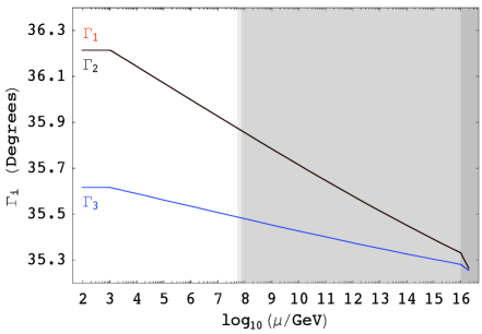
(a)

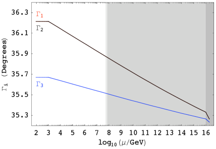
(b)

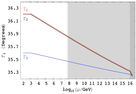
(c)

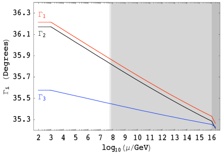
(d)

Figure 1: Evolution of sum rules $\Gamma_{1}$,$\Gamma_{2}$, $\Gamma_{3}$ for Cabibbo-like charged lepton corrections for large $\tan(\beta)=50$. Panel LABEL:sub@fig:sum shows the running at $\theta_{12}^{E}=5\,^{\circ}$ and $\lambda_{12}^{E}=0\,^{\circ}$, while panel LABEL:sub@fig:sumh shows the evolution at $\theta_{12}^{E}=8\,^{\circ}$ and $\lambda_{12}^{E}=0\,^{\circ}$. In panel LABEL:sub@fig:sumoo, the running is at $\theta_{12}^{E}=5\,^{\circ}$ and $\lambda_{12}^{E}=15\,^{\circ}$ while panel LABEL:sub@fig:sumff shows the evolution at $\theta_{12}^{E}=5\,^{\circ}$, $\lambda_{12}^{E}=30\,^{\circ}$. Note how the graphs for $\Gamma_{1}$ and $\Gamma_{2}$ completely overlap in LABEL:sub@fig:sum and LABEL:sub@fig:sumh.

(a)

(b)

Figure 2: Evolution of sum rules $\Gamma_{1}$, $\Gamma_{3}$ for Cabibbo-like charged lepton corrections for various $\tan(\beta)$. Running of $\Gamma_{1}$ is shown in panel LABEL:sub@fig:tanb and $\Gamma_{3}$ is shown in panel LABEL:sub@fig:tanb1 at $\theta_{12}^{E}=5\,^{\circ}$, $\lambda_{12}^{E}=0\,^{\circ}$ and different values of $\tan(\beta)$. Note the expanded (and different) vertical scales used in these two figures; in all cases the corrections are less than one degree.

5.1.2 Sum rules in terms of TB deviation parameters

In this subsection, for completeness we study the evolution of the TB deviation parameters defined in Eq.2.5. Their RG evolution, for different values of $\theta_{12}^{E}$, is shown in Fig.3. In Fig.4 we display the evolution of the sum rules given by Eqs.4.11, 4.12. From Fig.4 it is seen that both $\sigma_{1}$, $\sigma_{2}$ are precisely equal to zero at the GUT scale for $\theta_{12}^{E}=0$ but differ by a tiny amount for $\theta_{12}^{E},\lambda_{12}^{E}\not=0$. In this numerical example it is apparent that the sum rule $\sigma_{2}$ is slightly more stable than the original sum rule $\sigma_{1}$, although there is not much more stability. This is a manifestation of the fact that $\sigma_{2}$ does not take into account the running of $r$, which introduces an effect coming from the Majorana phases which we have assumed to be zero in this example. Later on we shall discuss a numerical example with non-zero Majorana phases where the enhanced stability of $\sigma_{2}$ will be more pronounced.

(a)

(b)

Figure 3: Evolution of the deviation parameters $r$, $s$, $a$ from the GUT scale to the electroweak scale without and with charged lepton corrections for large $\tan(\beta)=50$. Panel LABEL:sub@fig:dev0 shows the running of the deviation parameters without any charged lepton corrections, $\theta_{12}^{E}=0\,^{\circ}$, $\lambda_{12}^{E}=0\,^{\circ}$. Panel LABEL:sub@fig:dev1 shows the running of the deviation parameters in the presence of Cabibbo-like charged lepton corrections, $\theta_{12}^{E}=5\,^{\circ}$, $\lambda_{12}^{E}=15\,^{\circ}$.

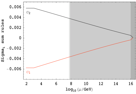
(a)

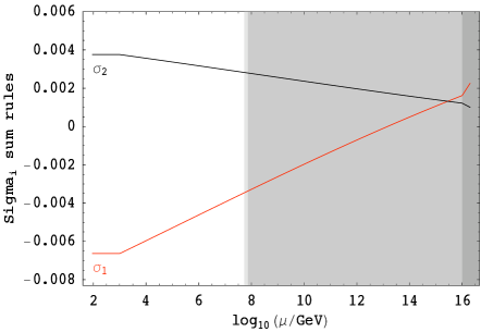
(b)

Figure 4: Evolution of the sum rules $\sigma_{1}$ and $\sigma_{2}$ from the GUT scale to the electroweak scale without and with charged lepton corrections for large $\tan(\beta)=50$. Panel LABEL:sub@fig:sdo shows the running without any charged lepton corrections, $\theta_{12}^{E}=0\,^{\circ}$ and $\lambda_{12}^{E}=0\,^{\circ}$. In panel LABEL:sub@fig:sdt the evolution is in the presence of Cabibbo-like charged lepton corrections, $\theta_{12}^{E}=5\,^{\circ}$ and $\lambda_{12}^{E}=30\,^{\circ}$

5.2 Sum rules with more general charged lepton corrections including $\theta_{23}^{E}$

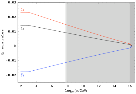
(a)

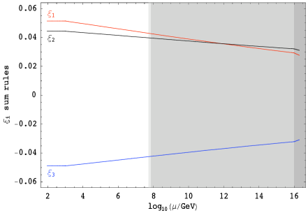
(b)

Figure 5: The evolution of the third row deviation parameters $\xi_{1}$, $\xi_{2}$ and $\xi_{3}$ from the GUT scale to the electroweak scale at $\tan(\beta)=50$ for Cabibbo-like and more general charged lepton corrections. Panel LABEL:sub@fig:xim1 shows the result with Cabibbo-like charged lepton corrections with $\theta_{23}^{E}=0\,^{\circ}$, $\lambda_{23}^{E}=0\,^{\circ}$, $\theta_{12}^{E}=5\,^{\circ}$ and $\lambda_{12}^{E}=30\,^{\circ}$. Panel LABEL:sub@fig:xim2 is for the case of more general charged lepton corrections with $\theta_{23}^{E}=2\,^{\circ}$ , $\lambda_{23}^{E}=30\,^{\circ}$, $\theta_{12}^{E}=5\,^{\circ}$ and $\lambda_{12}^{E}=30\,^{\circ}$.

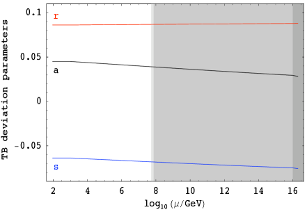
(a)

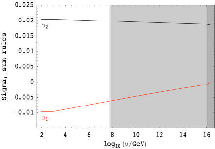
(b)

Figure 6: Running of the TB deviation parameters and their related sum rules from the GUT scale to the electroweak scale in the presence of more general charged lepton corrections, $\theta_{12}^{E}=5\,^{\circ}$, $\lambda_{12}^{E}=30\,^{\circ}$, $\lambda_{23}^{E}=30\,^{\circ}$, $\theta_{23}^{E}=2\,^{\circ}$ and $\tan(\beta)=50$. Panel LABEL:sub@fig:ns1 shows the evolution of the TB deviation parameters. Panel LABEL:sub@fig:ns2 displays the sum rules $\sigma_{1}$ and $\sigma_{2}$. Note that $\sigma_{1}=0$ at the GUT scale even in the presence of the more general charged lepton corrections.

Finally in this subsection we study the evolution of the $\xi_{i}$ parameters for the case of charged lepton corrections of the more general form in Eq.4.15. In Fig.5 LABEL:sub@fig:xim1 we show the RG running of the parameters $\xi_{1}$, $\xi_{2}$ and $\xi_{3}$, given in terms of the mixing angles in Eq. 2.9, for the case of Cabibbo-like charged lepton corrections. As expected, for Cabibbo-like charged lepton corrections, these parameters are exactly zero at the GUT scale for all values of $\theta_{12}^{E}$ and $\lambda_{12}^{E}$, but then diverge from zero due to the RG corrections. In Fig. 5 LABEL:sub@fig:xim2 we now switch on the non-Cabibbo-like charged lepton corrections by a small amount corresponding to $\theta_{23}^{E}=2\,^{\circ}$. In this case we see that the parameters $\xi_{1}$, $\xi_{2}$ and $\xi_{3}$ are all non zero at the GUT scale and deviate even more at low energies due to RG running.

In Fig.6 we show the running of the TB deviation parameters and the sum rules $\sigma_{1}$ and $\sigma_{2}$ for the non-Cabibbo-like case with $\theta_{23}^{E}=2\,^{\circ}$. It is clear from panel (b) that the $\sigma_{1}$ sum rule is still valid at the GUT scale even for a non-zero $\theta_{23}$, as remarked earlier.

5.3 Sum rules with non-zero Majorana phases

So far we have presented results for a particular example with zero Majorana phases. In this section, we present the running of the $\sigma_{i}$ sum rules and the TB deviation parameters where the neutrino Yukawa matrix is taken to be similar to Eq.4.13 with the same values for $b$, $e$ and $c_{3}$ but with non- zero Majorana phases:

$$Y_{LR}^{\nu}=\left(\begin{array}[]{ccc}0&0.97282be^{i\delta_{2}}&0.001\\ ee^{i\delta_{1}}&be^{i\delta_{2}}&0\\ -1.012ee^{i\delta_{1}}&be^{i\delta_{2}}&c_{3}\end{array}\right)$$ (5.1)

where we shall take the phases to be $\delta_{1}=120^{o}$ and $\delta_{2}=60^{o}$. The right-handed Majorana mass matrix is as before. The numerical value of the Yukawa couplings has been changed slightly to compensate for the non-zero phases in order to once again yield exact tri-bimaximal neutrino mixing at the GUT scale.

In Fig. 7 we show results for the running of the sum rules $\sigma_{i}$ and for the deviation parameters $r,s,a$ for the above example with non-zero Majorana phases. In this example the $\sigma_{2}$ sum rule is much more stable than $\sigma_{1}$ as clearly shown in Fig.7 LABEL:sub@fig:news. This shows that the question of the stability of the sum rule $\sigma_{2}$ is dependent on the choice of Majorana phases via the running of $r$. In particular with this choice of Majorana phases the deviation parameters $s$, $a$ and $r$ all run less as shown in Fig.7 LABEL:sub@fig:newdev, compared to the previous case with zero phases (Fig.3 LABEL:sub@fig:dev0 ).

The $\Gamma_{i}$ and $\xi_{i}$ sum rules also change with the Majorana phases turned on but not as much as $\sigma_{i}$ sum rules. For instance, at $\theta_{12}^{E}=5^{o}$ and $\lambda_{12}^{E}=0^{o}$, we find that $\Gamma_{1}$ and $\Gamma_{2}$ get smaller by 0.05 degrees at the $M_{Z}$ scale compared to the case where the phases are zero. $\Gamma_{3}$ on the other hand gets larger by about 0.1 degrees. At $\theta_{12}^{E}=5^{o}$ and $\lambda_{12}^{E}=30^{o}$, $\xi_{1}$ and $\xi_{2}$ get smaller by about 0.001 to 0.003 compared to the zero phases case whereas $\xi_{3}$ gets larger by 0.006.

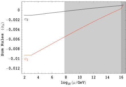
(a)

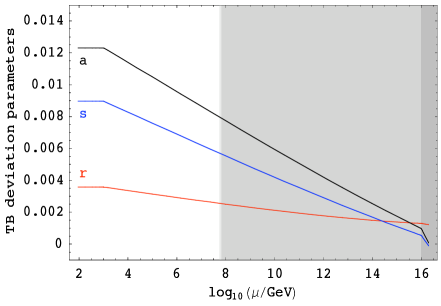
(b)

Figure 7: Sum rules with Majorana phases. The running of $\sigma_{i}$ sum rules and TB deviation parameters are for $\theta_{12}^{E}=0\,^{\circ}$, $\lambda_{12}^{E}=0\,^{\circ}$, $\tan(\beta)=50$, $\delta_{1}=120^{o}$ and $\delta_{2}=60^{o}$.

6 Model dependence of the results: heavy sequential dominance

So far all the numerical results have been based on a particular example inspired by the models of [2, 6], namely the case where the GUT scale neutrino Yukawa matrix has the form in Eq.4.13, or the closely related form in Eq.5.1 with non-zero Majorana phases. In these examples the dominant contribution to atmospheric neutrino mass is coming from the lightest right-handed neutrino via the see-saw mechanism, a situation known as light sequential dominance (LSD) [18]. In order to test the generality of the results in this section we consider a quite different example in which the dominant contribution to the atmospheric neutrino mass is coming from the heaviest right-handed neutrino via the see-saw mechanism, a situation known as heavy sequential dominance (HSD) [18]. This example is chosen since it the most qualitatively different to the example of LSD considered previously, yet despite this we shall see that the numerical results for the corrections to TB mixing are qualitatively similar to those encountered previously. This gives us some confidence that our results and conclusions are not restricted to the particular numerical example studied but are in fact applicable to a large class of see-saw models based on hierarchical neutrino masses.

In the HSD example considered here the right handed neutrino Majorana matrix as well as the neutrino Yukawa matrix are given by the following equations:

$$M_{RR}=\left(\begin{array}[]{ccc}3.991\times 10^{-6}&0&0\\ 0&5.800\times 10^{-4}&0\\ 0&0&5.021\end{array}\right)M_{3},$$

where $M_{3}=10^{14}GeV$. Ignoring RGE corrections to begin with, we find that precise tri-bimaximal neutrino mixing at the GUT scale ($\theta^{\nu}_{12}=35.26\,^{\circ}$, $\theta^{\nu}_{23}=45.00\,^{\circ}$, $\theta^{\nu}_{13}=0.00\,^{\circ}$) can be achieved with the Yukawa matrix:

$$Y_{LR}^{\nu}=\left(\begin{array}[]{ccc}1.001\times 10^{-7}&1.0036~{}b&0\\ 0&b&-1.0013~{}e\\ 2.992\times 10^{-5}&b&e\end{array}\right)$$ (6.1)

where $b~{}=2.401\times 10^{-3}$, $e~{}=0.677$. These parameters also lead to the following values for the neutrino masses: $\Delta m^{2}_{atm}=2.47\times 10^{-3}eV^{2}$ and $\Delta m^{2}_{sol}=7.53\times 10^{-5}eV^{2}$ which are well within the allowed experimental ranges.

Note that in the case of HSD the Yukawa couplings present in the neutrino Yukawa matrix are larger than the previous case especially $e$ which we take to be 0.677 compared to $2.125\times 10^{-4}$ in the previous example. Furthermore there are similarly two large Yukawa couplings in the third column of the Yukawa matrix. Moreover the heaviest RH neutrino associated with these large Yukawa couplings has a mass well below the GUT scale leading larger threshold corrections coming from it.

We assume charged lepton corrections of the form of Eq.4.1, the neutrino Yukawa matrix in the non-diagonal charged lepton basis is then transformed to the diagonal charged lepton basis according to Eq.4.14. Using the REAP package, the running of $\Gamma_{i}$ sum rules was performed from the GUT scale to low energy scale and the results are shown in Figure.8. As shown in this figure, despite the larger threshold corrections, for $\tan(\beta)=50$, the RG running of $\Gamma_{3}$ is still small (about $0.4^{o}$) whereas that of $\Gamma_{1}$ and $\Gamma_{2}$ is about $1.3^{o}$, compared to the results shown in Figure.2 (nearly $1^{o}$). This suggests that, qualitatively, the results obtained for the previous numerical example inspired by the GUT models in [2, 6] are expected to have wide applicability beyond the specific example considered.

(a)

(b)

(c)

Figure 8: Sum rules with heavy sequential dominance. This figure shows the evolution of the $\Gamma_{i}$ sum rules for $\tan\beta=50$ (panel LABEL:sub@fig:nm1), the running of $\Gamma_{1}$ and $\Gamma_{3}$ in terms of $\tan\beta$ (panels LABEL:sub@fig:nm2, LABEL:sub@fig:nm3) from the GUT scale to the electroweak scale for the case of Cabibbo-like charged lepton corrections with $\theta_{12}^{E}=5\,^{\circ}$, $\lambda_{12}^{E}=0\,^{\circ}$.

7 Justification of the numerical approach

The results in this paper have been based on a numerical evaluation of the RG corrections using the REAP package. The reasons why we have chosen to study these corrections numerically, rather than using analytic estimates [17] are as follows.

The first reason we follow the numerical approach is that, as we show, some analytic estimates of RG effects which have ignored the effects of phases are unreliable. For example, the main purpose of this paper is to find out precisely how large the RG corrections are to sum rule relations which have been proposed in the literature (see section 4.1.1). Although the RG corrections to such sum rules are expected to be small, they are certainly not negligible compared to the expected precision of future neutrino experiments, and indeed this prompted the introduction of the modified sum rule in Eq.4.12, where the extra term compared to Eq.4.11 was supposed to take into account the RG corrections [19]. However, it turns out that the new analytic term, which ignores the effects of phases, is too simplistic. Indeed the numerical results in Figures 4a and 7a clearly show that the extra term included in the analytic estimate of the RG correction in Eq.4.12 does not capture the phase dependence of the RG correction to the original sum rule in Eq.4.11. The numerical study in this paper has highlighted the shortcoming of analytic estimates of the RG corrections to sum rules which do not include the phase dependence.

The second reason we follow the numerical approach, rather than an analytic approach, is that for some of the cases studied the analytic approach is simply not applicable. The usual analytic approach is based on the assumption that only the third family charged lepton and neutrino Yukawa couplings are taken into account (while many analytic studies ignore neutrino Yukawa couplings and threshold effects altogether). Whilst the approximation of keeping only third family Yukawa couplings is sufficient for some models, for example the LSD class of models, it is certainly not sufficient for all classes of models. For example the HSD case that we also study involves two large neutrino Yukawa couplings, and the analytic estimates in [19] do not directly apply to this case.

The third reason for following a numerical approach is a purely quantitative one, namely, even for the cases where the analytic approach is reliable and applicable (and we have already seen examples in the previous two paragraphs when it is neither) we would like to obtain the best possible estimate of the RG corrections which are the main focus of this paper. If the sum rules are to be confronted with experiment, it is important to have a reliable quantitative handle on the RG corrections, and for this purpose it is necessary to go beyond the leading log analytic approximation, as we now discuss.

In order to investigate the quantitative accuracy of the analytic approach, in the remainder of this section we shall compare the analytic estimates of the RG effects for the LSD example studied earlier in the paper. For this purpose it is sufficient to switch off the charged lepton corrections and study the RG corrections to the neutrino mixing angles using the analytic approximations in [17] which we then compare to the numerical results we obtained earlier in the paper, and which we also summarize here for convenience. In order to estimate the RG corrections to the mixing angles, following [17] it is assumed that the (3,3) matrix elements govern both the charged Yukawa matrix ($Y^{e}$) and the neutrino Yukawa matrix ($Y^{\nu}$) in the flavour basis in which the charged lepton mass matrix is diagonal. Taking $Y^{e}\approx diag(0,0,y_{\tau})$ and $Y^{\nu}\approx diag(0,0,y_{\nu_{3}})$, one finds, to leading log approximation, that there is a single parameter which governs the RG corrections to all the mixing angles given by [19]:

$$\eta^{RG}=\frac{y_{\tau}^{2}}{8\pi^{2}}\ln\frac{M_{GUT}}{M_{Z}}+\frac{y_{\nu_{3}}^{2}}{8\pi^{2}}\ln\frac{M_{GUT}}{M_{3}}.$$ (7.1)

Assuming tri-bimaximal neutrino mixing at the GUT scale, the low energy scale parameters are then given approximately by:

$$s_{12}^{\nu}(M_{Z})=\frac{1}{\sqrt{3}}(1+\frac{\eta^{RG}}{6})~{}~{},~{}~{}s_{23}^{\nu}(M_{Z})=\frac{1}{\sqrt{2}}(1+\frac{\eta^{RG}}{4})~{}~{},~{}~{}s_{13}^{\nu}(M_{Z})=\frac{\eta^{RG}}{3}\frac{m_{2}}{m_{3}}.$$ (7.2)

We now apply the above analytic formalism to the LSD model defined in section.4.1.2, and subsequently studied numerically in this paper. In this model from Eq.4.13 we see that $y_{\nu_{3}}=c_{3}=0.58$ at the GUT scale. We also find $y_{\tau}=0.33$ and the mass ratio $m_{2}/m_{3}=0.16$ for the case $\tan(\beta)=50$. Using these values, the mixing angles and the quantities ($\Gamma_{i}$) can be estimated as shown in Table.7, where the analytic estimates are shown alongside the numerical results for comparison.

Parameter	$\theta_{12}^{\nu}$	$\theta_{23}^{\nu}$	$\theta_{13}^{\nu}$	$\Gamma_{1}$	$\Gamma_{2}$	$\Gamma_{3}$
Analytic (o)	35.59	45.69	0.15	35.94	35.94	35.44
Numerical (o)	35.65	46.00	0.15	36.21	36.21	35.49

Table 7: This table shows a comparison between the analytic and numerical results for the RG corrections to neutrino mixing angles at the $M_{Z}$ scale, assuming that they take the precise TB mixing values at the GUT scale, for the LSD model described in the body of the paper with $\tan(\beta)=50$.

It is interesting to compare the analytic results to the numerical results in Table 7 for the neutrino mixing angles at the $M_{Z}$ scale, assuming that they take the precise TB mixing values at the GUT scale and setting all charged lepton corrections to zero, for the LSD model described above. The results show that the numerical estimate of $\theta_{13}^{\nu}$ (which is equal to zero at the GUT scale) is very accurately reproduced by the analytic approximation (indeed there is no difference to 2 d.p.), and the RG correction to $\theta_{12}^{\nu}$ is also well reproduced with the analytic estimate underestimating the correction by only $0.06$ degrees. However the results also show that there is a significant underestimate of $\theta_{23}^{\nu}$ with the analytically estimated value at the $M_{Z}$ scale being less than the numerical value by about $0.3$ degrees, resulting in the analytically estimated values for $\Gamma_{1}$ and $\Gamma_{2}$ being less than the numerical values by about the same amount ($0.3^{o}$). From the point of view of the effects studied in this paper (for example note the precision of the scales shown in the results in Figure 1a) an error of $0.3$ degrees is undesirable and we would not wish to compromise the results in this paper by being subject to such unnecessary errors incurred by the analytic approach.

Finally we remark that the origin of the discrepancy between the analytic estimates and the numerical results, for the cases where the analytic approach is reliable and applicable, is due to the fact that the analytic estimates are based on the assumption that the Yukawa couplings $y_{\tau}$ and $y_{\nu_{3}}$ are fixed at their GUT scale values and do not run, whereas the numerical results allow for the co-running of all the Yukawa couplings in the matrix (including the second family Yukawa couplings), with the leading logs being effectively re-summed.

8 Summary and Conclusions

In this paper we have analyzed the effects of charged lepton corrections and RG running on the low energy predictions of theories which accurately predict tri-bimaximal neutrino mixing at the high energy scale. In GUT motivated examples the charged lepton corrections are often Cabibbo-like and in this case the effect of charged lepton corrections leads to a range of neutrino mixing sum rules at the GUT scale, given by the $\Gamma_{i}$ sum rules in Eqs.4.8,4.9,4.10, as well as the $\sigma_{i}$ sum rules expressed in terms of the deviation parameters in Eqs.4.11 and 4.12. We have studied the RG running of such sum rules numerically for a specific numerical example inspired by the GUT models in [2, 6], corresponding closely to CSD with LSD. Our results indicate small but measurable effects for the two examples studied. For example the $\Gamma_{3}$ sum rule arising from Cabibbo-like charged lepton corrections (due to $\theta_{12}^{E}$ corrections) which at the GUT scale corresponds to $\theta_{12}-\theta_{13}\cos(\delta)\approx 35.3^{o}$ becomes renormalized by about $0.4^{o}$ even for large $\tan\beta=50$. We have also considered the effect on charged lepton corrections coming from non-Cabibbo-like charged lepton corrections (due to non-zero $\theta_{23}^{E}$) and confirmed that the sum rule $\sigma_{1}$ is insensitive to $\theta_{23}^{E}$.

Even for a particular class of numerical model, such as the GUT-flavour inspired LSD model considered, the numerical results will depend in general on the choice of Majorana phases for that model. We have seen that switching on these Majorana phases can alter significantly the running of the TB mixing deviation parameters $r,s,a$ as well as the sum rules such as $\sigma_{i}$. For example the sum rule $\sigma_{2}$ which includes the leading logarithmic RG corrections due to the running of $s$ and $a$, will have a Majorana phase dependence via the running of $r$ which was neglected in the derivation of $\sigma_{2}$ [19]. Thus, the relative stability of $\sigma_{2}$ as compared to $\sigma_{1}$ turns out to be a Majorana phase dependent question.

Although most of the numerical results are based on a particular GUT-flavour motivated LSD type of model, we have also considered similar results for a completely different type of model based on HSD. Overall we have found that the RG running effects are quite small in both cases which suggests that qualitatively similar results will apply to other models based on the Minimal Supersymmetric Standard Model, extended to include the see-saw mechanism, with hierarchical neutrino masses. However, we repeat our caveat in the Introduction that in this paper we have only considered deviations from TB lepton mixing due to the combination of charged lepton corrections and RG running, and that in general there will be other sources of deviations that we do not consider. For example, exact CSD [2] itself will lead to some deviations since it does not predict precisely TB neutrino mixing due to corrections of order $m_{2}/m_{3}$ [18]. Another example of deviations to TB mixing are the canonical normalization effects discussed in [19]. In general corrections to the TB mixing in the neutrino sector, in the flavour basis, are highly model dependent and have been studied phenomenologically in [20].

Finally we note that all the results in this paper are based on a numerical approach rather than an analytic approach. We have given three reasons to justify the use of the numerical approach: firstly that analytic results which ignore the effects of phases are not reliable (for example the $\sigma_{2}$ sum rule); secondly that analytic results may not be applicable for all cases of interest (for example HSD with two large neutrino Yukawa couplings); and thirdly that the quantitative precision of the analytic approach is not in general sufficient for our purpose here (in particular we have shown that the RG correction to $\theta_{23}$ may be significantly underestimated in the analytic approach). Therefore throughout this paper we have adopted a numerical approach, exploiting the convenient REAP package.

To conclude, we have assumed precise TB neutrino mixing at the GUT scale, and investigated the deviations due to both charged lepton corrections and RG running. In GUT-flavour inspired models the charged lepton corrections are expected to resemble those of the quark mixing matrix, and lead to neutrino mixing sum rules which are valid at high energy. We have studied numerically a variety of such neutrino mixing sum rules and shown that, in the types of GUT-flavour models in which the sum rules emerge in the first place, they are subject to only mild RG corrections (less than one degree for the cases studied) in evolving them down to low energy. However even such small corrections as described in this paper will nevertheless be important when comparing the neutrino mixing sum rules to the results of future high precision neutrino oscillation experiments [34].

References

- [1] P. F. Harrison, D. H. Perkins and W. G. Scott, Phys. Lett. B 530 (2002) 167 [arXiv:hep-ph/0202074]; P. F. Harrison and W. G. Scott, Phys. Lett. B 535 (2002) 163 [arXiv:hep-ph/0203209]; P. F. Harrison and W. G. Scott, Phys. Lett. B 557 (2003) 76 [arXiv:hep-ph/0302025]; see also L. Wolfenstein, Phys. Rev. D 18 (1978) 958.
- [2] S. F. King, JHEP 0508 (2005) 105 [arXiv:hep-ph/0506297].
- [3] P. H. Frampton, S. T. Petcov and W. Rodejohann, Nucl. Phys. B 687 (2004) 31 [arXiv:hep-ph/0401206]; F. Plentinger and W. Rodejohann, Phys. Lett. B 625 (2005) 264 [arXiv:hep-ph/0507143]; R. N. Mohapatra and W. Rodejohann, Phys. Rev. D 72 (2005) 053001 [arXiv:hep-ph/0507312]; K. A. Hochmuth, S. T. Petcov and W. Rodejohann, arXiv:0706.2975 [hep-ph]; T. Ohlsson and G. Seidl, Nucl. Phys. B 643 (2002) 247 [arXiv:hep-ph/0206087];
- [4] G. Altarelli, F. Feruglio and Y. Lin, Nucl. Phys. B 775 (2007) 31 [arXiv:hep-ph/0610165]; G. Altarelli and F. Feruglio, Nucl. Phys. B 741 (2006) 215 [arXiv:hep-ph/0512103]; G. Altarelli and F. Feruglio, Nucl. Phys. B 720 (2005) 64 [arXiv:hep-ph/0504165]; F. Feruglio, C. Hagedorn, Y. Lin and L. Merlo, Nucl. Phys. B 775 (2007) 120 [arXiv:hep-ph/0702194]. C. Luhn, S. Nasri and P. Ramond, Phys. Lett. B 652 (2007) 27 [arXiv:0706.2341 [hep-ph]]; F. Plentinger and G. Seidl, Phys. Rev. D 78 (2008) 045004 [arXiv:0803.2889 [hep-ph]]; C. Csaki, C. Delaunay, C. Grojean and Y. Grossman, arXiv:0806.0356 [hep-ph].
- [5] E. Ma, arXiv:0709.0507 [hep-ph]; E. Ma, arXiv:hep-ph/0701016; E. Ma, Mod. Phys. Lett. A 22 (2007) 101 [arXiv:hep-ph/0610342]; E. Ma, Mod. Phys. Lett. A 21 (2006) 2931 [arXiv:hep-ph/0607190]; E. Ma, Mod. Phys. Lett. A 21 (2006) 1917 [arXiv:hep-ph/0607056]; E. Ma, H. Sawanaka and M. Tanimoto, Phys. Lett. B 641 (2006) 301 [arXiv:hep-ph/0606103]; E. Ma, Phys. Rev. D 73 (2006) 057304; B. Adhikary, B. Brahmachari, A. Ghosal, E. Ma and M. K. Parida, Phys. Lett. B 638 (2006) 345 [arXiv:hep-ph/0603059]; E. Ma, Mod. Phys. Lett. A 20 (2005) 2601 [arXiv:hep-ph/0508099]; E. Ma, Phys. Rev. D 72 (2005) 037301 [arXiv:hep-ph/0505209]; S. L. Chen, M. Frigerio and E. Ma, Nucl. Phys. B 724 (2005) 423 [arXiv:hep-ph/0504181]; E. Ma, Phys. Rev. D 70 (2004) 031901 [arXiv:hep-ph/0404199].
- [6] I. de Medeiros Varzielas and G. G. Ross, Nucl. Phys. B 733 (2006) 31 [arXiv:hep-ph/0507176]; I. de Medeiros Varzielas, S. F. King and G. G. Ross, Phys. Lett. B 644 (2007) 153 [arXiv:hep-ph/0512313]; I. de Medeiros Varzielas, S. F. King and G. G. Ross, Phys. Lett. B 648 (2007) 201 [arXiv:hep-ph/0607045];
- [7] S. F. King and M. Malinsky, Phys. Lett. B 645 (2007) 351 [arXiv:hep-ph/0610250]; S. F. King and M. Malinsky, JHEP 0611 (2006) 071 [arXiv:hep-ph/0608021];
- [8] P. F. Harrison and W. G. Scott, Phys. Lett. B 557 (2003) 76 [arXiv:hep-ph/0302025]; P. F. Harrison and W. G. Scott, Phys. Lett. B 535 (2002) 163 [arXiv:hep-ph/0203209]; R. N. Mohapatra, S. Nasri and H. B. Yu, Phys. Lett. B 639 (2006) 318 [arXiv:hep-ph/0605020]; R. N. Mohapatra and H. B. Yu, Phys. Lett. B 644 (2007) 346 [arXiv:hep-ph/0610023]; M. C. Chen and K. T. Mahanthappa, Phys. Lett. B 652 (2007) 34 [arXiv:0705.0714 [hep-ph]]; C. I. Low and R. R. Volkas, Phys. Rev. D 68 (2003) 033007 [arXiv:hep-ph/0305243]; X. G. He, Nucl. Phys. Proc. Suppl. 168 (2007) 350 [arXiv:hep-ph/0612080]; A. Aranda, arXiv:0707.3661 [hep-ph].
- [9] A. H. Chan, H. Fritzsch and Z. z. Xing, arXiv:0704.3153 [hep-ph]; Z. z. Xing, Phys. Lett. B 618 (2005) 141 [arXiv:hep-ph/0503200]; Z. z. Xing, H. Zhang and S. Zhou, Phys. Lett. B 641 (2006) 189 [arXiv:hep-ph/0607091]; S. K. Kang, Z. z. Xing and S. Zhou, Phys. Rev. D 73 (2006) 013001 [arXiv:hep-ph/0511157]; S. Luo and Z. z. Xing, Phys. Lett. B 632 (2006) 341 [arXiv:hep-ph/0509065]; M. Hirsch, E. Ma, J. C. Romao, J. W. F. Valle and A. Villanova del Moral, Phys. Rev. D 75 (2007) 053006 [arXiv:hep-ph/0606082]; N. N. Singh, M. Rajkhowa and A. Borah, arXiv:hep-ph/0603189; X. G. He and A. Zee, Phys. Lett. B 645 (2007) 427 [arXiv:hep-ph/0607163]; N. Haba, A. Watanabe and K. Yoshioka, Phys. Rev. Lett. 97 (2006) 041601 [arXiv:hep-ph/0603116].
- [10] S. Antusch, L. E. Ibanez and T. Macri, JHEP 0709 (2007) 087.
- [11] E. Ma and G. Rajasekaran, Phys. Rev. D 64 (2001) 113012 [arXiv:hep-ph/0106291].
- [12] Z. z. Xing, Phys. Lett. B 533 (2002) 85 [arXiv:hep-ph/0204049].
- [13] I. Masina, Phys. Lett. B 633 (2006) 134 [arXiv:hep-ph/0508031].
- [14] S. Antusch and S. F. King, Phys. Lett. B 631 (2005) 42 [arXiv:hep-ph/0508044]; S. Antusch, P. Huber, S. F. King and T. Schwetz, JHEP 0704 (2007) 060 [arXiv:hep-ph/0702286].
- [15] P. H. Chankowski and Z. Pluciennik, Phys. Lett. B316 (1993), 312–317, hep-ph/9306333; K. S. Babu, C. N. Leung, and J. Pantaleone, Phys. Lett. B319 (1993), 191–198, hep-ph/9309223; N. Haba, N. Okamura and M. Sugiura, Prog. Theor. Phys. 103 (2000) 367 [arXiv:hep-ph/9810471]; N. Haba, Y. Matsui, N. Okamura and M. Sugiura, Eur. Phys. J. C 10 (1999) 677 [arXiv:hep-ph/9904292]; N. Haba and N. Okamura, Eur. Phys. J. C 14 (2000) 347 [arXiv:hep-ph/9906481]; N. Haba, Y. Matsui, N. Okamura and M. Sugiura, Prog. Theor. Phys. 103 (2000) 145 [arXiv:hep-ph/9908429]; N. Haba, Y. Matsui and N. Okamura, Eur. Phys. J. C 17 (2000) 513 [arXiv:hep-ph/0005075]; N. Haba, Y. Matsui and N. Okamura, Prog. Theor. Phys. 103 (2000) 807 [arXiv:hep-ph/9911481]; S. Antusch, M. Drees, J. Kersten, M. Lindner, and M. Ratz, Phys. Lett. B519 (2001), 238–242, hep-ph/0108005; S. F. King and N. N. Singh, Nucl. Phys. B591 (2000), 3–25, hep-ph/0006229; S. Antusch and M. Ratz, JHEP 11 (2002), 010, hep-ph/0208136; P. H. Chankowski, W. Krolikowski, and S. Pokorski, Phys. Lett. B473 (2000), 109, hep-ph/9910231; J. A. Casas, J. R. Espinosa, A. Ibarra, and I. Navarro, Nucl. Phys. B573 (2000), 652, hep-ph/9910420; S. Antusch, J. Kersten, M. Lindner, and M. Ratz, Nucl. Phys. B674 (2003), 401–433, hep-ph/0305273.
- [16] S. Antusch, J. Kersten, M. Lindner and M. Ratz, Phys. Lett. B 544 (2002) 1 [arXiv:hep-ph/0206078].
- [17] S. Antusch, J. Kersten, M. Lindner, M. Ratz and M. A. Schmidt, JHEP 0503 (2005) 024 [arXiv:hep-ph/0501272].
- [18] S. F. King, Phys. Lett. B 439 (1998) 350 [arXiv:hep-ph/9806440]; S. F. King, Nucl. Phys. B 562 (1999) 57 [arXiv:hep-ph/9904210]; S. F. King, Nucl. Phys. B 576 (2000) 85 [arXiv:hep-ph/9912492]; S. F. King, JHEP 0209 (2002) 011 [arXiv:hep-ph/0204360]. For a review, see: S. Antusch and S. F. King, New J. Phys. 6 (2004) 110 [arXiv:hep-ph/0405272];
- [19] S. Antusch, S. F. King and M. Malinsky, arXiv:0711.4727 [hep-ph]; S. Antusch, S. F. King and M. Malinsky, JHEP 0805 (2008) 066 [arXiv:0712.3759 [hep-ph]].
- [20] C. H. Albright and W. Rodejohann, arXiv:0804.4581 [hep-ph].
- [21] S. Luo and Z. z. Xing, Phys. Lett. B 632 (2006) 341 [arXiv:hep-ph/0509065]; A. Dighe, S. Goswami and W. Rodejohann, Phys. Rev. D 75 (2007) 073023 [arXiv:hep-ph/0612328].
- [22] T. Schwetz, AIP Conf. Proc. 981 (2008) 8 [arXiv:0710.5027 [hep-ph]].
- [23] M. Maltoni, T. Schwetz, M. A. Tortola and J. W. F. Valle, Phys. Rev. D 68 (2003) 113010 [arXiv:hep-ph/0309130].
- [24] M. Maltoni, T. Schwetz, M. A. Tortola and J. W. F. Valle, New J. Phys. 6 (2004) 122 [arXiv:hep-ph/0405172].
- [25] S. F. King, Phys. Lett. B 659 (2008) 244 [arXiv:0710.0530 [hep-ph]].
- [26] S. F. King, arXiv:0712.1750 [hep-ph].
- [27] P. Minkowski, Phys. Lett. B 67 (1977) 421; M. Gell-Mann, P. Ramond and R. Slansky in Sanibel Talk, CALT-68-709, Feb 1979, and in Supergravity (North Holland, Amsterdam 1979); T. Yanagida in Proc. of the Workshop on Unified Theory and Baryon Number of the Universe, KEK, Japan, 1979; S.L.Glashow, Cargese Lectures (1979); R. N. Mohapatra and G. Senjanovic, Phys. Rev. Lett. 44 (1980) 912; J. Schechter and J. W. Valle, Phys. Rev. D 25 (1982) 774.
- [28] S. Antusch and S. F. King, New J. Phys. 6 (2004) 110 [arXiv:hep-ph/0405272].
- [29] G. Lazarides, Q. Shafi and C. Wetterich, Nucl. Phys. B 181 (1981) 287.
- [30] S. F. King, JHEP 0209 (2002) 011 [arXiv:hep-ph/0204360].
- [31] S. F. King, Phys. Rev. D 67 (2003) 113010 [arXiv:hep-ph/0211228].
- [32] Charged lepton contributions to neutrino mixings have been considered, e.g., in: P. H. Frampton, S. T. Petcov and W. Rodejohann, Nucl. Phys. B 687 (2004) 31, hep-ph/0401206; G. Altarelli, F. Feruglio and I. Masina, Nucl. Phys. B 689 (2004) 157, hep-ph/0402155; S. Antusch and S. F. King, Phys. Lett. B 591 (2004) 104, hep-ph/0403053; F. Feruglio, Nucl. Phys. Proc. Suppl. 143 (2005) 184 [Nucl. Phys. Proc. Suppl. 145 (2005) 225], hep-ph/0410131; R. N. Mohapatra and W. Rodejohann, hep-ph/0507312.
- [33] S. Antusch and S. F. King, Phys. Lett. B 659 (2008) 640 [arXiv:0709.0666 [hep-ph]].
- [34] A. Bandyopadhyay et al. [ISS Physics Working Group], arXiv:0710.4947 [hep-ph].