Unifying practical uncertainty representations: II. Clouds

Abstract.

There exist many simple tools for jointly capturing variability and incomplete information by means of uncertainty representations. Among them are random sets, possibility distributions, probability intervals, and the more recent Ferson’s p-boxes and Neumaier’s clouds, both defined by pairs of possibility distributions. In the companion paper, we have extensively studied a generalized form of p-box and situated it with respect to other models . This paper focuses on the links between clouds and other representations. Generalized p-boxes are shown to be clouds with comonotonic distributions. In general, clouds cannot always be represented by random sets, in fact not even by $2$-monotone (convex) capacities.

1. Introduction

There exist many different tools for representing imprecise probabilities. Usually, the more general, the more difficult they are to handle. Simpler representations, although less expressive, usually have the advantage of being more tractable. Over the years, several such representations have been proposed. Among them are possibility distributions [22], probability intervals [5], and more recently p-boxes [14] and clouds [17, 18]. Comparing their respective expressive power is a natural task. Finding formal relations between such representations also facilitates a unified handling of uncertainty.

In the first part of paper [7], a generalized notion of p-boxes is studied and related to representations mentioned above. It is shown that any generalized p-box is representable by a pair of possibility distributions, and that generalized p-boxes are special cases of random sets. Their interpretation in terms of lower and upper confidence bounds on a collection of nested subsets makes them intuitive simple representations. Figure 1 recalls the connections established in the companion paper between the studied representations, going from the most (top) to the least (bottom) general.

Figure 1. Relationships among representations. $A\longrightarrow B$ A generalizes B. $A\dashrightarrow B$: B is representable by A

The present paper completes Figure 1 by adding clouds to it, making one step further towards the unification of uncertainty models. Clouds, encoded by a pair of fuzzy sets, were recently introduced by Neumaier [17] as a means to cope with imprecision while remaining computationally tractable, even in high dimensional spaces. Recently, Fuchs and Neumaier [15] have applied clouds to space shuttle design problem, demonstrating some of the potential of the representation. Moreover, as clouds are syntactically equivalent to interval-valued fuzzy sets with some boundary conditions, analyzing their connection with respect to other uncertainty theories also provides some insight about how interval-valued fuzzy sets can be interpreted by such theories. As we shall see, generalized p-boxes, studied in the companion paper, constitute a bridge between clouds, possibility distributions and usual p-boxes.

The paper is divided into five main sections; Section 2 studies the formalism of clouds and relates them to pairs of possibility distributions and to generalized p-boxes. It is shown that generalized p-boxes are equivalent to a particular subfamily of clouds, named here comonotonic clouds. Section 3 studies non-comonotonic clouds. Since the lower probability they induce are in general even not 2-monotone, simpler outer and inner approximations are proposed; Section 4 then studies relations between clouds and probability intervals. As neither of them is a special case of the other, some transformations of probability intervals into outer-approximating clouds are proposed. Section 5 extends some of our results to the case of continuous models defined on the real line, since such models are often encountered in applications. The particular case of thin clouds, for which both upper and lower distributions coincide is emphasized, as they have non-empty credal sets in the continuous setting.

To make the paper easier to read, longer proofs have been moved to the appendix. We will often refer to useful results from the companion paper [7], where basics about other representations and uncertainty theories considered here can be found. Some definitions are recalled in footnotes. In the first four sections, we consider that our uncertainty concerns the value that a variable could assume on a finite set $X$ containing $n$ elements.

2. Clouds

Clouds were introduced by Neumaier [17] as a probabilistic generalizations of intervals.

Definition 1.

A cloud $[\delta,\pi]$ is defined as a pair of mappings $\delta:X\to[0,1]$ and $\pi:X\to[0,1]$ from the set $X$ to the unit interval $[0,1]$, such that

• $\delta$ is pointwise less than or equal to $\pi$ (i.e. $\delta\leq\pi$),

• $\pi(x)=1$ for at least one element $x$ in $X$,

• $\delta(y)=0$ for at least one element $y$ in $X$.

$\delta$ and $\pi$ are respectively the lower and upper distributions of a cloud.

As mappings $\delta,\pi$ are mathematically equivalent to two nested fuzzy membership functions, a cloud $[\delta,\pi]$ is mathematically equivalent to an interval-valued fuzzy set (IVF)[21] with boundary conditions ($\pi(x)=1$ and $\delta(y)=0$). More precisely, it is mathematically equivalent to an interval-valued membership function whereby the membership value of each element $x$ of $X$ lies in $[\delta(x),\pi(x)]$. Since a cloud is equivalent to a pair of fuzzy membership functions, at most $2|X|-2$ values (notwithstanding boundary constraints on $\delta$ and $\pi$) are needed to fully determine a cloud on a finite set. Two subcases of clouds considered by Neumaier [17] are the thin and fuzzy clouds. A thin cloud is defined as a cloud for which $\delta=\pi$, while a fuzzy cloud is a cloud for which $\delta=0$.

Neumaier defines the credal set ${\mathcal{P}}_{[\delta,\pi]}$ induced by a cloud $[\delta,\pi]$, as:

(1) $${\mathcal{P}}_{[\delta,\pi]}\!=\!\{P\in{\mathbb{P}_{X}}|P(\{x\in X|\delta(x)\geq\alpha\})\leq 1-\alpha\leq P(\{x\in X|\pi(x)>\alpha\})\}$$

where ${\mathbb{P}_{X}}$ is the set of probability measures on $X$. Interestingly enough, this definition gives a mean to interpret IVF sets in terms of credal sets, or in terms of imprecise probabilities, eventually ending up with a behavioral interpretation of IVF by using Walley’s [20] theory of imprecise probabilities.

Let $0=\gamma_{0}<\gamma_{1}<\ldots<\gamma_{M}=1$ be the ordered distinct values taken by both $\delta$ and $\pi$ on elements of $X$, then denote the strong and regular cuts as

(2) $$B_{\overline{\gamma}_{i}}=\{x\in X|\pi(x)>\gamma_{i}\}\mbox{\leavevmode\nobreak\ and\leavevmode\nobreak\ }B_{\gamma_{i}}=\{x\in X|\pi(x)\geq\gamma_{i}\}$$

for the upper distribution $\pi$ and

(3) $$C_{\overline{\gamma}_{i}}=\{x\in X|\delta(x)>\gamma_{i}\}\mbox{\leavevmode\nobreak\ and\leavevmode\nobreak\ }C_{\gamma_{i}}=\{x\in X|\delta(x)\geq\gamma_{i}\}$$

for the lower distribution $\delta$. Note that in the finite case, $B_{\overline{\gamma}_{i}}=B_{\gamma_{i+1}}$ and $C_{\overline{\gamma}_{i}}=C_{\gamma_{i+1}}$, with $\gamma_{M+1}=1$, and also

$$\emptyset=B_{\overline{\gamma}_{M}}\subset B_{\overline{\gamma}_{M-1}}\subseteq\ldots\subseteq B_{\overline{\gamma}_{0}}=X;\quad\emptyset=C_{\gamma_{M}}\subseteq C_{\gamma_{M-1}}\subseteq\ldots\subseteq C_{\gamma_{0}}=X$$

and since $\delta\leq\pi$, this implies that $C_{\gamma_{i}}\subseteq B_{\gamma_{i}}$, hence $C_{\gamma_{i}}\subseteq B_{\overline{\gamma}_{i-1}}$, for all $i=1,\dots,M$. In such a finite case, a cloud is said to be discrete. In terms of constraints bearing on probabilities, the credal set ${\mathcal{P}}_{[\delta,\pi]}$ of a finite cloud is equivalently defined by the finite set of inequalities:

(4) $$i=0,\ldots,M,\quad P(C_{\gamma_{i}})\leq 1-\gamma_{i}\leq P(B_{\overline{\gamma}_{i}})$$

under the above inclusion constraints. Note that some conditions, in addition to boundary ones advocated in Definition 1, must hold for ${\mathcal{P}}_{[\delta,\pi]}$ to be non-empty in the finite case. In particular, distribution $\delta$ cannot be equal to $\pi$ (i.e. $\delta(x)\neq\pi$). Otherwise, we have $C_{\gamma_{i}}=B_{\overline{\gamma}_{i-1}}(=B_{\gamma_{i}})$, that is $\pi$ and $\delta$ have a common $\gamma_{i}$-cut, and there is no probability distribution satisfying the constraint $1-\gamma_{i-1}\leq P(C_{\gamma_{i}})\leq 1-\gamma_{i}$ since $\gamma_{i-1}<\gamma_{i}$. So, thin finite clouds induce empty credal sets.

Example 1.

This example illustrates the notion of a cloud and will be used in the next sections to illustrate various results. Let us consider a set $X=\{u,v,w,x,y,z\}$ and the following cloud $[\delta,\pi]$, pictured in Figure 2, defined on this set:

$$\begin{array}[]{c@{\hspace{10mm}}c@{\hspace{5mm}}c@{\hspace{5mm}}c@{\hspace{5mm}}c@{\hspace{5mm}}c@{\hspace{5mm}}c}\hfil\hskip 28.45274pt&u\hfil\hskip 14.22636pt&v\hfil\hskip 14.22636pt&w\hfil\hskip 14.22636pt&x\hfil\hskip 14.22636pt&y\hfil\hskip 14.22636pt&z\\ \hline\cr\pi\hfil\hskip 28.45274pt&0.75\hfil\hskip 14.22636pt&1\hfil\hskip 14.22636pt&1\hfil\hskip 14.22636pt&0.75\hfil\hskip 14.22636pt&0.75\hfil\hskip 14.22636pt&0.5\\ \delta\hfil\hskip 28.45274pt&0.5\hfil\hskip 14.22636pt&0.5\hfil\hskip 14.22636pt&0.75\hfil\hskip 14.22636pt&0.5\hfil\hskip 14.22636pt&0\hfil\hskip 14.22636pt&0\\ \hline\cr\end{array}$$

The values $\gamma_{i}$ corresponding to this cloud are

$$0\leq 0.5\leq 0.75\leq 1$$

$$\gamma_{0}\leq\gamma_{1}\leq\gamma_{2}\leq\gamma_{3}.$$

Constraints associated to this cloud and corresponding to Equation (4) are

$$P(C_{\gamma_{3}}=\emptyset) \leq 1-1\leq P(B_{\overline{\gamma}_{3}}=\emptyset)$$

$$P(C_{\gamma_{2}}=\{w\}) \leq 1-0.75\leq P(B_{\overline{\gamma}_{2}}=\{v,w\})$$

$$P(C_{\gamma_{1}}=\{u,v,w,x\}) \leq 1-0.5\leq P(B_{\overline{\gamma}_{1}}=\{u,v,w,x,y\})$$

$$P(C_{\gamma_{0}}=X) \leq 1-0\leq P(B_{\overline{\gamma}_{0}}=X)$$

Figure 2. Cloud $[\delta,\pi]$ of Example 1

2.1. Clouds in the setting of possibility theory

To relate clouds with possibility distributions, first consider the case of fuzzy clouds $[\delta,\pi]$. In this case, $\delta=0$ and $C_{\gamma_{i}}=\emptyset$ for $i=1,\ldots,M$, which means that constraints given by Equations (4) reduce to $1-\gamma_{i}\leq P(B_{\overline{\gamma}_{i}})$ for $i=0,\ldots,M$ which, by using Proposition 2.5 of the companion paper [7], induces a credal set ${\mathcal{P}}_{\pi}$ equivalent to the one induced by the possibility distribution $\pi$. This shows that fuzzy clouds are equivalent to possibility distributions. The following proposition is a direct consequence of this observation:

Proposition 1.

Uncertainty modeled by a cloud $[\delta,\pi]$ is representable by the pair of possibility distributions $1-\delta$ and $\pi$, and we have:

$${\mathcal{P}}_{[\delta,\pi]}={\mathcal{P}}_{\pi}\cap{\mathcal{P}}_{1-\delta}$$

Proof of Proposition 1.

Consider a cloud $[\delta,\pi]$ and the constraints inducing the credal set ${\mathcal{P}}_{[\delta,\pi]}$. As for generalized p-boxes, these constraints can be split into two sets of constraints, namely, for $i=0,\ldots,M$, $P(C_{\gamma_{i}})\leq 1-\gamma_{i}$ and $1-\gamma_{i}\leq P(B_{\overline{\gamma}_{i}})$. Since $B_{\overline{\gamma}_{i}}$ are strong cuts of $\pi$, then by Proposition 2.5. in [7] we know that these constraints define a credal set equivalent to ${\mathcal{P}}_{\pi}$.

Note then that $P(C_{\gamma_{i}})\leq 1-\gamma_{i}$ is equivalent to $P(C_{\gamma_{i}}^{c})\geq\gamma_{i}$ (where $C_{\gamma_{i}}^{c}=\{x\in X|1-\delta(x)>1-\gamma_{i}\}$). By construction, $1-\delta$ is a normalized possibility distribution. Interpreting these inequalities in the light of Proposition 2.5. in [7], we see that they define the credal set ${\mathcal{P}}_{1-\delta}$. By merging the two set of constraints, we get ${\mathcal{P}}_{\delta,\pi}={\mathcal{P}}_{\pi}\cap{\mathcal{P}}_{1-\delta}$. ∎

This proposition shows that, as for generalized p-boxes, the credal set induced by a cloud is representable by a pair of possibility distributions [12]. This analogy between generalized p-boxes and clouds is studied in Section 2.3. This result also confirms that a cloud $[\delta,\pi]$ is equivalent to its mirror cloud $[1-\pi,1-\delta]$ ($1-\pi$ becoming the lower distribution, and $1-\delta$ the upper one).

Example 2.

Possibility distributions $\pi,1-\delta$ representing the cloud of Example 1 are:

$$\begin{array}[]{c@{\hspace{10mm}}c@{\hspace{5mm}}c@{\hspace{5mm}}c@{\hspace{5mm}}c@{\hspace{5mm}}c@{\hspace{5mm}}c}\hfil\hskip 28.45274pt&u\hfil\hskip 14.22636pt&v\hfil\hskip 14.22636pt&w\hfil\hskip 14.22636pt&x\hfil\hskip 14.22636pt&y\hfil\hskip 14.22636pt&z\\ \hline\cr\pi\hfil\hskip 28.45274pt&0.75\hfil\hskip 14.22636pt&1\hfil\hskip 14.22636pt&1\hfil\hskip 14.22636pt&0.75\hfil\hskip 14.22636pt&0.75\hfil\hskip 14.22636pt&0.5\\ 1-\delta\hfil\hskip 28.45274pt&0.5\hfil\hskip 14.22636pt&0.5\hfil\hskip 14.22636pt&0.25\hfil\hskip 14.22636pt&0.5\hfil\hskip 14.22636pt&1\hfil\hskip 14.22636pt&1\\ \hline\cr\end{array}$$

2.2. Clouds with non-empty credal sets

We now explore under which conditions a cloud $[\delta,\pi]$ induces a non-empty credal set ${\mathcal{P}}_{[\delta,\pi]}$. Using the fact that clouds are representable by pairs of possibility distributions, and applying Chateauneuf [2] characteristic condition ($\forall A\subset X,Bel_{1}(A)+Bel_{2}(A^{c})\leq 1$) under which the credal sets associated to two belief functions $Bel_{1}$ and $Bel_{2}$ have a non-empty intersection, the following necessary and sufficient condition obtains:

Proposition 2.

A cloud $[\delta,\pi]$ has a non-empty credal set if and only if

$$\forall A\subseteq X,\max_{x\in A}\pi(x)\geq\min_{y\not\in A}\delta(y)$$

Proof.

Chateauneuf’s condition applied to possibility distributions $\pi_{1}$ and $\pi_{2}$ reads $\forall A\subseteq X,\Pi_{1}(A)+\Pi_{2}(A^{c})\geq 1$. Choose $\pi_{1}=\pi$ and $\pi_{2}=1-\delta$. In particular $\Pi_{2}(A^{c})=1-\min_{y\not\in A}\delta(y)$. ∎

A naive test for non-emptiness based on Proposition 2 would have exponential complexity, but in the case of clouds, it can be simplified as follows: suppose the space $X=\{x_{1},\ldots,x_{n}\}$ is indexed such that $\pi(x_{1})\leq\pi(x_{2})\dots\leq\pi(x_{n})=1$ and consider an event $A$ such that $\max_{x\in A}\pi(x)=\pi(x_{i})$. The tightest constraint of the form $\max_{x\in A}\pi(x)=\pi(x_{i})\geq\min_{y\not\in A}\delta(y)$ is when choosing $A=\{x_{1},\dots x_{i}\}$. Checking non-emptiness then comes down to checking the following set of $n-1$ inequalities:

(5) $$j=1,\ldots,n-1\quad\pi(x_{i})\geq\min_{j>i}\delta(x_{j}).$$

This gives us an efficient tool to check the non-emptiness of a given cloud on a finite set, or to build a non-empty cloud from the knowledge of either $\delta$ or $\pi$. For instance, knowing $\delta$, the cloud $[\delta,\pi]$ such that $\pi(x_{i})=\min_{j>i}\delta(x_{j}),j=1,\ldots,n-1$ is the most restrictive non-empty cloud one may build, assuming the ordering $\pi(x_{1})\leq\pi(x_{2})\dots\leq\pi(x_{n})=1$ (changing this assumption yields another non-empty cloud).

Now, consider the extreme case of a cloud for which $C_{\gamma_{i}}=B_{\overline{\gamma}_{i}}$ for all $i=1,\ldots,M$ in equation (4). In this case, $P(B_{\overline{\gamma}_{i}})=P(C_{\gamma_{i}})=1-\gamma_{i}$ for all $i=1,\ldots,M$. Suppose distribution $\pi$ takes distinct values on all elements of $X$. Ordering elements of $X$ by increasing values of $\pi(x)$ ($\forall i,\pi(x_{i})>\pi(x_{i-1})$) enforces $\delta(x_{i})=\pi(x_{i-1})$, with $\delta(x_{1})=0$. Let $\delta_{\pi}$ be this lower distribution. The (almost thin) cloud $[\delta_{\pi},\pi]$ satisfies equations (5), and since $P(B_{\overline{\gamma}_{i}})=1-\gamma_{i}$, the induced credal set ${\mathcal{P}}_{[\delta_{\pi},\pi]}$ contains the single probability measure $P$ with distribution $p(x_{i})=\pi(x_{i})-\pi(x_{i-1})$ for all $x_{i}\in X$, with $\pi(x_{0})=0$. So if a finite cloud $[\delta,\pi]$ is such that if $\delta>\delta_{\pi}$, it induces an empty credal set ${\mathcal{P}}_{[\delta,\pi]}$; and if $\delta\leq\delta_{\pi}$, then the induced credal set ${\mathcal{P}}_{[\delta,\pi]}$ is not empty.

Equations (5) can be extended to the case of any two possibility distributions $\pi_{1},\pi_{2}$ for which we want to check whether ${\mathcal{P}}_{\pi_{1}}\cap{\mathcal{P}}_{\pi_{2}}$ is empty or not. This is meaningful because the setting of clouds does not cover all pairs $\pi_{1},\pi_{2}$ such that ${\mathcal{P}}_{\pi_{1}}\cap{\mathcal{P}}_{\pi_{2}}\neq\emptyset$. To check it, first recall that for any two possibility distributions $\pi_{1},\pi_{2}$, we do have ${\mathcal{P}}_{\min(\pi_{1},\pi_{2})}\subseteq{\mathcal{P}}_{\pi_{1}}\cap{\mathcal{P}}_{\pi_{2}}$, but, in general, the converse inclusion [11] does not hold. From this remark, we have

• ${\mathcal{P}}_{\pi_{1}}\cap{\mathcal{P}}_{\pi_{2}}\neq\emptyset$ as soon as $\min(\pi_{1},\pi_{2})$ is a normalized possibility distribution.

• Not all pairs $\pi_{1},\pi_{2}$ such that ${\mathcal{P}}_{\pi_{1}}\cap{\mathcal{P}}_{\pi_{2}}\neq\emptyset$ derive from a cloud $[1-\pi_{2},\pi_{1}]$. Indeed, the normalization of $\min(\pi_{1},\pi_{2})$ does not imply that $1-\pi_{2}\leq\pi_{1}$.

2.3. Generalized p-boxes as a special kind of clouds

We remind  [7] that a generalized p-box $[\underline{F},\overline{F}]$ is defined by two comonotonic mappings $\underline{F}:X\to[0,1]$, $\overline{F}:X\to[0,1]$ with $\underline{F}\leq\overline{F}$ and $\underline{F}(x)=\overline{F}(x)=1$ for at least one element $x$ of $X$. They induce a pre-order $\leq_{[\underline{F},\overline{F}]}$ on $X$ such that $x\leq_{[\underline{F},\overline{F}]}y$ if $\underline{F}(x)\leq\underline{F}(y)$ and $\overline{F}(x)\leq\overline{F}(y)$, and elements of $X$ are here indexed such that $i\leq j$ implies $x_{i}\leq_{[\underline{F},\overline{F}]}x_{j}$. A generalized p-box $[\underline{F},\overline{F}]$ induces the following credal set:

(6) $${\mathcal{P}}_{[\underline{F},\overline{F}]}=\{P\in{\mathbb{P}_{X}}|i=1,\ldots,n,\;\alpha_{i}\leq P(A_{i})\leq\beta_{i}\}.$$

Where $A_{i}=\{x_{1},\ldots,x_{i}\}$, $\alpha_{i}=\underline{F}(x_{i})$ and $\beta_{i}=\overline{F}(x_{i})$ are lower and upper confidence bounds on set $A_{i}$. Note that $A_{1}\subseteq\ldots\subseteq A_{n}$, $\alpha_{1}\leq\ldots\leq\alpha_{n}$ and $\beta_{1}\leq\ldots\leq\beta_{n}$. The proposition below lays bare the nature of the relationship between such generalized p-boxes and clouds:

Proposition 3.

Let $[\delta,\pi]$ be a cloud defined on $X$. Then, the three following statements are equivalent:

1. The cloud $[\delta,\pi]$ can be encoded as a generalized p-box $[\underline{F},\overline{F}]$ such that ${\mathcal{P}}_{[\delta,\pi]}={\mathcal{P}}_{[\underline{F},\overline{F}]}$

2. $\delta$ and $\pi$ are comonotonic ($\delta(x)<\delta(y)\Rightarrow\pi(x)\leq\pi(y)$)

3. Sets $\{B_{\overline{\gamma}_{i}},C_{\gamma_{j}}|i,j=0,\ldots,M\}$ form a nested sequence (i.e. are completely (pre-)ordered with respect to inclusion).

Proof of Proposition 3.

We use a cyclic proof to show that statements (i), (ii), (iii) are equivalent.

(i)$\Rightarrow$(ii) From the assumption, $\delta=1-\pi_{\underline{F}}$ and $\pi=\pi_{\overline{F}}$. Hence, using Proposition 3.3 in [7] and the definition of a generalized p-box, $\delta$ and $\pi$ are comonotone, hence (i)$\Rightarrow$(ii).

(ii)$\Rightarrow$(iii) we will show that if (iii) does not hold, then (ii) does not hold either. Assume sets $\{B_{\overline{\gamma}_{i}},C_{\gamma_{j}}|i,j=0,\ldots,M\}$ do not form a nested sequence, meaning that there exists two sets $C_{\gamma_{j}},B_{\overline{\gamma}_{i}}$ with $j<i$ s.t. $C_{\gamma_{j}}\not\subset B_{\overline{\gamma}_{i}}$ and $B_{\overline{\gamma}_{i}}\not\subset C_{\gamma_{j}}$. This is equivalent to asserting $\exists x,y\in X$ such that $\delta(x)\geq\gamma_{j}$, $\pi(x)\leq\gamma_{i}$, $\delta(y)<\gamma_{j}$ and $\pi(y)>\gamma_{i}$. This implies $\delta(y)<\delta(x)$ and $\pi(x)<\pi(y)$, and that $\delta,\pi$ are not comonotonic.

(iii)$\Rightarrow$(i) Assume the sets $B_{\overline{\gamma}_{i}}$ and $C_{\gamma_{j}}$ form a globally nested sequence whose current element is $A_{k}$. Then the set of constraints defining a cloud can be rewritten in the form $\alpha_{k}\leq P(A_{k})\leq\beta_{k}$, where $\alpha_{k}=1-\gamma_{i}$ and $\beta_{k}=\min\{1-\gamma_{j}|B_{\overline{\gamma}_{i}}\subseteq C_{\gamma_{j}}\}$ if $A_{k}=B_{\overline{\gamma}_{i}}$; $\beta_{k}=1-\gamma_{i}$ and $\alpha_{k}=\max\{1-\gamma_{j}|B_{\overline{\gamma_{j}}}\subseteq C_{\gamma_{i}}\}$ if $A_{k}=C_{\gamma_{i}}$. Since $0=\gamma_{0}<\alpha_{1}<\ldots<\alpha_{M}=1$, these constraints are equivalent to those describing a generalized p-box (Equations (6)). This ends the proof. ∎

Proposition 3 indicates that only those clouds for which $\delta$ and $\pi$ are comonotonic can be encoded by generalized p-boxes, and from now on, we shall call such clouds comonotonic. Using proposition 3.3 of the companion paper [7] and given a comonotonic cloud $[\delta,\pi]$, we can express this cloud as the following generalized p-box $\underline{F},\overline{F}$ defined for any $x\in X$:

(7) $$\overline{F}(x)=\pi(x)\textrm{ and }\underline{F}(x)=\min\{\delta(y)|y\in X,\delta(y)>\delta(x)\}.$$

Conversely, note that any generalized p-box $[\underline{F},\overline{F}]$ can be encoded by a comonotonic cloud, simply taking $\delta=1-\pi_{\underline{F}}$ and $\pi=\pi_{\overline{F}}$ (see Proposition 3.3 in [7]). This means that generalized p-boxes are special cases of clouds, and that comonotonic clouds and generalized p-boxes are equivalent representations. Also note that a comonotonic cloud $[\delta,\pi]$ and the equivalent generalized p-box $[\underline{F},\overline{F}]$ induce the same complete pre-order on elements of $X$, that we note $\leq_{[\underline{F},\overline{F}]}$ to remain coherent with the notations of the companion paper [7]. We consider that elements $x$ of $X$ are indexed accordingly, as already specified.

In practice, this means that all the results that hold for generalized p-boxes also hold for comonotonic clouds, and conversely. In particular, comonotonic clouds are special cases of random sets, in the sense that, for any comonotonic cloud $[\delta,\pi]$, there is a belief function $Bel$ such that ${\mathcal{P}}_{[\delta,\pi]}={\mathcal{P}}_{Bel}$. Adapting Equations (13) of the companion paper [7] to the case of a comonotonic cloud $[\delta,\pi]$, this random set is such that, for $j=1,\ldots,M$:

(8) $$\left\{\begin{array}[]{c}E_{j}=\{x\in X|(\pi(x)\geq\gamma_{j})\wedge(\delta(x)<\gamma_{j})\}\\ m(E_{j})=\gamma_{j}-\gamma_{j-1}.\end{array}\right.$$

Note that in the formalism of clouds this random set can be expressed in terms of the sets $\{B_{\overline{\gamma_{i}}},C_{\gamma_{i}}|i=0,\ldots,M\}$. Namely, for $j=1,\ldots,M$:

(9) $$\left\{\begin{array}[]{c}E_{j}=B_{\overline{\gamma}_{j-1}}\setminus C_{\gamma_{j}}=B_{\gamma_{j}}\setminus C_{\gamma_{j}}\\ m(E_{j})=\gamma_{j}-\gamma_{j-1}.\end{array}\right.$$

Example 3.

From the cloud in Example 1, $C_{\gamma_{3}}\subset C_{\gamma_{2}}\subset B_{\overline{\gamma_{2}}}\subset C_{\gamma_{1}}\subset B_{\overline{\gamma_{1}}}\subset B_{\overline{\gamma_{0}}}$, and the constraints defining ${\mathcal{P}}_{[\delta,\pi]}$ can be transformed into

$$0\leq C_{\gamma_{2}}=\{w\}\leq 0.25$$

$$0.25\leq B_{\overline{\gamma_{2}}}=\{v,w\}\leq 0.5$$

$$0.25\leq C_{\gamma_{1}}=\{u,v,w,x\}\leq 0.5$$

$$0.5\leq B_{\overline{\gamma_{1}}}=\{u,v,w,x,y\}\leq 1.$$

They are equivalent to the generalized p-box $[\underline{F},\overline{F}]$ pictured on Figure 3:

$$\begin{array}[]{c@{\hspace{10mm}}c@{\hspace{5mm}}c@{\hspace{5mm}}c@{\hspace{5mm}}c@{\hspace{5mm}}c@{\hspace{5mm}}c}\hfil\hskip 28.45274pt&u\hfil\hskip 14.22636pt&v\hfil\hskip 14.22636pt&w\hfil\hskip 14.22636pt&x\hfil\hskip 14.22636pt&y\hfil\hskip 14.22636pt&z\\ \hline\cr\overline{F}\hfil\hskip 28.45274pt&0.75\hfil\hskip 14.22636pt&1\hfil\hskip 14.22636pt&1\hfil\hskip 14.22636pt&0.75\hfil\hskip 14.22636pt&0.75\hfil\hskip 14.22636pt&0.5\\ \underline{F}\hfil\hskip 28.45274pt&0.5\hfil\hskip 14.22636pt&0.75\hfil\hskip 14.22636pt&1\hfil\hskip 14.22636pt&0.5\hfil\hskip 14.22636pt&0.5\hfil\hskip 14.22636pt&0\\ \hline\cr\end{array}$$

The following ordering is compatible with the two distributions (see Figure 3): $z<_{[\underline{F},\overline{F}]}y<_{[\underline{F},\overline{F}]}x=_{[\underline{F},\overline{F}]}u<_{[\underline{F},\overline{F}]}v<_{[\underline{F},\overline{F}]}w$

And the corresponding random set, given by Equations (9) or (8), is:

$$m(\{x_{5},x_{6}\})=0.25;\;m(\{x_{2},x_{3},x_{4},x_{5}\})=0.25;\;m(\{x_{1},x_{2}\})=0.5$$

Figure 3. Generalized p-box $[\underline{F},\overline{F}]$ corresponding to cloud of Example 1

.

Comonotonic clouds being special cases of clouds, we may wonder if some of the results presented in this section extend to clouds that are not comonotonic (and called non-comonotonic). In particular, can uncertainty modeled by a non-comonotonic cloud be exactly modeled by an equivalent random set?

3. The Nature of Non-comonotonic Clouds

When $[\delta,\pi]$ is a non-comonotonic cloud, Proposition 1 linking clouds and possibility distributions still holds, but Proposition 3 does not hold any longer. As we shall see, non-comonotonic clouds appear to be less interesting, at least from a practical point of view, than comonotonic ones.

3.1. Characterization

One way of characterizing an uncertainty model is to find the maximal natural number $n$ such that the lower probability induced by this uncertainty model is always $n$-monotone (see [7] or Chateauneuf and Jaffray [3] for further details on $n$-monotonicity). This is how we will proceed with non-comonotonic clouds: let $[\delta,\pi]$ be a non-comonotonic cloud, and ${\mathcal{P}}_{[\delta,\pi]}$ the induced credal set. The question is: what is the (minimal) $n$-monotonicity of the associated lower probability $\underline{P}$ induced by ${\mathcal{P}}_{[\delta,\pi]}$? To address this question, let us start with an example:

Example 4.

Consider a set $X$ with five elements $\{v,w,x,y,z\}$ and the following non-comonotonic cloud $[\delta,\pi]$ pictured on Figure 4:

$$\begin{array}[]{c@{\hspace{10mm}}c@{\hspace{5mm}}c@{\hspace{5mm}}c@{\hspace{5mm}}c@{\hspace{5mm}}c}\hfil\hskip 28.45274pt&v\hfil\hskip 14.22636pt&w\hfil\hskip 14.22636pt&x\hfil\hskip 14.22636pt&y\hfil\hskip 14.22636pt&z\\ \hline\cr\pi\hfil\hskip 28.45274pt&1\hfil\hskip 14.22636pt&1\hfil\hskip 14.22636pt&0.5\hfil\hskip 14.22636pt&0.5\hfil\hskip 14.22636pt&0.25\\ \delta\hfil\hskip 28.45274pt&0\hfil\hskip 14.22636pt&0.5\hfil\hskip 14.22636pt&0.25\hfil\hskip 14.22636pt&0\hfil\hskip 14.22636pt&0\\ \hline\cr\end{array}$$

This cloud is non-comonotonic, since $\pi(v)>\pi(x)$ and $\delta(v)<\delta(x)$. The credal set ${\mathcal{P}}_{[\delta,\pi]}$ can also be defined by the following constraints:

$$P(C_{\gamma_{2}}=\{w\}) \leq 1-0.5\leq P(B_{\overline{\gamma}_{2}}=\{v,w\})$$

$$P(C_{\gamma_{1}}=\{w,x\}) \leq 1-0.25\leq P(B_{\overline{\gamma}_{1}}=\{v,w,x,y\})$$

with $\gamma_{2}=0.5$ and $\gamma_{1}=0.25$. Now, consider the events $B_{\overline{\gamma}_{2}},C_{\gamma_{1}}^{c},B_{\overline{\gamma}_{2}}\cap C_{\gamma_{1}}^{c}$, $B_{\overline{\gamma}_{2}}\cup C_{\gamma_{1}}^{c}$. We can check that

$$\underline{P}(B_{\overline{\gamma}_{2}})=0.5 \underline{P}(C_{\gamma_{1}}^{c})=0.25$$

$$\underline{P}(B_{\overline{\gamma}_{2}}\cap C_{\gamma_{1}}^{c}=\{v\})=0 \underline{P}(B_{\overline{\gamma}_{2}}\cup C_{\gamma_{1}}^{c}=\{v,w,y,z\})=0.5$$

since at most a 0.5 probability mass can be assigned to $x$. Then the inequality $\underline{P}(B_{\overline{\gamma}_{2}}\cap C_{\gamma_{1}}^{c})+\underline{P}(B_{\overline{\gamma}_{2}}\cup C_{\gamma_{1}}^{c})<\underline{P}(B_{\overline{\gamma}_{2}})+\underline{P}(C_{\gamma_{1}}^{c})$ holds, indicating that the lower probability induced by the cloud is not 2-monotone.

Figure 4. Cloud $[\delta,\pi]$ of Example 4

This example shows that at least some non-comonotonic clouds induce lower probability measures that are not $2$-monotone. The following proposition gives a general characterization of a large family of such non-comonotonic clouds:

Proposition 4.

Let $[\delta,\pi]$ be a non-comonotonic cloud and assume there is a pair of events $B_{\overline{\gamma}_{i}},C_{\gamma_{j}}$ in the cloud s.t. $B_{\overline{\gamma}_{i}}\cap C_{\gamma_{j}}\not\in\{B_{\overline{\gamma}_{i}},C_{\gamma_{j}},\emptyset\}$ and $B_{\overline{\gamma}_{i}}\cup C_{\gamma_{j}}\neq X$ (i.e. $B_{\overline{\gamma}_{i}},C_{\gamma_{j}}$ are just overlapping and do not cover the whole set $X$). Then, the lower probability measure of the credal set ${\mathcal{P}}_{\delta,\pi}$ is not $2-$monotone.

The proof of Proposition 4 can be found in the appendix. It comes down to showing that for any non-comonotonic cloud with a pair $B_{\overline{\gamma}_{i}},C_{\gamma_{j}}$ of events satisfying the proposition, the situation exhibited in the above example always occurs, namely the existence of two subsets of the form $B_{\overline{\gamma}_{i}}$ and $C_{\gamma_{j}}^{c}$ for which 2-monotonicity fails. This indicates that random sets do not generalize such non-comonotonic clouds. It suggests that such non-comonotonic clouds are likely to be less tractable when processing uncertainty: for instance, simulation of such clouds via sampling methods will be difficult to implement, and the computation of lower/upper expectation too (since Choquet integral cannot be computed from credal sets for measures failing 2-monotonicity).

Note that comonotonic clouds and clouds described by Proposition 4 cover a large number of possible discrete clouds, but that there remains some "small" subfamilies, i.e. those non-comonotonic clouds for which $\forall i,j,B_{\overline{\gamma}_{i}}\cap C_{\gamma_{j}}\in\{B_{\overline{\gamma}_{i}},C_{\gamma_{j}},\emptyset\}$, or $B_{\overline{\gamma}_{i}}\cup C_{\gamma_{j}}=X$. As such families are very peculiar, we do not consider them further here.

3.2. Outer approximation of a non-comonotonic cloud

We provide, in this section and the next one, some practical means to compute guaranteed outer and inner approximations of the exact probability bounds induced by a non-comonotonic cloud, eventually leading to an easier handling of such clouds.

Given a cloud $[\delta,\pi]$, we have proven that ${\mathcal{P}}_{[\delta,\pi]}={\mathcal{P}}_{\pi}\cap{\mathcal{P}}_{1-\delta}$, where $\pi$ and $1-\delta$ are possibility distributions. As a consequence, the upper and lower probabilities of ${\mathcal{P}}_{[\delta,\pi]}$ on any event can be bounded from above (resp. from below), using the possibility measures and the necessity measures induced by $\pi$ and $\overline{\pi}=1-\delta$. The following bounds, originally considered by Neumaier [17], provide, for all event $A$ of $X$, an outer approximation of the range of $P(A)$:

(10) $$\max(N_{\pi}(A),N_{1-\delta}(A))\!\!\leq\underline{P}(A)\leq\!P(A)\!\leq\overline{P}(A)\leq\!\!\min(\Pi_{\pi}(A),\Pi_{1-\delta}(A)),$$

where $\underline{P}(A),\overline{P}(A)$ are the lower and upper probabilities induced by ${\mathcal{P}}_{[\delta,\pi]}$. Remember that probability bounds generated by possibility distributions alone are of the form $[0,\beta]$ or $[\alpha,1]$. Using a cloud and applying Equation (10) lead to tighter bounds of the form $[\alpha,\beta]\subset[0,1]$, while remaining simple to compute. Nevertheless, these bounds are not, in general, the tightest ones enclosing $P(A)$ induced by ${\mathcal{P}}_{[\delta,\pi]}$, as the next example shows:

Example 5.

Let $[\delta,\pi]$ be a cloud defined on a set $X$, such that distributions $\delta$ and $\pi$ takes up to four different values on elements $x$ of $X$ (including 0 and 1). These values are such that $0=\gamma_{0}<\gamma_{1}<\gamma_{2}<\gamma_{3}=1$, and the distributions $\delta,\pi$ are such that

$$\begin{array}[]{ccl@{\hspace{4mm}}ccl}\pi(x)&=&1\mbox{\leavevmode\nobreak\ if\leavevmode\nobreak\ }x\in B_{\overline{\gamma}_{2}};\hfil\hskip 11.38109pt&\delta(x)&=&\gamma_{2}\mbox{\leavevmode\nobreak\ if\leavevmode\nobreak\ }x\in C_{\gamma_{2}};\\ &=&\gamma_{2}\mbox{\leavevmode\nobreak\ if\leavevmode\nobreak\ }x\in B_{\overline{\gamma}_{1}}\setminus B_{\overline{\gamma}_{2}};\hfil\hskip 11.38109pt&&=&\gamma_{1}\mbox{\leavevmode\nobreak\ if\leavevmode\nobreak\ }x\in C_{\gamma_{1}}\setminus C_{\gamma_{2}};\\ &=&\gamma_{1}\mbox{\leavevmode\nobreak\ if\leavevmode\nobreak\ }x\not\in B_{\overline{\gamma}_{1}}.\hfil\hskip 11.38109pt&&=&0\mbox{\leavevmode\nobreak\ if\leavevmode\nobreak\ }x\not\in C_{\gamma_{1}}.\end{array}$$

Since $P(B_{\overline{\gamma}_{1}})\geq 1-\gamma_{1}$ and $P(C_{\gamma_{2}})\leq 1-\gamma_{2}$, from Equations (4), we can check that $\underline{P}(B_{\overline{\gamma}_{1}}\setminus C_{\gamma_{2}})=\underline{P}(B_{\overline{\gamma}_{1}}\cap C^{c}_{\gamma_{2}})=\gamma_{2}-\gamma_{1}$. Now, by definition of a necessity measure, $N_{\pi}(B_{\overline{\gamma_{1}}}\cap C^{c}_{\gamma_{2}})=\min(N_{\pi}(B_{\overline{\gamma}_{1}}),N_{\pi}(C^{c}_{\gamma_{2}}))=0$ since $\Pi_{\pi}(C_{\gamma_{2}})=1$ because $C_{\gamma_{2}}\subseteq B_{\overline{\gamma}_{1}}$ and $\Pi_{\pi}(B_{\overline{\gamma}_{1}})=1$. Considering distribution $\delta$, we can have $N_{1-\delta}(B_{\overline{\gamma}_{1}}\cap C^{c}_{\gamma_{2}})=\min(N_{1-\delta}(B_{\overline{\gamma}_{1}}),N_{1-\delta}(C^{c}_{\gamma_{2}}))=0$ since $N_{1-\delta}(B_{\overline{\gamma}_{1}})=\Delta_{\delta}(B_{\overline{\gamma}_{1}}^{c})=0$ and $C_{\gamma_{1}}\subseteq B_{\overline{\gamma}_{1}}$ (which means that the elements $x$ of $X$ that are in $B_{\overline{\gamma}_{1}}^{c}$ are such that $\delta(x)=0$). Equation (10) can thus result in a trivial lower bound (i.e. equal to 0), different from $\underline{P}(B_{\overline{\gamma}_{1}}\cap C^{c}_{\gamma_{2}})$.

Bounds given by Equation (10), are the main motivation for clouds, after Neumaier [17]. Since these bounds are, in general, not optimal, Neumaier’s claim that they are only vaguely related to Walley’s previsions or to random sets is not surprising. Equation (10) appears less useful in the case of comonotonic clouds, for which optimal lower and upper probabilities of events can be more easily computed (see Remark 3.7 in [7]).

3.3. Inner approximation of a non-comonotonic cloud

The previous outer approximation is easy to compute and allows to clarify some of Neumaier’s claims. Nevertheless, it is still unclear how to practically use these outer bounds in subsequent treatments (e.g., propagation, fusion). The inner approximation of a cloud $[\delta,\pi]$ proposed now is a random set, which is easy to exploit in practice. This inner approximation is obtained as follows:

Proposition 5.

Let $[\delta,\pi]$ be a non-comonotonic cloud defined on $X$. Let us then define, for $j=1,\ldots,M$, the following random set:

$$\left\{\begin{array}[]{c}E_{j}=\{x\in X|(\pi(x)\geq\gamma_{j})\wedge(\delta(x)<\gamma_{j})\}\\ m(E_{j})=\gamma_{j}-\gamma_{j-1}\end{array}\right.$$

where $0=\gamma_{0}<\ldots\gamma_{j}<\ldots<\gamma_{M}=1$ are the distinct values taken by $\delta,\pi$ on elements of $X$, $E_{j}$ are the focal elements with masses $m(E_{j})$ of the random set. This random set is an inner approximation of $[\delta,\pi]$, in the sense its credal set ${\mathcal{P}}_{Bel}$ is included in ${\mathcal{P}}_{[\delta,\pi]}$.

In the case of non-comonotonic clouds satisfying Proposition 4, the inclusion is strict. This inner approximation appears to be a natural candidate, since on events of the type

$$\{B_{\overline{\gamma_{i}}},C_{\gamma_{i}},B_{\overline{\gamma_{i}}}\setminus C_{\gamma_{j}}|i=0,\ldots,M;j=0,\ldots,M;i\leq j\}$$

, it gives optimal bounds, and it is exact when the cloud $[\delta,\pi]$ is comonotonic.

4. Clouds and probability intervals

There is no direct relationship between clouds and probability intervals [5]. Nevertheless, we can study how to transform a set of probability intervals into a cloud. Such transformations can be useful when one wishes to work with clouds but information is given in terms of probability intervals. There are mainly two paths that can be followed to do this transformation:

• the first uses the representability of clouds by pairs of possibility distributions, and extends existing transformations of probability intervals into a single possibility distribution.

• The second uses the equivalence between generalized p-boxes and comonotonic clouds

4.1. Exploiting probability-possibility transformations

The problem of transforming a probability distribution into a quantitative possibility distribution has been addressed by many authors [9]. A consistency principle between (precise) probabilities and possibility distributions was first informally stated by Zadeh [22]: what is probable should be possible. It was later translated by Dubois and Prade [10, 13] as the following mathematical constraint. Given a possibility distribution $\pi$ obtained by the transformation of a probability measure $P$, this distribution should be such that, for all events $A$ of $X$, we have $P(A)\leq\Pi(A)$, with $\Pi$ the possibility measure of $\pi$ which is said to dominate $P$. There are multiple possibility distributions satisfying this requirement, and Dubois and Prade [8, 13] proposed to add the following ordinal equivalence constraint, such that for two elements $x,y$ in $X$

$$p(x)\leq p(y)\iff\pi(x)\leq\pi(y)$$

and to choose the least specific possibility distribution ($\pi^{\prime}$ is more specific than $\pi$ if $\pi^{\prime}\leq\pi$) respecting these two constraints.

The unique solution [10] is as follows: let us consider probability masses such that $p_{1}\leq\ldots\leq p_{n}$ with $p_{j}=p(x_{j})$. When all probabilities are different, Dubois and Prade probability-possibility transformation can be formulated as

$$\pi_{i}=\sum_{j=1}^{i}p_{j}$$

with $\pi_{i}=\pi(x_{i})$. When some elements have equal probability, the above equation must be used on the ordered partition induced by the probability weights, using uniform probabilities inside each element of the partition.

Reversing the ordering of the $p_{i}$’s in the above formula yields another possibility distribution $\overline{\pi}_{i}=\sum_{j=i}^{n}p_{j}$, with $\overline{\pi}_{i}=\overline{\pi}(x_{i})$. Letting $\delta=1-\overline{\pi}$, distribution $\delta$ is of the form $\delta_{\pi}$ introduced in section 2.2, that is, $[\delta,\pi]$ is a cloud such that $\delta_{i}=\pi_{i-1}$ for all $i>1$, with $\delta_{1}=0$ and $\delta_{i}=\delta(x_{i})$. It is precisely the tightest cloud containing $P$, in the sense that ${\mathcal{P}}_{\pi}\cap{\mathcal{P}}_{\overline{\pi}}=\{P\}$. This shows that, at least when probability masses are precise, transformation into possibility distributions can be extended to get a second possibility distribution such that this pair of distributions is equivalent to a cloud that singles out $P$ exactly.

When working with imprecise probability assignments, i.e. with a probability interval $L$, a partial order $\leq_{L}$ (actually, an interval order) is induced by probability weights on $X$ and defined by:

$$x\leq_{L}y\iff u(x)\leq l(y)$$

and two elements $x,y$ are incomparable if intervals $[l(x),u(x)],[l(y),u(y)]$ intersect. The problem of transforming a probability interval into an outer-approximating possibility distribution by extending Dubois and Prade transformation is studied in detail by Masson and Denoeux [16]. We first recall their method, before proposing its extension to clouds.

Let $\mathcal{C}_{L}$ be a set of linear extensions of the partial order $\leq_{L}$: a linear extension $<_{l}\in\mathcal{C}_{L}$ is a linear ordering of $X$ compatible with the partial order $\leq_{L}$. Let $\sigma_{l}$ be the permutation such that $\sigma_{l}(x)$ is the rank of element $x$ in the linear extension $<_{l}$. Given the partial order $\leq_{L}$, Masson and Denoeux [16] propose the following procedure:

1. For each linear order $<_{l}\in\mathcal{C}_{L}$ and each element $x$, solve

   (11) $$\pi^{l}(x)=\max\limits_{\{p(y)|y\in X\}}\sum\limits_{\sigma_{l}(y)\leq\sigma_{l}(x)}p(y)$$

   under the constraints

   $$\left\{\begin{array}[]{c}\sum\limits_{x\in X}p(x)=1\\ \forall x\in X,\;l(x)\leq p(x)\leq u(x)\\ p(\sigma_{l}^{-1}(1))\leq p(\sigma_{l}^{-1}(2))\leq\ldots\leq p(\sigma_{l}^{-1}(n))\end{array}\right.$$

2. The most informative distribution $\pi$ dominating all distributions $\pi^{l}$ is:

   (12) $$\pi(x)=\max_{<_{l}\in\mathcal{C}}\pi^{l}(x).$$

This procedure ensures that the resulting possibility distribution $\pi$ outer-approximate ${\mathcal{P}}_{L}$ (i.e. ${\mathcal{P}}_{L}\subseteq{\mathcal{P}}_{\pi}$).

Now, consider that the possibility distribution $\pi$ given by Equation (12) is the upper distribution of a cloud $[\delta,\pi]$. To extend above procedure, we have to build a second possibility distribution $\pi_{\delta}$ such that ${\mathcal{P}}_{L}\subseteq{\mathcal{P}}_{\pi_{\delta}}$ and such that the pair $[1-\pi_{\delta},\pi]$ defines a cloud. To achieve this, we propose to use the same method as Masson and Denoeux [16], simply reversing the inequality under the summation sign in Equation (11). The procedure that builds $\pi_{\delta}$ then becomes

1. For each order $<_{l}\in\mathcal{C}_{L}$ and each element $x$, solve

   (13) $$\pi_{\delta}^{l}(x) =\max\limits_{\{p(y)|y\in X\}}\sum\limits_{\sigma_{l}(x)\leq\sigma_{l}(y)}p(y)$$

   (14) $$=1-\min\limits_{\{p(y)|y\in X\}}\sum\limits_{\sigma_{l}(y)<\sigma_{l}(x)}p(y)=1-\delta^{l}(x)$$

   with the same constraints as in the first transformation.

2. The most informative distribution dominating all distributions $\pi_{\delta}^{l}(x)$ is:

   (15) $$\pi_{\delta}(x)=1-\delta(x)=\max_{<_{l}\in\mathcal{C}}\pi_{{\delta}}^{l}(x).$$

And we can check the following property:

Proposition 6.

Given probability interval $L$, the cloud $[1-\pi_{\delta},\pi]$ built from the two possibility distributions $\pi_{\delta},\pi$ obtained via the above procedures is such that the induced credal set ${\mathcal{P}}_{[1-\pi_{\delta},\pi]}$ outer-approximate ${\mathcal{P}}_{L}$. In the degenerate case of a precise probability distribution, this cloud contains this distribution only.

Proof.

The two possibility distributions $\pi,\pi_{\delta}$ are such that ${\mathcal{P}}_{L}\subset{\mathcal{P}}_{\pi}$ and ${\mathcal{P}}_{L}\subset{\mathcal{P}}_{\pi_{\delta}}$ by construction, so ${\mathcal{P}}_{L}\subset({\mathcal{P}}_{\pi}\cap{\mathcal{P}}_{\pi_{\delta}})$. The final result is thus more precise than a single possibility distribution dominating ${\mathcal{P}}_{L}$. When $L$ reduces to a precise probability distribution $\{p\}$, the transformations give the following possibility distributions (elements of $X$ are ordered in accordance with the order of probability masses):

$$\pi(x_{i})=\sum_{j\leq i}p_{j}$$

and

$$\pi_{\delta}(x_{i})=\sum_{j\geq i}p_{j}=1-\sum_{j<i}p_{j}=1-\delta(x_{i})=1-\pi(x_{i-1}).$$

Hence, the only probability distribution in the cloud $[\delta,\pi]$ is given by $p_{i}=\pi(x_{i})-\pi(x_{i-1})$. ∎

So, this method constructs a cloud outer-approximating any probability interval. It directly extends known methods used in possibility theory.

Example 6.

Let us take the same probability interval as in the example given by Masson and Denoeux [16], on the set $X=\{w,x,y,z\}$, and summarized in the following table

	$w$	$x$	$y$	$z$
$l$	0.10	0.34	0.25	0
$u$	0.28	0.56	0.46	0.08

The partial order is given by $L_{y}<L_{x};L_{z}<\{L_{x},L_{w},L_{y}\}$. There are three possible linear extensions $<_{l}\in\mathcal{C}_{L}$

$$<_{l}^{1}=(L_{z},L_{w},L_{y},L_{x});\quad<_{l}^{2}=(L_{z},L_{w},L_{x},L_{y});\quad<_{l}^{3}=(L_{z},L_{y},L_{w},L_{x})$$

corresponding to the following $\pi_{{\delta}}$’s:

$<_{l}^{i}$	$\pi_{\delta}(w)$	$\pi_{\delta}(x)$	$\pi_{\delta}(y)$	$\pi_{\delta}(z)$
1	1	0.16	0.63	1
2	1	0.9	0.46	1
3	0.75	0.5	1	1
$\max$	1	0.9	1	1

and, finally, the obtained cloud is:

	$w$	$x$	$y$	$z$
$\pi$	0.64	1	1	0.08
$\delta$	0	0.1	0	0

where $\pi$ is the possibility distribution obtained by Masson and Denoeux [16] using their method. Note that the cloud is only a little more informative than the upper distribution taken alone (indeed, the only added constraint is that $p(x)\leq 0.9$).

4.2. Using generalized p-boxes

Since generalized p-boxes and comonotonic clouds are equivalent representations, we can directly use transformations of probability intervals into generalized p-boxes (using Equations (14) in [7]) to get an outer-approximating comonotonic cloud. Consider the following example:

Example 7.

Let us consider the same probability intervals as in example 6 and the following order relationship $R$ on the elements: $z<_{R}w<_{R}y<_{R}x$. The comonotonic cloud equivalent to the generalized p-box associated to this order is:

	$w$	$x$	$y$	$z$
$\overline{F}=\pi$	0.36	1	0.66	0.08
$\underline{F}$	0.1	1	0.44	0
$\delta$	0	0.44	0.1	0

And, using related results in the companion paper [7], we know that the credal set ${\mathcal{P}}_{[\delta,\pi]}$ induced by this cloud is such that ${\mathcal{P}}_{L}\subseteq{\mathcal{P}}_{[\delta,\pi]}$ and that we can recover the information modeled by a probability interval by means of at most $|X|/2$ clouds built by this method (Proposition 3.8 in [7]).

Both proposed methods transform a probability interval $L$ into a cloud $[\delta,\pi]$ outer-approximating $L$ (in the sense that ${\mathcal{P}}_{L}\subset{\mathcal{P}}_{[\delta,\pi]}$, and in the case of a precise probability distribution, each method recovers it exactly.

However, if we compare the clouds resulting from Examples 6 and 7, it is clear that the second method (Example 7) is more precise than the first one (Example 6). Moreover, using the first method, it is in general impossible to recover the information provided by the original probability interval. This shows that the first method can be very conservative. This is mainly due to the fact that even if it considers every possible ordering of elements, it is only based on the partial order induced by the probability interval. Thus, if a natural ordering of elements exists, the second method seems to be preferable. Otherwise, it is harder to justify the fact of considering one particular order rather than another one, and the first method should be applied. In this case, one has to be aware that a lot of information can be lost in the process. One may also find out the ordering inducing the most precise comonotonic cloud, but this question remains open.

5. Continuous clouds on the real line

It often happens that uncertainty is defined on the real line. It is thus important to know if results obtained so far can be extended to continuous settings. In the following, we consider clouds defined on a bounded interval $[\underline{r},\overline{r}]$.

First, let us recall that, as in the discrete case, a cloud $[\delta,\pi]$ defined on the real line is a pair of distributions such that, for any element $r\in\mathbb{R}$, $[\delta(r),\pi(r)]$ is an interval and there is an element $r$ for which $\delta(r)=0$, and another $r^{\prime}$ for which $\pi(r^{\prime})=1$. Thin clouds ($\pi=\delta$) and fuzzy clouds ($\delta=0$) have the same definition as in the case of finite set. The credal set ${\mathcal{P}}_{[\delta,\pi]}$ induced by a cloud on the real line is such that:

(16) $${\mathcal{P}}_{[\delta,\pi]}=\{P|P(\{r\in\mathbb{R},\delta(r)\geq\alpha\})\leq 1-\alpha\leq P(\{r\in\mathbb{R},\pi(r)>\alpha\})\},$$

where $P$ is a $\sigma$-additive probability distribution.

5.1. General results

As Proposition 2.5 in [7] has been proven for very general spaces [4], results whose proof is based on this proposition directly extend to models on the real line. Similarly, the proof of Proposition 3 extends directly to continuous models on the real line. Hence, the following statements still hold:

• if $[\delta,\pi]$ is a cloud, $1-\delta,\pi$ are possibility distributions, and ${\mathcal{P}}_{[\delta,\pi]}={\mathcal{P}}_{1-\delta}\cap{\mathcal{P}}_{\pi}$,

• if $[\underline{F},\overline{F}]$ is a generalized p-box defined on the reals, then ${\mathcal{P}}_{[\underline{F},\overline{F}]}={\mathcal{P}}_{\pi_{\underline{F}}}\cap{\mathcal{P}}_{\pi_{\overline{F}}}$ with, for all $r\in\mathbb{R}$:

  $$\pi_{\overline{F}}(r)=\overline{F}(r)$$

  and

  $$\pi_{\underline{F}}(r)=1-\sup\{\underline{F}(r^{\prime})|r^{\prime}\in\mathbb{R};\underline{F}(r^{\prime})<\underline{F}(r)\}$$

  with $\pi_{\underline{F}}(\underline{r})=0$.

• generalized p-boxes and comonotonic clouds are equivalent representation

Note that, for clouds on the real line, we can define a weaker notion of comonotonicity: a (continuous) cloud $[\delta,\pi]$ is said to be weakly comonotonic if the sign of the derivative of distributions $\delta,\pi$ is the same in every point $r$ of the real line $\mathbb{R}$. Being weakly comonotonic is not sufficient to be equivalent to a generalized p-box, since if $\pi$ and $\delta$ are only weakly comonotonic, then it is possible to find two values $r$ and $r^{\prime}$ such that $\delta(r)<\delta(r^{\prime})$ and $\pi(r)>\pi(r^{\prime})$. In this case, the (pre-)ordering jointly induced by the two distributions is not complete, and the definition of comonotonicity is not satisfied. Figures 5.A, 5.B and 5.C respectively illustrate the notion of comonotonic, non-comonotonic and weakly comonotonic clouds on the reals. Figure 5.A illustrates a comonotonic cloud (and, consequently, a generalized p-box) for which elements are ordered according to their distance to the mode $\rho$ (i.e., for this particular cloud, two values $x,y$ in $\mathbb{R}$ are such that $x<_{[\underline{F},\overline{F}]}y$ if and only if $|\rho-x|>|\rho-y|$). Note that Figure 5.A is a good illustration of the potential use of a generalized p-box, as already noticed (see beginning of section 3 in companion paper [7]).

Figure 5. Illustration of comonotonic (A), weakly comonotonic (B) and non-comonotonic clouds (C) on the real line.

We can now extend the propositions linking clouds and generalized p-boxes with random sets. In particular, the following result extends Proposition 4 to the continuous case:

Proposition 7.

Let the distributions $[\delta,\pi]$ describe a continuous cloud on the reals and ${\mathcal{P}}_{[\delta,\pi]}$ be the induced credal set. Then, the random set defined by the Lebesgue measure on the unit interval $\alpha\in[0,1]$ and the multimapping $\alpha\longrightarrow E_{\alpha}$ such that

$$E_{\alpha}=\{r\in\mathbb{R}|(\pi(r)\geq\alpha)\wedge(\delta(r)<\alpha)\}$$

defines a credal set ${\mathcal{P}}_{Bel}$ inner-approximating ${\mathcal{P}}_{\pi,\delta}$ (${\mathcal{P}}_{Bel}\subseteq{\mathcal{P}}_{\pi,\delta}$).

The proof can be found in the appendix. It comes down to using sequences of discrete clouds outer- and inner-approximating $[\delta,\pi]$ and converging to it, and then to consider inner-approximations of those discrete clouds given by Proposition 5. This proposition has two corollaries:

Corollary 8.

Let $[\delta,\pi]$ be a comonotonic cloud with continuous distributions on the real line. Then the credal set ${\mathcal{P}}_{[\delta,\pi]}$ is also the credal set of a continuous random set with uniform mass density, whose focal sets are of the form, for $\alpha\in[0,1]$:

$$E_{\alpha}=\{r\in\mathbb{R}|(\pi(r)\geq\alpha)\wedge(\delta(r)<\alpha)\}.$$

To obtain the result, simply observe that the inner-approximation of Proposition 5 becomes exact for discrete comonotonic clouds, which are special cases of random sets. In particular, this is true for the sequences of discrete comonotonic clouds outer- and inner-approximating $[\delta,\pi]$ and converging to it. So, this sequence of random sets converge to a continuous random set at the limit. Another interesting particular case is the one of uniformly continuous p-boxes.

Corollary 9.

The credal set ${\mathcal{P}}_{[\underline{F},\overline{F}]}$ described by two continuous and strictly increasing cumulative distributions $\underline{F},\overline{F}$ forming a classical p-box on the reals is equivalent to the credal set described by the continuous random set with uniform mass density, whose focal sets are sets of the form $[x(\alpha),y(\alpha)]$ where $x(\alpha)=\overline{F}^{-1}(\alpha)$ and $y(\alpha)=\underline{F}^{-1}(\alpha).$

This is because strictly increasing continuous p-boxes are special cases of comonotonic clouds (or, equivalently, of generalized p-boxes). To check that, in this case, $E_{\alpha}=[x(\alpha),y(\alpha)]$, it suffices to consider the possibility distributions $\pi_{\underline{F}},\pi_{\overline{F}}$ and to check that $\inf_{r}\{\pi_{\overline{F}}(r)\geq\alpha)\}=x(\alpha)$ and that $\sup_{r}\{1-\pi_{\underline{F}}(r)<\alpha\}=y(\alpha)$.The strict increasingness property can be relaxed to intervals where the cumulative functions are constant, provided one consider pseudo-inverses when building the continuous random set.

These results are interesting, for they can make the computation of lower and upper expectations over continuous generalized p-boxes easier. Another interesting point is that the framework developed by Smets [19] concerning belief functions on the reals can be applied to comonotonic clouds. Also note that above results extend and give alternative proofs to other results given by Alvarez [1] concerning continuous p-boxes.

5.2. Thin clouds

The case of thin clouds, for which $\pi=\delta$, is interesting. In this case, constraints (4) defining the credal set ${\mathcal{P}}_{[\delta,\pi]}$ reduce to $P(\pi(x)\geq\alpha)=P(\pi(x)>\alpha)=1-\alpha$ for all $\alpha\in(0,1)$. As noticed earlier, when $X$ is finite, thin clouds define empty credal sets, but is no longer the case when it is defined on the real line, as the following proposition shows:

Proposition 10.

If $\pi$ is a continuous possibility distribution on the real line, then the credal set ${\mathcal{P}}_{[\pi,\pi]}={\mathcal{P}}_{\pi}\cap{\mathcal{P}}_{1-\pi}$ is not empty.

Proof of Proposition 10.

Let $F(x)=\Pi((-\infty,x])$, with $x\in\mathbb{R}$. $F$ is the distribution function of a probability measure $P_{\pi}$ such that for all $\alpha\in[0,1]$, $P_{\pi}(\{x\in\mathbb{R}|\pi(x)>\alpha\})=1-\alpha$, where the sets $\{x\in\mathbb{R}|\pi(x)>\alpha\}$ form a continuous nested sequence (see [8] p. 285). Such a probability lies in ${\mathcal{P}}_{\pi}$. Moreover,

$$P_{\pi}(\{x\in\mathbb{R}|\pi(x)>\alpha\})=P_{\pi}(\{x\in\mathbb{R}|\pi(x)\geq\alpha\})$$

due to uniform continuity of $\pi$. We also have
$P_{\pi}(\{x\in\mathbb{R}|\pi(x)>\alpha\})=1-\Pi(\{x\in\mathbb{R}|\pi(x)\geq\alpha\}^{c})=1-\Delta(\{x\in\mathbb{R}|\pi(x)\geq\alpha\})$ again due to uniform continuity. Since
$1-\Delta(\{x\in\mathbb{R}|\pi(x)\geq\alpha\})=\sup_{x|\pi(x)\geq\alpha}1-\pi(x)$, this means $P_{\pi}\in{\mathcal{P}}(1-\pi)$. ∎

A thin cloud is a particular case of comonotonic cloud. It induces a complete pre-ordering on the reals. If this pre-order is linear, it means that for any $\alpha\in[0,1]$, there is only one value $r\in\mathbb{R}$ for which $\pi(r)=\alpha$, and that ${\mathcal{P}}_{\pi}\cap{\mathcal{P}}_{1-\pi}$ contains only one probability measure. In particular, if the order is the natural order of real numbers, this thin cloud reduces to an usual cumulative distribution. When the pre-order has ties, it means that for some $\alpha\in[0,1]$, there are several values in $r\in\mathbb{R}$ such that $\pi(r)=\alpha$. Using Corollary 8, we can model the credal set $P_{\pi}\in{\mathcal{P}}(1-\pi)$ by the random set with uniform mass density, whose focal sets are of the form

$$E_{\alpha}=\{r\in\mathbb{R}|\pi(r)=\alpha\}$$

In this case, we can check that $Bel(\{r\in\mathbb{R}|\pi(r)\geq\alpha\})=1-\alpha$, in accordance with Equation (4).

Finally, consider the specific case of a thin cloud modeled by an unimodal distribution $\pi$ (formally, a fuzzy interval). In this case, each focal set associated to a value $\alpha$ is a doubleton $\{x(\alpha),y(\alpha)\}$ where $\{x|\pi(x)\geq\alpha\}=[x(\alpha),y(\alpha)]$. Noticeable probability distributions that are inside the credal set induced by such a thin cloud are the cumulative distributions $F_{+}$ and $F_{-}$ such that for all $\alpha$ in $[0,1]$ $F_{+}^{-1}(\alpha)=x(\alpha)$ and $1-F_{-}^{-1}(\alpha)=y(\alpha)$ (they respectively correspond to a mass density concentrated on values $x(\alpha)$ and $y(\alpha)$). All probability measures with cumulative functions of the form $\lambda\cdot F_{+}+(1-\lambda)\cdot F_{-}$ also belong to the credal set (for $\lambda=\frac{1}{2}$, this distribution is obtained by evenly dividing mass density between elements $x(\alpha)$ and $y(\alpha)$). Other distributions inside this set are considered by Dubois et al. [8].

Figure 6. Representation relationships: completed summary with clouds. $A\longrightarrow B$: B is a special case of A. $A\dashrightarrow B$: B is representable by A

6. Conclusion

In this paper Neumaier clouds are compared to other uncertainty representations, including generalized p-boxes introduced in the companion paper [7]. Properties of the cloud formalism are explained in the light of other representations. We are now ready to complete Figure 1 with clouds. This completed picture is given by Figure 6. New relationships and representations coming from this paper and its companion are in bold lines.

The next step is to explore computational aspects of each formalism as done by De Campos et al. [5] for probability intervals. In particular, we need to answer the following questions: how do we define operations of fusion, marginalization, conditioning or propagation for each of these models? Are the representations preserved after such operations, and under which assumptions? What is the computational complexity of these operations? Can the models presented here be easily elicited or integrated? If many results already exist for random sets, possibility distributions and probability intervals, few have been derived for generalized p-boxes or clouds, due to their novelty. The results presented in this paper and its companion can be helpful to perform such a study. Recent applications of clouds to engineering design problems [15] indicate that this model can be useful, and that such a study should be done to gain more insight about the potential of such models. In particular, the mathematical properties of comonotonic clouds appear to be quite attractive. Our study thus indicates how clouds and generalized p-boxes can be interpreted in the framework of other uncertainty theories.

Another issue is to extend presented results to more general spaces, to general lower/upper previsions or to cases not considered here (e.g. continuous clouds with some discontinuities), possibly by using existing results [19, 6].

Appendix

We first recall a useful result by Chateauneuf [2] concerning the intersection of credal sets induced by random sets. Consider two random sets $\{(F_{i},q_{i\cdot})|i=1,\dots k\}$ and $\{(G_{j},q_{\cdot j})|j=1,\dots l\}$ on $X$, with $F_{i},G_{j}$ the focal elements, $q_{i\cdot},q_{\cdot j}$ the corresponding masses and $\mathcal{P}_{F}$ and $\mathcal{P}_{G}$ the induced credal sets. Consider then the set $\mathcal{Q}$ of all random sets $Q$ of the form $\{(F_{i}\cap G_{j},q_{ij})|i=1,\dots k;,j=1,\dots l\}$, with $F_{i}\cap G_{j}$ the focal sets and $q_{ij}$ the masses such that $q_{i\cdot}=\sum_{j=1}^{l}q_{ij}$ and $q_{\cdot j}=\sum_{i=1}^{k}q_{ij}$ with the constraint that $q_{ij}=0$ whenever $F_{i}\cap G_{j}=\emptyset$. Then the lower probability induced by the credal set $\mathcal{P}_{F}\cap\mathcal{P}_{G}$ is

$$\underline{P}(A)=\min_{P\in\mathcal{P}_{1}\cap\mathcal{P}_{2}}P(A)=\min_{Q\in\mathcal{Q}}Bel_{Q}(A),\forall A\subseteq X,$$

where $Bel_{Q}$ is the belief function induced by the random set $Q$.

Proof of Proposition 4.

We first state a short Lemma allowing us to emphasize the idea behind the proof of the latter proposition.

Lemma 1.

Let $(F_{1},F_{2}),(G_{1},G_{2})$ be two pairs of sets such that $F_{1}\subset F_{2}$, $G_{1}\subset G_{2}$, $G_{1}\nsubseteq F_{2}$ and $G_{1}\cap F_{1}\neq\emptyset$. Let also $\pi_{F},\pi_{G}$ be two possibility distributions such that the corresponding belief functions are defined by mass assignments $m_{F}(F_{1})=m_{G}(G_{2})=\lambda$, $m_{F}(F_{2})=m_{G}(G_{1})=1-\lambda$. Then, the lower probability of the non-empty credal set ${\mathcal{P}}={\mathcal{P}}_{\pi_{F}}\cap{\mathcal{P}}_{\pi_{G}}$ is not $2-monotone$.

Proof of Lemma 1.

Chateauneuf’s result is applied to the possibility distributions defined in Lemma 1. The main idea is to exhibit two events and computing their lower probabilities, showing that $2$-monotonicity is violated. Consider the set $\mathcal{M}$ of matrices $M$ of the form

$$\begin{array}[]{c|cc}&G_{1}&G_{2}\\ \hline\cr F_{1}&m_{11}&m_{12}\\ F_{2}&m_{21}&m_{22}\end{array}$$

where

$$m_{11}+m_{12}=m_{22}+m_{12}=\lambda$$

$$m_{21}+m_{22}=m_{21}+m_{11}=1-\lambda$$

$$\sum m_{ij}=1$$

Each such matrix is a normalized (i.e. such that $m(\emptyset)=0$) joint mass distribution for the random sets induced from possibility distributions $\pi_{F},\pi_{G}$, viewed as marginal belief functions. Following Chateauneuf [2], for any event $E\subseteq X$, the lower probability $\underline{P}(E)$ induced by the credal set ${\mathcal{P}}={\mathcal{P}}_{\pi_{F}}\cap{\mathcal{P}}_{\pi_{G}}$ is

(17) $$\underline{P}(E)=\min_{M\in\mathcal{M}}\sum_{(F_{i}\cap G_{j})\subset E}m_{ij}$$

Now consider the four events $F_{1},G_{1},F_{1}\cap G_{1},F_{1}\cup G_{1}$. Studying the relations between sets and the constraints on the values $m_{ij}$, we can see that

$$\underline{P}(F_{1})=\lambda;\quad\underline{P}(G_{1})=1-\lambda;\quad\underline{P}(F_{1}\cap G_{1})=0.$$

For $F_{1}\cap G_{1}$, just consider the matrix $m_{12}=\lambda,m_{21}=1-\lambda$. To show that the lower probability is not even $2-$monotone, it is enough to show that $\underline{P}(F_{1}\cup G_{1})<1$. To achieve this, consider the following mass distribution

$$m_{11}=\min(\lambda,1-\lambda) m_{21}=1-\lambda-m_{11}$$

$$m_{12}=\lambda-m_{11} m_{22}=\min(\lambda,1-\lambda).$$

It can be checked that this matrix is in the set $\mathcal{M}$, and yields

$$P(F_{1}\cup G_{1}) =m_{12}+m_{11}+m_{21}=m_{11}+\lambda-m_{11}+1-\lambda-m_{11}$$

$$=1-m_{11}=1-\min(\lambda,1-\lambda)=\max(1-\lambda,\lambda)<1$$

since $(F_{2}\cap G_{2})\nsubseteq(F_{1}\cup G_{1})$ (due to the fact that $G_{1}\nsubseteq F_{2}$). Then the inequality $\underline{P}(F_{1}\cup G_{1})+\underline{P}(F_{1}\cap G_{1})<\underline{P}(F_{1})+\underline{P}(G_{1})$ violates 2-monotonicity. ∎

To prove Proposition 4, we again use the result by Chateauneuf [2], and we exhibit a pair of events for which 2-monotonicity fails. Chateauneuf results are applicable to clouds, since possibility distributions are equivalent to nested random sets. Consider a finite cloud described by Equations (4) and the following matrix $Q$ of weights $q_{ij}$

$$\begin{array}[]{c|ccccccc}&C_{\gamma_{1}}^{c}&\cdots&C_{\gamma_{j}}^{c}&\cdot&C_{\gamma_{i+1}}^{c}&\cdots&C_{\gamma_{M}}^{c}\\ \hline\cr B_{\overline{\gamma}_{0}}&q_{11}&\ldots&q_{1j}&\cdot&q_{1(i+1)}&\ldots&q_{1M}\\ \vdots&\vdots&\ddots&&&\vdots&&\vdots\\ B_{\overline{\gamma}_{j-1}}&q_{j1}&\ldots&\mathbf{q_{jj}}&\cdot&\mathbf{q_{j(i+1)}}&\ldots&q_{jM}\\ \vdots&\vdots&\vdots&\vdots&&\vdots&\ddots&\vdots\\ B_{\overline{\gamma}_{i}}&q_{(i+1)1}&\ldots&\mathbf{q_{(i+1)j}}&\cdot&\mathbf{q_{(i+1)(i+1)}}&\ldots&q_{(i+1)M}\\ \vdots&\vdots&\vdots&\vdots&&\vdots&\ddots&\vdots\\ B_{\overline{\gamma}_{M-1}}&q_{M1}&\ldots&q_{Mj}&\cdot&q_{M(i+1)}&\ldots&q_{MM}\end{array}$$

Respectively call $Bel_{1}$ and $Bel_{2}$ the belief functions equivalent to the possibility distributions respectively generated by the collections of sets
$\{B_{\overline{\gamma}_{i}}|i=0,\ldots,M-1\}$ and $\{C_{\gamma_{i}}^{c}|i=1,\ldots,M\}$. Using the fact that possibility distributions can be mapped into random sets, we have $m_{1}(B_{\overline{\gamma}_{i}})=\gamma_{i+1}-\gamma_{i}$ for $i=0,\ldots,M-1$, and $m_{2}(C_{\gamma_{j}}^{c})=\gamma_{j}-\gamma_{j-1}$ for $j=1,\ldots,M$. As in the proof of Lemma 1, we consider every possible joint random set such that $m(\emptyset)=0$ built from the two marginal belief functions $Bel_{1},Bel_{2}$. Following Chateauneuf, let $\mathcal{Q}$ be the set of matrices $Q$ s.t.

$$q_{i\cdot}=\sum_{j=1}^{M}q_{ij}=\gamma_{i}-\gamma_{i-1}$$

$$q_{\cdot j}=\sum_{i=1}^{M}q_{ij}=\gamma_{j}-\gamma_{j-1}$$

$$\textrm{ If }i,j\textrm{ s.t. }B_{\overline{\gamma}_{i}}\cap C_{\gamma_{j}}^{c}=\emptyset\textrm{ then }q_{ij}=0$$

and the lower probability of the credal set ${\mathcal{P}}_{[\delta,\pi]}$ on event $E$ is such that

(18) $$\underline{P}(E)=\min_{Q\in\mathcal{Q}}\sum_{(B_{\overline{\gamma}_{i}}\cap C_{\gamma_{j}}^{c})\subset E}q_{ij}.$$

Now, by hypothesis, there are at least two overlapping sets $B_{\overline{\gamma}_{i}},C_{\gamma_{j}}\;i>j$ that are not included in each other (i.e. $B_{\overline{\gamma}_{i}}\cap C_{\gamma_{j}}\not\in\{B_{\overline{\gamma}_{i}},C_{\gamma_{j}},\emptyset\}$). Let us consider the four events $B_{\overline{\gamma}_{i}},C_{\gamma_{j}}^{c},B_{\overline{\gamma}_{i}}\cap C_{\gamma_{j}}^{c},B_{\overline{\gamma}_{i}}\cup C_{\gamma_{j}}^{c}$, which are all different by hypothesis. Considering Equation (18), the matrix $Q$ and the relations between sets, inclusions $B_{\overline{\gamma}_{m}}\subset\ldots\subset B_{\overline{\gamma}_{0}}$, $C_{\gamma_{0}}^{c}\subset\ldots\subset C_{\gamma_{m}}^{c}$ and, for $i=0,\ldots,m$, $C_{\gamma_{i}}\subset B_{\overline{\gamma}_{i}}$ imply:

$$\underline{P}(B_{\overline{\gamma}_{i}})=1-\gamma_{i};\quad\underline{P}(C_{\gamma_{j}}^{c})=\gamma_{j};\quad\underline{P}(B_{\overline{\gamma}_{i}}\cap C_{\gamma_{j}}^{c})=0.$$

For the last result, just consider the mass distribution $q_{kk}=\gamma_{k-1}-\gamma_{k}$ for $k=1,\ldots,m$.

Next, consider event $B_{\overline{\gamma}_{i}}\cup C_{\gamma_{j}}^{c}$ (which is different from $X$ by hypothesis), and let them play the role of events $F_{1},G_{1}$ in Lemma 1. Suppose all masses are such that $q_{kk}=\gamma_{k-1}-\gamma_{k}$, except for masses (in boldface in the matrix) $q_{jj},q_{(i+1)(i+1)}$. Then, $C_{\gamma_{j}}^{c}\subset C_{\gamma_{i+1}}^{c}$, $B_{\overline{\gamma}_{i}}\subset B_{\overline{\gamma}_{j-1}}$, $C_{\gamma_{j}}^{c}\nsubseteq B_{\overline{\gamma}_{j-1}}$ by definition of a cloud and $B_{\overline{\gamma}_{i}}\cap C_{\gamma_{j}}^{c}\neq\emptyset$ by hypothesis. Finally, using Lemma 1, consider the mass distribution

$$q_{(i+1)(i+1)}=\gamma_{i+1}-\gamma_{i}-q_{(i+1)j} q_{(i+1)j}=\min(\gamma_{i+1}-\gamma_{i},\gamma_{j}-\gamma_{j-1})$$

$$q_{j(i+1)}=\min(\gamma_{i+1}-\gamma_{i},\gamma_{j}-\gamma_{j-1}) q_{jj}=\gamma_{j}-\gamma_{j-1}-q_{(i+1)j}.$$

It always gives a matrix in the set $\mathcal{Q}$. By considering every subset of $B_{\overline{\gamma}_{i}}\cup C_{\gamma_{j}}^{c}$, we thus get the following inequality

$$\underline{P}(B_{\overline{\gamma}_{i}}\cup C_{\gamma_{j}}^{c})\leq\gamma_{j-1}+1-\gamma_{i+1}+\max(\gamma_{i+1}-\gamma_{i},\gamma_{j}-\gamma_{j-1}).$$

And, similarly to what was found in Lemma 1, we get

$$\underline{P}(B_{\overline{\gamma}_{i}}\cup C_{\gamma_{j}}^{c})+\underline{P}(B_{\overline{\gamma}_{i}}\cap C_{\gamma_{j}}^{c})<\underline{P}(B_{\overline{\gamma}_{i}})+\underline{P}(C_{\gamma_{j}}^{c}),$$

which shows that the lower probability is not $2-$monotone. ∎

Proof of Proposition 5.

First, we know that the random set given in Proposition 5 is equivalent to

$$\left\{\begin{array}[]{c}E_{j}=B_{\overline{\gamma}_{j-1}}\setminus C_{\gamma_{j}}=B_{\gamma_{j}}\setminus C_{\gamma_{j}}\\ m(E_{j})=\gamma_{j}-\gamma_{j-1}\end{array}\right.$$

Now, if we consider the matrix given in the proof of Proposition 4, this random set comes down, for $i=1,\ldots,M$ to assign masses $q_{ii}=\gamma_{i}-\gamma_{i-1}$. Since this is a legal assignment, we are sure that for all events $E\subseteq X$, the belief function of this random set is such that $Bel(E)\geq\underline{P}(E)$, where $\underline{P}$ is the lower probability induced by the cloud. The proof of Proposition 4 shows that this inclusion is strict for clouds satisfying the latter proposition (since the lower probability induced by such clouds is not $2$-monotone). ∎

Proof of Proposition 7.

We build outer and inner approximations of the continuous random set that converge to the belief measure of the continuous random set, while the corresponding clouds of which they are inner approximations themselves converge to the uniformly continuous cloud.

First, consider a finite collection $0=\alpha_{0}<\alpha_{1}<\ldots<\alpha_{n}=1$ of equidistant levels $\alpha_{i}$ ($\alpha_{i-1}-\alpha_{i}=1/n,\forall i=1,\ldots,n$). Then, consider the following discrete non-comonotonic clouds $[\underline{\delta}_{n},\underline{\pi}_{n}]$, $[\overline{\delta}_{n},\overline{\pi}_{n}]$ that are respectively outer and inner approximations of the cloud $[\delta,\pi]$: for every value $r$ in $\mathbb{R}$, do the following transformation

$$\begin{array}[]{ccc}\pi(r)=\alpha\textrm{ with }\alpha\in[\alpha_{i-1},\alpha_{i}]\textrm{ then }\underline{\pi}_{n}(r)=\alpha_{i}\textrm{ and }\overline{\pi}_{n}(r)=\alpha_{i-1}\\ \delta(r)=\alpha^{\prime}\textrm{ with }\alpha^{\prime}\in[\alpha_{j-1},\alpha_{j}]\textrm{ then }\underline{\delta}_{n}(r)=\alpha_{j-1}\textrm{ and }\overline{\delta}_{n}(r)=\alpha_{j}\end{array}$$

This construction is illustrated in Figure 7 for the particular case when both $\pi$ and $\delta$ are unimodal. In this particular case, for $i=1,\ldots,n$

$$\{x\in\mathbb{R}|\underline{\pi}(x)\geq\alpha\}=[x(\alpha_{i-1}),y(\alpha_{i-1})] \textrm{ with }\alpha\in[\alpha_{i-1},\alpha_{i}]$$

$$\{x\in\mathbb{R}|\underline{\delta}(x)>\alpha\}=[u(\alpha_{i}),v(\alpha_{i})] \textrm{ with }\alpha\in[\alpha_{i-1},\alpha_{i}]$$

$$\{x\in\mathbb{R}|\overline{\pi}(x)\geq\alpha\}=[x(\alpha_{i}),y(\alpha_{i})] \alpha\in[\alpha_{i-1},\alpha_{i}]$$

$$\{x\in\mathbb{R}|\overline{\delta}(x)>\alpha\}=[u(\alpha_{i-1}),v(\alpha_{i-1})] \alpha\in[\alpha_{i-1},\alpha_{i}]$$

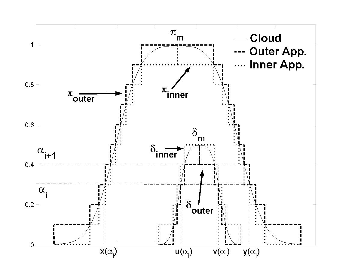
Figure 7. Inner and outer approximations of a non-comonotonic clouds

Given the above transformations, ${\mathcal{P}}(\underline{\pi}_{n})\subset{\mathcal{P}}(\pi)\subset{\mathcal{P}}(\overline{\pi}_{n})$, and $\lim_{n\to\infty}{\mathcal{P}}(\underline{\pi}_{n})={\mathcal{P}}(\pi)$ and also $\lim_{n\to\infty}{\mathcal{P}}(\overline{\pi}_{n})={\mathcal{P}}(\pi)$. Similarly, ${\mathcal{P}}(1-\underline{\delta}_{n})\subset{\mathcal{P}}(1-\delta)\subset{\mathcal{P}}(1-\overline{\delta}_{n})$, $\lim_{n\to\infty}{\mathcal{P}}(1-\overline{\delta}_{n})={\mathcal{P}}(1-\delta)$ and $\lim_{n\to\infty}{\mathcal{P}}(1-\underline{\delta}_{n})={\mathcal{P}}(1-\delta)$. Since the set of probabilities induced by the cloud $[\delta,\pi]$ is ${\mathcal{P}}(\pi)\cap{\mathcal{P}}(1-\delta)$, it is clear that the two credal sets ${\mathcal{P}}(\underline{\pi}_{n})\cap{\mathcal{P}}(1-\underline{\delta}_{n})$ and ${\mathcal{P}}(\overline{\pi}_{n})\cap{\mathcal{P}}(1-\overline{\delta}_{n})$, are respectively inner and outer approximations of ${\mathcal{P}}(\pi)\cap{\mathcal{P}}(1-\delta)$. Moreover:

$$\lim_{n\to\infty}{\mathcal{P}}(\underline{\pi}_{n})\cap{\mathcal{P}}(1-\underline{\delta}_{n})={\mathcal{P}}(\pi)\cap{\mathcal{P}}(1-\delta)$$

$$\lim_{n\to\infty}{\mathcal{P}}(\overline{\pi}_{n})\cap{\mathcal{P}}(1-\overline{\delta}_{n})={\mathcal{P}}(\pi)\cap{\mathcal{P}}(1-\delta).$$

The random sets that are inner approximations (by proposition 5) of the finite clouds $[\underline{\delta}_{n},\underline{\pi}_{n}]$ and $[\underline{\delta}_{n},\underline{\pi}_{n}]$ converge to the continuous random set defined by the Lebesgue measure on the unit interval $\alpha\in[0,1]$ and the multimapping $\alpha\longrightarrow E_{\alpha}$ such that

$$E_{\alpha}=\{r\in\mathbb{R}|(\pi(r)\geq\alpha)\wedge(\delta(r)<\alpha)\}.$$

In the limit, it follows that this continuous random set is an inner approximation of the continuous cloud. ∎

References

• [1] D. A. Alvarez, On the calculation of the bounds of probability of events using infinite random sets, I. J. of Approximate Reasoning 43 (2006) 241–267.
• [2] A. Chateauneuf, Combination of compatible belief functions and relation of specificity, in: Advances in the Dempster-Shafer theory of evidence, John Wiley & Sons, Inc, New York, NY, USA, 1994, pp. 97–114.
• [3] A. Chateauneuf, J.-Y. Jaffray, Some characterizations of lower probabilities and other monotone capacities through the use of M bius inversion, Mathematical Social Sciences 17 (3) (1989) 263–283.
• [4] I. Couso, S. Montes, P. Gil, The necessity of the strong alpha-cuts of a fuzzy set, Int. J. on Uncertainty, Fuzziness and Knowledge-Based Systems 9 (2001) 249–262.
• [5] L. de Campos, J. Huete, S. Moral, Probability intervals: a tool for uncertain reasoning, I. J. of Uncertainty, Fuzziness and Knowledge-Based Systems 2 (1994) 167–196.
• [6] G. de Cooman, M. Troffaes, E. Miranda, n-monotone lower previsions and lower integrals, in: F. Cozman, R. Nau, T. Seidenfeld (eds.), Proc. 4th International Symposium on Imprecise Probabilities and Their Applications, 2005.
• [7] S. Destercke, D. Dubois, E. Chojnacki, Unifying practical representations of uncertainty. Part I: Generalized p-boxes, Submitted to Int. J. of Approximate Reasoning.
• [8] D. Dubois, L. Foulloy, G. Mauris, H. Prade, Probability-possibility transformations, triangular fuzzy sets, and probabilistic inequalities, Reliable Computing 10 (2004) 273–297.
• [9] D. Dubois, H. Nguyen, H. Prade, Possibility theory, probability and fuzzy sets: misunderstandings, bridges and gaps, in: D. Dubois, H. Prade (eds.), Fundamentals of Fuzzy Sets, Kluwer, 2000, pp. 343–438.
• [10] D. Dubois, H. Prade, Fuzzy Sets and Systems: Theory and Applications, Academic Press, New York, 1980.
• [11] D. Dubois, H. Prade, Aggregation of possibility measures, in: J. Kacprzyk, M. Fedrizzi (eds.), Multiperson Decision Making using Fuzzy Sets and Possibility Theory, Kluwer, Dordrecht, the Netherlands, 1990, pp. 55–63.
• [12] D. Dubois, H. Prade, Interval-valued fuzzy sets, possibility theory and imprecise probability, in: Proceedings of International Conference in Fuzzy Logic and Technology (EUSFLAT’05), Barcelona, 2005.
• [13] D. Dubois, H. Prade, S. Sandri, On possibility/probability transformations, in: Proc. of the Fourth International Fuzzy Systems Association World Congress (IFSA’91), Brussels, Belgium, 1991.
• [14] S. Ferson, L. Ginzburg, V. Kreinovich, D. Myers, K. Sentz, Constructing probability boxes and Dempster-Shafer structures, Tech. rep., Sandia National Laboratories (2003).
• [15] M. Fuchs, A. Neumaier, Potential based clouds in robust design optimization, Journal of statistical theory and practice To appear.
• [16] M. Masson, T. Denoeux, Inferring a possibility distribution from empirical data, Fuzzy Sets and Systems 157 (3) (2006) 319–340.
• [17] A. Neumaier, Clouds, fuzzy sets and probability intervals, Reliable Computing 10 (2004) 249–272.
• [18] A. Neumaier, On the structure of clouds, Available on http://www.mat.univie.ac.at/$\sim$neum (2004).
• [19] P. Smets, Belief functions on real numbers, I. J. of Approximate Reasoning 40 (2005) 181–223.
• [20] P. Walley, Statistical reasoning with imprecise Probabilities, Chapman and Hall, New York, 1991.
• [21] L. Zadeh, The concept of a linguistic variable and its application to approximate reasoning- Part I, Information Sciences 8 (1975) 199–249.
• [22] L. Zadeh, Fuzzy sets as a basis for a theory of possibility, Fuzzy Sets and Systems 1 (1978) 3–28.