KUNS-2153

Fuzzy Ring from M2-brane Giant Torus

Tatsuma Nishioka and Tadashi Takayanagi

Department of Physics, Kyoto University, Kyoto 606-8502, Japan

We construct spinning dual M2 giant gravitons in $AdS_{4}\times S^{7}$, which generically become $\frac{1}{16}$ BPS states, and show that their world-volumes become torii. By taking an orbifold, we obtain spinning dielectric D2-brane configurations in $AdS_{4}\times CP^{3}$ dual to specific BPS operators in ABJM theory. This reveals a novel mechanism how to give an angular momentum to a dielectric D2-brane. We also find that when its angular momentum in the $AdS_{4}$ becomes large, it approaches to a ring-like object. Our result might suggest an existence of supersymmetric black rings in the $AdS_{4}$ background. We will also discuss dual giant gravitons in $AdS_{4}\times CP^{3}$.

1 Introduction

The studies of D-branes and M-branes have certainly been crucial in recent developments of string theory and M-theory. The classical dynamics of a brane is described by its world-volume theory, which is reparametrization invariant. At the same time, they are the sources of various gauge fields such as RR-fields. Thus the dynamics of their world-volumes is largely affected by the presence of the various fluxes in string theory and M-theory.

In particular, consider a D2-D0 bound state in type IIA string with the RR-3 form flux in the world-volume direction. Then it is well-known that the stable world-volume is given by a two sphere, called the fuzzy sphere (or dielectric D2-brane) [1]. This configuration can be regarded as a system of multiple D0-branes, which are expanded into a sphere due to the non-abelian RR coupling [1]. In the beginning of this paper, we will explicitly construct a supersymmetric fuzzy sphere in the fully back-reacted IIA background of $AdS_{4}\times CP^{3}$ [2, 3]. This predicts a new class of supersymmetric states in the dual ABJM theory [3].

We may naturally think a fuzzy sphere as a rigid body in the low energy limit since it is composed of infinitesimally small and massive constituents (i.e. D0-branes). This suggests, for example, that we can give it an angular momentum. Actually, by colliding closed strings with the fuzzy sphere, we can excite the angular momentum. However, naively this contradicts with the D2-brane description because the world-volume theory is reparametrization invariant and there seems no room for adding any angular momenta.

One of the main purposes of this paper is to resolve this puzzle completely. We argue that the spinning fuzzy ‘sphere’ is realized by putting a non-vanishing electric flux so that it produces the non-zero Poynting vector together with the magnetic flux due to the D0-brane charge (see Fig.1). Even though this is similar to the mechanism of the supertube [4], our case is far more non-trivial since the Gauss law on the sphere seems to contradict the presence of the electric flux. Indeed, as we will show explicitly, the topology of the world-volume is no longer a sphere but it should be changed into a torus in order to realize a stationary spinning configuration. This topology change is naturally explained by interpreting the sources of electric flux as the fundamental strings attached on the North and South Poles of the two sphere as explained in Fig.1. When its angular momentum in the $AdS_{4}$ becomes large, the fuzzy torus degenerates into a ring-like object (‘fuzzy ring’). Since some of such fuzzy rings become BPS states, they may resemble supersymmetric black rings [5].

Another D-brane configuration, which is analogous to the previous example, will be the giant gravitons [6, 7, 8, 9]. Here we especially consider dual giant gravitons in $AdS_{4}\times S^{7}$. It is a spherical M2-brane with angular momenta (or R-charges in the dual $CFT_{3}$) in the $S^{7}$ direction. As we will show in this paper, its reduction to the type IIA string via the orbifolding procedure introduced in [3], precisely leads to the mentioned spherical dielectric D2-brane in $AdS_{4}\times CP^{3}$.

Moreover, we will construct a spinning dual giant gravitons in M-theory by solving the BPS equations explicitly. By reducing them to type IIA via the orbifold, we will obtain the exact solution of the spinning fuzzy D2-brane. We will show that the world-volumes of a spinning giant graviton becomes a sphere (see Fig.2) with two spikes attached or a torus (see Fig.3).

This paper is organized as follows: In section two, we briefly review the M-theory on $AdS_{4}\times S^{7}$ and type IIA string on $AdS_{4}\times CP^{3}$. In section three, we construct a dielectric D2-brane solution in $AdS_{4}\times CP^{3}$ and show that it can be obtained from the reduction of a dual giant graviton in $AdS_{4}\times S^{7}$ by the orbifolding. In section four, we construct spinning dual giant gravitons in $AdS_{4}\times S^{7}$ by solving the BPS equations. In section five, we obtain the spinning dielectric D2-brane solution in the $AdS_{4}\times CP^{3}$ by taking the orbifold reduction of the spinning giant graviton solutions. In section 6, we construct dual giant gravitons in type IIA string on $AdS_{4}\times CP^{3}$. In section 7, we summarize the conclusion.

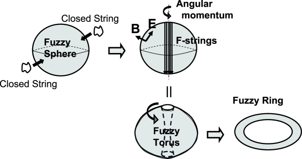
Figure 1: If we collides closed strings with a fuzzy sphere (or a dielectric D2-brane), it should begin spinning. To give a non-vanishing angular momentum, we need fundamental strings which connect between the North Pole and the South Pole. By regarding the total system as a bound state of a D2-brane, D0-branes and F-strings, its world-volume becomes a torus. In this paper we will present an exact profile of this configuration by solving the BPS equation.

2 Review of M-theory on $AdS_{4}\times S^{7}/Z_{k}$ and IIA on $AdS_{4}\times CP^{3}$

The near horizon metric of $N^{\prime}(=Nk)$ M2-branes becomes $AdS_{4}\times S^{7}$

$$ds^{2} =\frac{R^{2}}{4}\left[ds^{2}_{AdS_{4}}+4d\Omega_{7}^{2}\right],\qquad R=l_{p}(2^{5}\pi^{2}N^{\prime})^{\frac{1}{6}},$$ (2.1)

$$ds^{2}_{AdS_{4}} =-\left(1+r^{2}\right)dt^{2}+\frac{dr^{2}}{1+r^{2}}+r^{2}(d{\theta}^{2}+\sin^{2}\theta d\varphi^{2}),$$

with 4-form flux

$$F^{(4)}=-\frac{3R^{3}}{8}r^{2}\sin{\theta}dt\wedge dr\wedge d{\theta}\wedge d\varphi,$$ (2.2)

where $\Omega_{7}$ represents the coordinate of $S^{7}$ with unit radius:

$$|z_{1}|^{2}+|z_{2}|^{2}+|z_{3}|^{2}+|z_{4}|^{2}=1.$$ (2.3)

We can express

$$z_{i}=\mu_{i}e^{i\xi_{i}},\ \ \ \ (i=1,2,3,4)$$ (2.4)

where $(\mu_{1},\mu_{2},\mu_{3},\mu_{4})=(\sin\alpha,\cos\alpha\sin\beta,\cos\alpha\cos\beta\sin\gamma,\cos\alpha\cos\beta\cos\gamma)$. We choose the coordinate $(x^{0},x^{1},...,x^{10})$ as follows

$$x^{0}=t,\ \ x^{1}=r,\ \ x^{2}=\theta,\ \ x^{3}=\varphi,\ \ x^{4}=\alpha,\ \$$

$$x^{5}=\beta,\ \ x^{6}=\gamma,\ \ x^{7}=\xi_{1},\ \ x^{8}=\xi_{2},\ x^{9}=\xi_{3},\ \ x^{10}=\xi_{4}.$$ (2.5)

Our convention of $\Gamma$ matrices is such that $\gamma^{\mu}$ are normalized such that $\{\gamma_{\mu},\gamma_{\nu}\}=2\eta_{\mu\nu}$; on the other hand, $\Gamma^{\mu}$ are not normalized i.e. $\{\Gamma_{\mu},\Gamma_{\nu}\}=2g_{\mu\nu}$. Then the Killing spinors ${\epsilon}$ on $AdS_{4}\times S^{7}$ are found to be (see appendix A)

$${\epsilon}=e^{\frac{\alpha}{2}\hat{\gamma}\gamma_{4}}e^{\frac{\beta}{2}\hat{\gamma}\gamma_{5}}e^{\frac{\gamma}{2}\hat{\gamma}\gamma_{6}}e^{\frac{\xi_{1}}{2}\gamma_{47}}e^{\frac{\xi_{2}}{2}\gamma_{58}}e^{\frac{\xi_{3}}{2}\gamma_{69}}e^{\frac{\xi_{4}}{2}\hat{\gamma}\gamma_{10}}e^{-\frac{\rho}{2}\gamma_{1}\hat{\gamma}}e^{-\frac{t}{2}\gamma_{0}\hat{\gamma}}e^{\frac{\theta}{2}\gamma_{12}}e^{\frac{\varphi}{2}\gamma_{23}}{\epsilon}_{0}\equiv{\cal M}{\epsilon}_{0},$$ (2.6)

where we defined $\hat{\gamma}\equiv\gamma^{0123}$ and $\sinh\rho=r$; ${\epsilon}_{0}$ is a constant 11D spinor which satisfies ${\gamma}_{012345678910}{\epsilon}_{0}={\epsilon}_{0}$. It is easy to check $\{\hat{\gamma},{\gamma}_{a}\}=0,(a=0,1,2,3)$. As we can choose a constant spinor ${\epsilon}_{0}$ arbitrary, there are 32 Killing spinors in $AdS_{4}\times S^{7}$ as is well-known.

Let us take the $Z_{k}$ orbifold of $S^{7}$ and reduce the M-theory background $AdS_{4}\times S^{7}/Z_{k}$ to the type IIA string background $AdS_{4}\times CP^{3}$ following [3]. The $Z_{k}$ quotient acts on the complex coordinates $z_{i}~{}(i=1,2,3,4)$ as

$$z_{i}\sim e^{i\frac{2\pi}{k}}z_{i},$$ (2.7)

thus $\xi_{i}$ is identified as $\xi_{i}\sim\xi_{i}+\frac{2\pi}{k}$ under the orbifold action. If we define $\gamma_{47}{\epsilon}_{0}=is_{1}{\epsilon}_{0}$, $\gamma_{58}{\epsilon}_{0}=is_{2}{\epsilon}_{0}$ and $\gamma_{69}{\epsilon}_{0}=is_{3}{\epsilon}_{0}$, the spinors which survive the $Z_{k}$ orbifold projection are the ones $(s_{1},s_{2},s_{3})=(+,+,-),(+,-,+),(-,+,+),(+,-,-),(-,+,-),(-,-,+)$. The ones with $(+,+,+)$ and $(-,-,-)$ are projected out. Therefore 24 out of 32 Killing spinors are survived in the $AdS_{4}\times S^{7}/Z_{k}$ with $k>2$ as claimed in [3].

To see the reduction of our M-theory background to the type IIA string explicitly, it is easier to parameterize $S^{7}$ as follows (see [20]) instead of (2.4)

$$z_{1} =\cos\zeta~{}\cos\frac{\theta_{1}}{2}~{}e^{i\frac{\chi_{1}+\varphi_{1}}{2}},\qquad z_{2}=\cos\zeta~{}\sin\frac{\theta_{1}}{2}~{}e^{i\frac{\chi_{1}-\varphi_{1}}{2}},$$

$$z_{3} =\sin\zeta~{}\cos\frac{\theta_{2}}{2}~{}e^{i\frac{\chi_{2}+\varphi_{2}}{2}},\qquad z_{4}=\sin\zeta~{}\sin\frac{\theta_{2}}{2}~{}e^{i\frac{\chi_{2}-\varphi_{2}}{2}},$$ (2.8)

where the angular valuables run the values $0\leq\zeta<\frac{\pi}{2}$, $0\leq\chi_{i}<4\pi$, $0\leq\varphi_{i}\leq 2\pi$ and $0\leq\theta_{i}<\pi$.

Define new coordinates

$$\chi_{1}=2y+\psi,\ \ \ \ \ \ \ \chi_{2}=2y-\psi.$$ (2.9)

The $Z_{k}$ orbifold action is now given by $y\sim y+\frac{2\pi}{k}$. Then

$$ds_{S^{7}}^{2}=ds^{2}_{CP^{3}}+(dy+A)^{2},$$ (2.10)

where $A$ is one form such that $dA=2J$ ($J$ is the Kahler form of $CP^{3}$). By comparing the above result with the conventional reduction formula, we obtain type IIA background $AdS_{4}\times CP^{3}$ with 1-form and 3-form RR potentials as follows (setting $\alpha^{\prime}=1$) [3, 2].

$$ds^{2} ={\tilde{R}}^{2}(ds_{AdS_{4}}^{2}+4ds_{CP^{3}}^{2}),$$

$$ds_{CP^{3}}^{2} =d\zeta^{2}+\cos\zeta^{2}\sin^{2}\zeta\left(d\psi+\frac{\cos\theta_{1}}{2}d\varphi_{1}-\frac{\cos\theta_{2}}{2}d\varphi_{2}\right)^{2}$$

$$\quad+\frac{1}{4}\cos^{2}\zeta\left(d\theta_{1}^{2}+\sin^{2}\theta_{1}d\varphi_{1}^{2}\right)+\frac{1}{4}\sin^{2}\zeta(d\theta_{2}^{2}+\sin^{2}\theta_{2}d\varphi_{2}^{2}),$$ (2.11)

$$C^{(1)} =\frac{k}{2}\left[(\cos^{2}\zeta-\sin^{2}\zeta)d\psi+\cos^{2}\zeta\cos\theta_{1}d\varphi_{1}+\sin^{2}\zeta\cos\theta_{2}d\varphi_{2}\right],$$

$$C^{(3)} =-\frac{k{\tilde{R}}^{2}}{2}r^{3}\sin{\theta}dt\wedge d{\theta}\wedge d\varphi,$$

$$e^{2\phi} =\frac{4{\tilde{R}}^{2}}{k^{2}},\qquad{\tilde{R}}^{2}=\frac{R^{3}}{4k}=\pi\sqrt{\frac{2N}{k}}.$$

Again, this background preserves 24 supersymmetries and its holographic dual is recently argued to be the three dimensional ${\cal N}=6$ Chern-Simons theory (ABJM theory) [3].

3 Fuzzy Sphere and Dual Giant Gravitons

3.1 Dual Giant Gravitons in M-theory

Consider a dual giant graviton expanding spherically in $AdS_{4}$ and rotating in the $y$ direction of $S^{7}$ given in (2.10). We take the world-volume coordinates of the M2-brane as

$$\sigma_{0}\equiv\tau=t,\quad\sigma_{1}={\theta},\quad\sigma_{2}=\varphi,$$ (3.1)

and assume the transverse coordinates except $y$ does not depend on the world-volume coordinates, and $y$ depends on $t$ as

$$y=y(t).$$ (3.2)

Remember that this coordinate $y$, defined in (2.10), is the diagonal part of $\xi_{i}\ \ (i=1,2,3,4)$ in (2.4) and we fix both the non-diagonal part of $\xi_{i}$ and the values of $(\alpha,\beta,\gamma)$ to be constant. The action for this ansatz is given by the DBI action and the Chern-Simons term

$$S =-T_{2}\int d^{3}\sigma\sqrt{-\det(P[G]_{ij})}-T_{2}\int P[C^{(3)}],$$

$$=-\frac{\pi R^{3}T_{2}}{2}\int dt\left[r^{2}\sqrt{1+r^{2}-4{\dot{y}}^{2}}-r^{3}\right],$$ (3.3)

where $i,j$ and $P[\dots]$ denote the world-volume coordinates and the pull-back on the world-volume respectively. The tension is given by $T_{2}=\frac{1}{(2\pi)^{2}}$ in our convention. The conserved momentum conjugate to $y$ becomes

$$P_{y}=2\pi R^{3}T_{2}\frac{r^{2}\dot{y}}{\sqrt{1+r^{2}-4{\dot{y}}^{2}}},$$ (3.4)

and the Hamiltonian becomes using $P_{y}$

$$H =P_{y}\dot{y}-L$$

$$=\frac{\pi R^{3}T_{2}}{2}\left[\sqrt{1+r^{2}}\sqrt{r^{4}+\frac{P_{y}^{2}}{(\pi R^{3}T_{2})^{2}}}-r^{3}\right].$$ (3.5)

Thus we obtain the solution satisfying $\partial H/\partial r=0$ as

$$r=0,\qquad\sqrt{\frac{P_{y}^{2}}{(\pi R^{3}T_{2})^{2}}}.$$ (3.6)

The former is a graviton and the latter is a giant graviton solution. Substituting these into (3.4), we can determine the dependence on $t$ of $y$ as $y=\frac{t}{2}$ or equally,

$$\xi_{1}=\xi_{2}=\xi_{3}=\xi_{4}=\frac{t}{2}.$$ (3.7)

Then the graviton and giant graviton rotate with the velocity of light and have equal energies

$$E=\frac{P_{y}}{2}=\frac{1}{2}(J_{1}+J_{2}+J_{3}+J_{4}),$$ (3.8)

where $J_{i}=P_{\xi_{i}}$ are the momenta in the $\xi_{i}$ direction.

For example, if only one of $J_{i}$ is non-vanishing, this relation (3.8) shows the giant graviton is $\frac{1}{2}$ BPS state [7] (for the properties of the supersymmetric states in the dual $CFT_{3}$ see e.g.[21]). In the same way we can have $1/4$ and $1/8$ BPS dual giants depending on the values of $(\alpha,\beta,\gamma)$ as we will show in section 4. The result is summarized in Table.1.

3.2 Fuzzy Sphere in $AdS_{4}$

Now we would like to show that dielectric D2-branes [1] (or fuzzy spheres) can be realized in the $AdS_{4}\times CP^{3}$ background (2). It expands spherically in $AdS_{4}$ and we take the world-volume coordinates of D2-brane as

$$\sigma_{0}\equiv\tau=t,\sigma_{1}={\theta},\sigma_{2}=\varphi,$$ (3.9)

and introduce the $U(1)$ field strength, describing the $M$ D0-brane charge

$$F=\frac{M}{2}\sin{\theta}d{\theta}\wedge d\varphi.$$ (3.10)

Assuming the solution does not depend on $t$, the action for D2-brane becomes

$$S= =-T_{2}\int d^{3}\sigma e^{-\phi}\sqrt{-\det(P[G]_{ij}+2\pi F_{ij})}-T_{2}\int P[C^{(3)}]$$

$$=-2\pi T_{2}\,kR^{2}\int dt\left[\sqrt{r^{2}+1}\sqrt{r^{4}+\frac{\pi^{2}M^{2}}{R^{4}}}-r^{3}\right].$$ (3.11)

Since this Lagrangian consists of only potential term, the solution is easily obtained by minimizing the Hamiltonian $H$ leading to

$$r=\frac{\pi M}{R^{2}},\qquad H=2\pi^{2}T_{2}\,kM.$$ (3.12)

In our convention we have $T_{2}=\frac{1}{(2\pi)^{2}}$ and thus we find the energy of the fuzzy sphere

$$E=\frac{kM}{2},\ \ \ \ \left(r=M\sqrt{\frac{k}{2N}}~{}\right).$$ (3.13)

The above fuzzy sphere configurations composed of the D2-D0 bound states descend from the dual giant M2-branes in $AdS_{4}\times S^{7}/Z_{k}$, which is rotating in the $\partial_{y}$ direction. This is easily seen by taking the $Z_{k}$ orbifold $y\to y+\frac{2\pi}{k}$ of the dual giant in section 3.1. Indeed, the sum of the R-charges is quantized as $J_{1}+J_{2}+J_{3}+J_{4}\in kZ$ due to the orbifold projection, leading to the agreement between (3.13) and (3.8).

The fuzzy sphere D2-branes are parameterized by its position in $CP^{3}$ in the IIA description. Some of them preserve a half supersymmetries (12 SUSYs) when only one of $J_{i}\ \ (i=1,2,3,4)$ is non-zero as summarized in the $k>2$ case of the Table.1. Therefore, it is very interesting to consider its dual operator in the ABJM theory (for a recent study of operators in ABJM theory dual to giant gravitons refer to [22]) . When the number of D0-branes is $M$, the energy or conformal dimension is given by $E=\frac{kM}{2}$ and the baryon charge is $kM$. Thus it should be made of $k$ scalar fields of the matter fields $(A_{1},A_{2},\bar{B}_{1},\bar{B}_{2})$. In order to have a gauge invariant operator we need a contribution from the flux sector or the Wilson line in the sense of [3]. It will be an interesting future direction to pursuit the dual CFT operator in detail.

4 Spinning Dual Giant Gravitons in M-theory

As we have shown in the previous section the dual giant gravitons in M-theory on $AdS_{4}\times S^{7}/Z_{k}$ are equivalent to the dielectric D2-branes (fuzzy spheres) in type IIA string on $AdS_{4}\times CP^{3}$. Partly motivated by the problem raised in the introduction summarized in Fig.1, we would like to move on to a more non-trivial example by introducing a non-vanishing spin in the $AdS_{4}$ direction. Another motivation for this is to understand the $\frac{1}{16}$ BPS states in $AdS_{4}\times S^{7}$. In this section we will analyze the M-theory description of the spinning dual giant gravitons and construct exact solutions by solving the BPS equation. In the next section we reduce the solution to the fuzzy torus in type IIA string.

4.1 Spinning Giant Graviton Ansatz

We assume the following ansatz of the spinning dual giant graviton in $AdS_{4}\times S^{7}/Z_{k}$

$$r=r(\theta),\ \ \ \ y=w\varphi+\omega t,$$ (4.1)

where $w\in\frac{Z}{k}$ is the winding number equivalent to fundamental string charge (remember that $y$ is compactified as $y\sim y+\frac{2\pi}{k}$), while non-zero constant $\omega$ leads to the D$0$-brane charge after the Kaluza-Klein reduction.

Then the M$2$-brane world-volume theory becomes

$$S=-T_{2}\int dtd\theta d\varphi{\cal{L}},$$ (4.2)

where

$$\frac{8}{R^{3}}{\cal{L}}=\sqrt{\left(\frac{r^{\prime 2}}{1+r^{2}}+r^{2}\right)\left(r^{2}(1+r^{2})\sin^{2}\theta+4w^{2}(1+r^{2})-4\omega^{2}r^{2}\sin^{2}{\theta}\right)}-r^{3}\sin\theta.$$ (4.3)

4.2 Supersymmetry Condition (generic case)

We would like to find M2-brane configurations that preserve some supersymmetries. The projection operator of supersymmetries in the presence of M2-branes is given by

$$\Gamma=\frac{1}{3!\sqrt{-\det P[G]}}{\epsilon}^{ijk}\partial_{i}X^{\mu}\partial_{j}X^{\nu}\partial_{k}X^{\rho}\Gamma_{\mu\nu\rho},$$ (4.4)

which always satisfies $\Gamma^{2}=1$. We will analyze the supersymmetry conditions closely following the general strategy in [9], where non-spinning dual giants in $AdS_{5}\times S^{5}$ has been studied. In this subsection we assume that the M2-brane is situated at a generic point of $(\alpha,\beta,\gamma)$ in the coordinate system (2.5). In section 4.5, we will discuss the issue that the number of preserved supersymmetries is enhanced at particular values of $(\alpha,\beta,\gamma)$.

To examine the supersymmetry condition, let us notice $\Gamma_{y}=R\sum_{i=1}^{4}\mu_{i}\gamma_{6+i}$. Instead we will write $\Gamma_{y}=R\gamma_{y}$ for simplicity, but notice that $\gamma_{y}$ depends on the coordinate $\alpha,\beta$ and $\gamma$. In the end we find (we define $r\equiv\sinh\rho$)

$$\Gamma =\frac{1}{3!\sqrt{-\det P[G]}}(\Gamma_{0}+\omega\Gamma_{y})(\Gamma_{2}+r^{\prime}\Gamma_{1})(\Gamma_{3}+w\Gamma_{y})+(\mbox{perm})$$

$$=\frac{R^{3}}{8\cdot 3!\sqrt{-\det P[G]}}\left(\sqrt{1+r^{2}}\ \gamma_{0}+2\omega\gamma_{y}\right)\left(r\gamma_{2}+\frac{r^{\prime}}{\sqrt{1+r^{2}}}\gamma_{1}\right)(r\sin\theta\gamma_{3}+2w\gamma_{y})+(\mbox{perm})$$

$$=\frac{R^{3}}{8\cdot\sqrt{-\det P[G]}}\Biggl{[}\sqrt{1+r^{2}}r^{2}\sin\theta\gamma_{023}+2rw\sqrt{1+r^{2}}~{}\gamma_{02y}+r^{\prime}r\sin\theta~{}\gamma_{013}+2r^{\prime}w\gamma_{01y}$$

$$\qquad+2\omega r^{2}\sin\theta~{}\gamma_{y23}+\frac{2\omega r^{\prime}r\sin\theta}{\sqrt{1+r^{2}}}~{}\gamma_{y13}\Biggr{]}$$

$$=\frac{R^{3}}{8\cdot\sqrt{-\det P[g]}}(\rho^{\prime}{\gamma}_{1}+\sinh\rho{\gamma}_{2})\Biggl{[}2(\omega\sinh\rho\sin{\theta}{\gamma}_{3}-w\cosh\rho{\gamma}_{0}){\gamma}_{y}-\sinh\rho\cosh\rho\sin{\theta}{\gamma}_{03}\Biggr{]},$$ (4.5)

and

$$\sqrt{-\det P[G]}=\frac{R^{3}}{8}\sqrt{(\rho^{\prime 2}+\sinh^{2}\rho)(\sinh^{2}\rho\cosh^{2}\rho\sin^{2}{\theta}+4w^{2}\cosh^{2}\rho-4\omega^{2}\sinh^{2}\rho\sin^{2}{\theta})}.$$ (4.6)

The M2-brane preserves a fraction of supersymmetries specified by

$$(\Gamma+1){\epsilon}=0,$$ (4.7)

out of the total 24 (or 32) Killing spinors when $k=1,2$ (or when $k>2$). This requirement is highly non-trivial since both $\Gamma$ and ${\epsilon}$ depend on the coordinates. Multiplying $(\rho^{\prime}{\gamma}_{1}+\sinh\rho{\gamma}_{2})$ from the left, (4.7) becomes

$$\left[\sqrt{s}\big{\{}\sinh\rho\sin{\theta}{\gamma}_{3}(2\omega{\gamma}_{y}+\cosh\rho{\gamma}_{0})-2w\cosh\rho{\gamma}_{0}{\gamma}_{y}\big{\}}+\rho^{\prime}{\gamma}_{1}+\sinh\rho{\gamma}_{2}\right]{\cal M}{\epsilon}_{0}=0,$$

$$\qquad\sqrt{s}\equiv\sqrt{\frac{\rho^{\prime 2}+\sinh^{2}\rho}{\sinh^{2}\rho\cosh^{2}\rho\sin^{2}{\theta}+4w^{2}\cosh^{2}\rho-4\omega^{2}\sinh^{2}\rho\sin^{2}{\theta}}}.$$ (4.8)

To find the configuration preserving the supersymmetry, we suppose the following conditions so that the above projection does not depend on ${\alpha},{\beta},{\gamma}$ when we move ${\cal M}$ to the left

$$({\gamma}_{47}-{\gamma}_{10}\hat{\gamma}){\epsilon}_{0}=0,\qquad({\gamma}_{58}-{\gamma}_{10}\hat{\gamma}){\epsilon}_{0}=0,$$

$$({\gamma}_{69}-{\gamma}_{10}\hat{\gamma}){\epsilon}_{0}=0.$$ (4.9)

These three conditions are not independent because of the relation ${\gamma}_{012345678910}{\epsilon}_{0}={\epsilon}_{0}$ and the two of them become independent. Under this conditions, we can move the matrix ${\cal M}$ to the left using the identities (B) given in the appendix

$${\cal M}\Bigg{[} e^{t{\gamma}_{0}\hat{\gamma}}\sinh\rho\Big{\{}\!\cosh\rho\sqrt{s}\big{\{}\!2w\cos{\theta}{\gamma}_{2310}+\sin{\theta}(\sin\varphi{\gamma}_{2}\!-\!\cos\varphi{\gamma}_{3}){\gamma}_{10}(2\omega\!-\!{\gamma}_{010}\!-\!2w{\gamma}_{1})\big{\}}\!-\!\rho^{\prime}\hat{\gamma}\Big{\}}$$

$$+\big{\{}(\rho^{\prime}\cosh\rho\cos{\theta}-\sinh\rho\sin{\theta}){\gamma}_{1}-2w\cosh^{2}\rho\sqrt{s}{\gamma}_{010}-2\omega\sinh^{2}\rho\sin^{2}{\theta}\sqrt{s}{\gamma}_{0110}\big{\}}$$

$$+(\cos\varphi{\gamma}_{2}+\sin\varphi{\gamma}_{3})\big{\{}\rho^{\prime}\cosh\rho\sin{\theta}+\sinh\rho\cos{\theta}-2\omega\sinh^{2}\rho\sin{\theta}\cos{\theta}\sqrt{s}{\gamma}_{010}\big{\}}\Bigg{]}{\epsilon}_{0}=0$$ (4.10)

To drop the time dependence in the first line, the following two conditions are needed

$$(2\omega-{\gamma}_{010}-2w{\gamma}_{1}){\epsilon}_{0}=0,$$

$${\gamma}_{023}\left(-2w\cosh\rho\cos{\theta}\sqrt{s}{\gamma}_{010}+\rho^{\prime}{\gamma}_{1}\right){\epsilon}_{0}=0.$$ (4.11)

Since ${\gamma}_{1}$ and ${\gamma}_{010}$ commute with each other, we can simultaneously diagonalize these matrices. Denoting the eigenvalues of these matrices by $\eta_{1}(=\pm 1)$ and $\eta_{2}(=\pm 1)$ respectively, the above equations are solved by

$$2\omega =\eta_{2}(2\eta_{1}\eta_{2}w+1),$$

$$\rho^{\prime} =-\frac{2\eta_{1}\eta_{2}w\sinh\rho\cosh\rho\cos{\theta}}{(\sinh^{2}\rho-2\eta_{1}\eta_{2}w)\sin{\theta}}\qquad(\eta_{1}\eta_{2}w>0,\quad\sinh^{2}\rho<2|w|)$$ (4.12)

$$=\frac{2\eta_{1}\eta_{2}w\sinh\rho\cosh\rho\cos{\theta}}{(\sinh^{2}\rho-2\eta_{1}\eta_{2}w)\sin{\theta}}\qquad(\mbox{otherwise})$$ (4.13)

Moreover, we can check whether the second and third line of (4.2) vanish or not, and we eventually find that only the latter case i.e. (4.13) satisfies it. The conditions (4.2) and (4.2) for the Killing spinor tell that this solution is (at least) $\frac{1}{16}$ BPS.

The solution (4.13) is classified into the following two types:

• For $\eta_{1}\eta_{2}w<0$, $\rho$ decreases monotonically from $\rho(0)=\infty$ to $\rho\left(\frac{\pi}{2}\right)$ with ${\theta}$ varying from $0$ to $\frac{\pi}{2}$.

• For $\eta_{1}\eta_{2}w>0$ and $\sinh^{2}\rho\geq 2|w|$, $\rho$ increases from $\rho({\theta}_{0})$ to $\rho(\frac{\pi}{2})$ with ${\theta}$ varying from ${\theta}_{0}$ to $\frac{\pi}{2}$, satisfying $\sinh^{2}\rho({\theta}_{0})=2\eta_{1}\eta_{2}w$.

We can extend these solutions beyond $\theta=\frac{\pi}{2}$ in a symmetric way under the $Z_{2}$ action $\theta\to\pi-\theta$. In the first case, we will have a sphere with two spikes attached (we will analyze this in detail later, see Fig.2). In the second case, the M2-brane world-volume naively ends at $\theta=\theta_{0}$. This is due to the assumption that $r$ is single-valued function of ${\theta}$ in deriving (4.7). Actually, the correct interpretation of the second case turns out to be a toroidal world-volume (as we will examine in detail later, see Fig.3), where $r$ becomes double-valued. That is to say, the above description covers only a half part of the whole configuration. If we choose the appropriate world-volume coordinate $\chi$ corresponding to the one cycle of the torus, instead of ${\theta}$, the relation between the $\kappa$-projection gamma matrices (4.4) becomes

$${\Gamma}(t,\chi,\varphi)=\frac{\partial{\theta}/\partial\chi}{|\partial{\theta}/\partial\chi|}{\Gamma}(t,{\theta},\varphi).$$ (4.14)

Therefore, in second case, the sign flips at ${\theta}={\theta}_{0}$ and we must use

$$(-{\Gamma}+1){\epsilon}=0$$ (4.15)

instead of (4.7) to extend the above configuration. We can solve this equation similarly and obtain the supersymmetric solution which connects the above solution as

$$\rho^{\prime} =\frac{2\eta_{1}\eta_{2}w\sinh\rho\cosh\rho\cos{\theta}}{(\sinh^{2}\rho-2\eta_{1}\eta_{2}w)\sin{\theta}}\qquad(\eta_{1}\eta_{2}w>0,\quad\sinh^{2}\rho\leq 2|w|).$$ (4.16)

In summary, we find that a spinning dual M2-giant in $AdS_{4}\times S^{7}$ (or $AdS_{4}\times S^{7}/Z_{2}$) becomes at least $\frac{1}{16}$ BPS state if the following BPS equation is satisfied

$$2\omega =\eta_{2}(2\eta_{1}\eta_{2}w+1),$$

$$\rho^{\prime} =\frac{2\eta_{1}\eta_{2}w\sinh\rho\cosh\rho\cos{\theta}}{(\sinh^{2}\rho-2\eta_{1}\eta_{2}w)\sin{\theta}}.$$ (4.17)

We can also rewrite this BPS equation in terms of the coordinate $r$

$$\frac{dr}{d\theta}=2\eta_{1}\eta_{2}w\frac{r(1+r^{2})}{r^{2}-2\eta_{1}\eta_{2}w}\cdot\frac{\cos\theta}{\sin\theta}.$$ (4.18)

As we will explain in the next subsection, it becomes $\frac{1}{4}$ or $\frac{1}{8}$ BPS states if we choose specific values of $\alpha,\beta$ and $\gamma$. We will leave the details of the analysis of supersymmetry enhancement to the section 4.5.

A spinning dual M2-giant in $AdS_{4}\times S^{7}/Z_{k}\ \ (k>2)$ can be treated similarly by just taking the orbifold $y\sim y+\frac{2\pi}{k}$. This orbifold projection kills some of the supersymmetries. In fact, in the generic case, no supersymmetries will be left after the orbifolding. However, as we will explain in section 4.5, for specific values of $\alpha,\beta$ and $\gamma$, there will be remaining supersymmetries, leading to $\frac{1}{4}$ or $\frac{1}{12}$ BPS states in $AdS_{4}\times S^{7}/Z_{k}$.

4.3 BPS Equation from Bogomolnyi Bound

In this section, we derive the supersymmetric equation (4.2) or (4.18) from another approach of the Bogomolnyi bound. We can show the DBI part of the action is rewritten as follows

$$\frac{8}{R^{3}}\sqrt{-P[G]}=\sqrt{\left(\frac{r^{\prime 2}}{1+r^{2}}+r^{2}\right)\left(r^{2}(1+r^{2})\sin^{2}\theta+4w^{2}(1+r^{2})-4\omega^{2}r^{2}\sin^{2}\theta\right)}$$

$$=\sqrt{\left(2w\frac{d(r\cos\theta)}{d\theta}+\eta r^{3}\sin\theta\right)^{2}+\frac{(r^{2}+2w)^{2}\sin^{2}\theta}{1+r^{2}}\left(\frac{dr}{d\theta}-\frac{2\eta wr(1+r^{2})\cos{\theta}}{(r^{2}-2\eta w)\sin{\theta}}\right)^{2}},$$ (4.19)

imposing the relation

$$\omega=\pm\left(w+\frac{\eta}{2}\right),$$ (4.20)

where we can allow both signs $\eta=\pm 1$, corresponding to the freedom $\eta_{1}\eta_{2}=\pm 1$ in (4.18). If the BPS equation (4.18) or equally

$$\frac{dr}{d\theta}=2\eta w\frac{r(1+r^{2})}{r^{2}-2\eta w}\cdot\frac{\cos\theta}{\sin\theta},$$ (4.21)

is satisfied (setting $\eta=\eta_{1}\eta_{2}$), then the total Lagrangian

$$\frac{8}{R^{3}}{\cal{L}}=\frac{8}{R^{3}}\sqrt{-P[G]}\pm r^{3}\sin\theta=\mp 2\eta w\frac{d(r\cos\theta)}{d\theta},$$ (4.22)

successfully becomes a total derivative as required from the ordinary Bogomolnyi bound argument. At the same time, this guarantees that the solution to the BPS equation (4.21) satisfied the equation of motion. Notice that the coefficient in front of $r^{3}\sin\theta$ represents whether we consider a M2-brane or an anti M2-brane. By plugging the explicit solutions, we can check that in the Lagrangian (4.22), the $r^{3}\sin\theta$ term from the square root always cancels out the $r^{3}\sin\theta$ term from the coupling to 3-form field. In this way, we rederived the BPS equation (4.2) or (4.18) from the Bogomolnyi bound argument.

We would also like to compute energy and angular momenta. There are five different angular momenta: $J_{i}=P_{\xi_{i}}\ \ (i=1,2,3,4)$ and $S=P_{\varphi}$. In the $AdS_{4}/CFT_{3}$ viewpoint $J_{i}$ is the R-charge and $S$ is the spin inside the $AdS_{4}$. They are obtained by taking the functional derivative as $P_{\varphi}=-T_{2}\int d\theta d\varphi\frac{\partial{\cal{L}}}{\partial\dot{\varphi}}$ and we find the linear relation

$$J_{i}=\frac{\mu_{i}^{2}}{w}S,$$ (4.23)

where $\mu_{i}=(\sin\alpha,\cos\alpha\sin\beta,\cos\alpha\cos\beta\sin\gamma,\cos\alpha\cos\beta\cos\gamma)$. If we define $J=\sum_{i=1}^{4}J_{i}~{}(=P_{y})$, then we find the relation $wJ=S$.

The energy is given by

$$E=\int d\theta d\varphi\left[\sum_{i=1}^{4}P_{\xi_{i}}\dot{\xi_{i}}-(-T_{2}){\cal L}\right]=\frac{\eta_{1}}{2}(2S+J_{1}+J_{2}+J_{3}+J_{4})+T_{2}\int d\theta d\varphi{\cal L},$$ (4.24)

where $\eta=\pm 1$ is the sign introduced in (4.13). Notice that this relation almost saturates the BPS bound expected from the dual $CFT_{3}$ since the final term $\int d\theta d\varphi{\cal L}$ is a total derivative (4.22).

4.4 Analytical Solutions to BPS Equation

Now let us solve the BPS equation (4.21) and determine the shape of M2-brane. We can analytically solve the differential equation and finally we get

$$\sin\theta=A\cdot r^{-1}(1+r^{2})^{\frac{1}{2}+\frac{1}{4\eta w}},$$ (4.25)

where $A$ is a constant. If we instead employ the coordinate $\rho$ we obtain

$$\sin\theta=A\cdot\frac{(\cosh\rho)^{1+\frac{1}{2\eta w}}}{\sinh\rho}.$$ (4.26)

Since the solution is $Z_{2}$ symmetric $r(\theta)=r(\pi-\theta)$, we have only to discuss the behavior of the function $r(\theta)$ for $0\leq\theta\leq\frac{\pi}{2}$. It is easy to see that when $\eta w<0$ there are only one value of $r$ which satisfies (4.25), while when $\eta w>0$ there are two such solutions. Accordingly, we have two different types of the M2-brane shape depending on the sign of $\eta w$.

4.4.1 Case 1: $\eta w<0$ (Giant Spike)

In this case, $r(\theta)$ is monotonically decreasing function when $0\leq\theta\leq\frac{\pi}{2}$. It satisfies $r(0)=\infty$ and $r(\frac{\pi}{2})=r_{0}$, where the constant $r_{0}>0$ is related to the integration constant $A$ via $A=r_{0}(1+r_{0}^{2})^{-\frac{1}{2}+\frac{1}{4|w|}}$. The shape of this M2-brane world-volume is plotted in Fig.2. It looks like a sphere with two spikes attached. The spikes are actually a cylinder with radius $\frac{R}{k}$ winding $wk$ times in the $y$ direction. Thus it can be regarded as a bound state of a (non-spinning) dual M2 giant and $wk$ tubular M2 branes.

Its energy is calculated from (4.24) as follows (we choose $\eta_{1}=+1$)

$$E-S-\frac{1}{2}(J_{1}+J_{2}+J_{3}+J_{4}) =\frac{R^{3}}{8}T_{2}\int d\theta d\varphi~{}2w[r\cos\theta]^{\prime}$$

$$=\pi wR^{3}T_{2}(r_{\infty}-r_{0}),$$ (4.27)

where $r_{\infty}$ presents the infinitely large value of $r$ at $\theta=0$ and $\theta=\pi$. Indeed the infinitely large contribution of right-hand side precisely coincides with the infinitely large mass of $kw$ M2-branes which wrap on the circle $\partial_{y}$ and which extend in the $r$ direction. We can explicitly express $J=\sum_{i=1}^{4}J_{i}$ as follows

$$J =\frac{R^{3}}{2}\omega T_{2}\int d\theta d\varphi r^{2}\sin^{2}\theta\sqrt{\frac{\frac{r^{\prime 2}}{1+r^{2}}+r^{2}}{r^{2}\sin^{2}\theta(1+r^{2})-4\omega^{2}r^{2}\sin^{2}\theta+4w^{2}(1+r^{2})}}$$

$$=2\pi R^{3}\omega T_{2}\int_{r_{0}}^{\infty}dr\frac{r^{2}\sin^{2}\theta}{2w(1+r^{2})\cos\theta}.$$ (4.28)

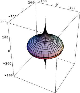
Figure 2: The giant-spike solution described in the three dimensional space $(r,\theta,\varphi)$ (we assumed $|w|=10$ and $A=3$). This corresponds to the sign $\eta w<0$. We multiplied the factor 10 with the horizontal coordinates.

4.4.2 Case 2: $\eta w>0$ (Giant Torus)

In this case, the values of $r$ in (4.25) is restricted to a certain range $r_{-}\leq r\leq r_{+}$ because the function $B(r)=r^{-1}(1+r^{2})^{\frac{1}{2}+\frac{1}{4|w|}}$ takes its minimum at $r=\sqrt{2w}$ and satisfies $B(0)=B(\infty)=\infty$. The values of $r_{\pm}$ are given by the two solutions to $Ar_{0}^{-1}(1+r_{0}^{2})^{\frac{1}{2}+\frac{1}{4|w|}}=1$. It is clear that we need to require $A<1/B(\sqrt{2w})$ in order to have any solution.

The values of $\theta$ is restricted to the range $\theta_{0}\leq\theta\leq\pi-\theta_{0}$ such that $r(\theta_{0})=\sqrt{2w}$. For a given $\theta$ there are two values of $r$ which satisfy (4.25). Thus we can conclude that the world-volume of this M2-brane is topologically a torus. An explicit shape of this M2-brane world-volume is plotted in Fig.3.

In this case, the total derivative term in (4.24) just vanishes since the world-volume has no boundary. Thus we obtain the standard BPS formula (choosing $\eta_{1}=+1$)

$$E=S+\frac{1}{2}(J_{1}+J_{2}+J_{3}+J_{4})=\omega J,$$ (4.29)

and

$$J=2\pi R^{3}\omega T_{2}\int_{r_{-}}^{r_{+}}dr\frac{r^{2}\sin^{2}\theta}{2w(1+r^{2})\cos\theta}.$$ (4.30)

It is interesting to note that if we fix $J$ and take $w$ to be large, then we can realize a ring-like object.

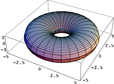
Figure 3: The giant-torus solution corresponding to the sign $\eta w>0$ (we assumed $|w|=10$ and $A=0.8$).

4.5 Enhanced Supersymmetries

In the previous subsection, we showed that the solution which satisfies (4.18) preserves at least two (i.e. $\frac{1}{16}$ BPS) of the total thirty-two supersymmetries in $AdS_{4}\times S^{7}$. Though for general values of ${\alpha},{\beta}$ and ${\gamma}$, the spinning dual giant is a $\frac{1}{16}$ BPS state, we can see that it enhances to $\frac{1}{4}$ or $\frac{1}{8}$ BPS states for specific values of ${\alpha},{\beta}$ and ${\gamma}$. In this subsection we will examine these details of supersymmetries in both $AdS_{4}\times S^{7}$ and its orbifold $AdS_{4}\times S^{7}/Z_{k}$. The result is summarized in the Table.1 (non-spinning case) and Table.2 (spinning case).

It is convenient to define the $\pm 1$ eigenvalues $\eta_{1},\eta_{2},s_{1},s_{2},s_{3}$ and $s_{4}$ of the commuting matrices $\gamma_{1},\gamma_{01\!0},\gamma_{47},\gamma_{58},\gamma_{69}$ and $\hat{\gamma}\gamma_{10}$ for a given spinor ${\epsilon}_{0}$ as we have already did so in previous sections

$$(\gamma_{1}-\eta_{1}){\epsilon}_{0}=0,\qquad(\gamma_{01\!0}-\eta_{2}){\epsilon}_{0}=0,$$

$$({\gamma}_{47}-is_{1}){\epsilon}_{0}=0,\qquad(\gamma_{58}-is_{2}){\epsilon}_{0}=0,$$

$$({\gamma}_{69}-is_{3}){\epsilon}_{0}=0,\qquad(\hat{\gamma}\gamma_{10}-is_{4}){\epsilon}_{0}=0.$$ (4.31)

Since the 11D spinor ${\epsilon}_{0}$ is chiral, we impose $\gamma_{01234567891\!0}{\epsilon}_{0}={\epsilon}_{0}$. This leads to the relation $s_{1}s_{2}s_{3}s_{4}=1$.

4.5.1 Enhanced Supersymmetries in $AdS_{4}\times S^{7}\ (\mbox{or}\ S^{7}/Z_{2})$

For example, if we set ${\alpha}={\beta}={\gamma}=0$ (called case (a)), we do not need to require any of the constraints in (4.2) because $\gamma_{y}=\gamma_{10}$. Thus in this case, it becomes $\frac{1}{4}$ BPS because we only need to fix the signs of $\eta_{1}$ and $\eta_{2}$. In a similar way, when two out of ${\alpha},{\beta}$ and ${\gamma}$ are vanishing (called case (b)), we get a $\frac{1}{8}$ BPS state by requiring a further constraint $s_{1}=s_{4}$, $s_{2}=s_{4}$ or $s_{3}=s_{4}$. For other generic values (case (c)), it becomes $\frac{1}{16}$ BPS as we already mentioned.

Also notice that non-spinning case $w=0$ is special. In this case we do not need to specify the value of $\eta_{1}$ as is clear from (4.2). Thus the number of preserved supersymmetries becomes doubled as summarized in Table.1.

4.5.2 Enhanced Supersymmetries in $AdS_{4}\times S^{7}/Z_{k}\ \ (k>2)$

The $Z_{k}$ orbifold action on the spinor ${\epsilon}_{0}$ produces the phase factor

$${\epsilon}_{0}\ \to\ e^{\frac{\pi i}{k}(s_{1}+s_{2}+s_{3}+s_{4})}{\epsilon}_{0}.$$ (4.32)

Thus for the M-theory on $AdS_{4}\times S^{7}/Z_{k}$ with $k>2$ (or IIA string on $AdS_{4}\times CP^{3}$), there are 24 Killing spinors corresponding to the choice $(+,+,-,-)$ and its permutations, which satisfies the orbifold projection $\sum_{i=1}^{4}s_{i}\equiv 0\ (\text{mod}~{}2)$ as already mentioned.

The number of supersymmetries for spinning or non-spinning dual giants can be analyzed in the same way as in the previous $k=1,2$ case. It is again summarized in Table.1 and Table.2.

$k$	Total SUSY	Case (a)	Case (b)	Case (c)
$k=1,2$	32	16	8	4
$k>2$	24	12	4	0

Table 1: The number of supersymmetries of dual non-spinning giant gravitons in $AdS_{4}\times S^{7}/Z_{k}$. Its world-volume looks like a sphere as usual. The result of dielectric D2-branes (or fuzzy sphere) in type IIA string on $AdS_{4}\times CP^{3}$ corresponds to the $k>2$ case. The case (a) is defined by $\alpha=\beta=\gamma$. The case (b) is by $\alpha=\beta$, $\beta=\gamma$ or $\alpha=\gamma$. The case (c) is all the other possibilities.

$k$	Total SUSY	Case (a)	Case (b)	Case (c)
$k=1,2$	32	8	4	2
$k>2$	24	6	2	0

Table 2: The number of supersymmetries of dual spinning giant gravitons in $AdS_{4}\times S^{7}/Z_{k}$. Its world-volume looks like either a torus or sphere with two spikes. The result of spinning dielectric D2-branes (or fuzzy torus) in type IIA string on $AdS_{4}\times CP^{3}$ corresponds to the $k>2$ case. The cases (a), (b) and (c) are defined in the same way as in Table.1.

5 Fuzzy Rings in $AdS_{4}$

As we learned in section 3, we can reduce a spherical dual giant graviton of M2-brane to a fuzzy sphere of a dielectric D2-brane in $AdS_{4}\times CP^{3}$ by considering the orbifold $AdS_{4}\times S^{7}/Z_{k}$. Thus it is intriguing to apply the same procedure to the spinning dual giant.

By construction, it is rotating both in the $y$ and $\varphi$ direction. The angular momentum $J=P_{y}\equiv kM$ leads to $M$ units of the D0-brane charge after the reduction to IIA string, while the winding number $w$ corresponds to the $wk$ units of the F-string charge. Therefore, the spinning dual giant constructed in the previous section will be reduced to a bound state of a D2-brane, $M$ D0-branes and $wk$ F-strings. Since the F-strings and D0-branes generate the electric and magnetic flux, the system has a non-vanishing Poynting vector which produces non-vanishing angular momentum (or spin) in the $\varphi$ direction. Indeed its value is given by $S=P_{\varphi}=wkM$. Notice that the quantization of the angular momentum is a consequence of the charge quantization of the F-string and D0-brane. In this way, in order to obtain a non-vanishing spin, the F-string charge is necessary.

One may notice that there are two different ways of attaching the F-string to the fuzzy sphere: (i) F-strings which are attached at north and south poles on the sphere and stretch toward the infinity (ii) F-strings which connects between the two poles. Indeed, the BPS equation in section 4 precisely leads to corresponding two solutions: giant spike and giant torus.

The profile of this dielectric D2-brane is again given by (4.25). The values of gauge fluxes can be computed by rewriting the action of a D2-brane into that of a M2-brane [24, 25]

$$S_{DBI} =-T_{2}\int_{D2}d^{3}x\ e^{-\phi}\sqrt{-\det(P[G^{(IIA)}]_{ij}+2\pi F_{ij})}$$

$$=-T_{2}\int_{D2}d^{3}x\left[e^{-\phi}\sqrt{-\det(P[G^{(IIA)}]_{ij}+e^{2\phi}a_{i}a_{j})}+\pi{\epsilon}^{ijk}a_{i}F_{jk}\right]$$ (5.1)

$$=-T_{2}\int_{M2}d^{3}x\sqrt{-\det(P[G^{(M)}]_{ij}+e^{\frac{4}{3}\phi}\partial_{i}\tilde{y}\partial_{j}\tilde{y})},$$

where we defined $\partial_{i}\tilde{y}=a_{i}$ in the final expression. The integration over the D2-brane gauge field $A_{i}$ requires the auxiliary vector field $a_{i}$ to be a total derivative. Notice also that the metric in M-theory and the IIA string frame metric is related via $ds^{2}_{M}=e^{-\frac{2}{3}\phi}ds^{2}_{IIA}+e^{\frac{4}{3}\phi}(d\tilde{y}+C)^{2}$. We can check the equivalence of the first line and the second line by integrating out $a_{i}$ explicitly.

The relation between $F_{ij}$ and $\partial_{i}\tilde{y}$ is given by

$$e^{\frac{4}{3}\phi}\sqrt{-\det P[G^{(M)}]}\frac{\partial^{i}\tilde{y}}{\sqrt{1+e^{\frac{4}{3}\phi}\partial_{i}\tilde{y}\partial^{i}\tilde{y}}}=-\pi{\epsilon}^{ijk}F_{jk},$$ (5.3)

where the left-hand side should be computed by using the M-theory metric.

By plugging $\tilde{y}=ky=k(\omega t+w\phi)$ (4.1) to (5.3), we eventually obtain the electric and magnetic field on the spinning dielectric D2-brane as follows

$$F_{t\theta}=-w\sqrt{\frac{2N}{k}}\cdot\frac{r(1+r^{2})}{|r^{2}-2\eta w|\sin\theta},$$

$$F_{\theta\varphi}=\omega\sqrt{\frac{2N}{k}}\cdot\frac{r^{3}\sin\theta}{|r^{2}-2\eta w|}.$$ (5.4)

Note that if we set $w=0$ and $\omega=\frac{1}{2}$, then we correctly reproduce $F_{t\theta}=0$ and $F_{\theta\varphi}=\frac{M}{2}\sin\theta$ as discussed in section 3.2.

In the same way as the spinning dual giant, we have two different types of the world-volume i.e. a sphere with two spikes (see Fig.2) and a torus (see Fig.3). The former case with infinitely long spikes is naturally understood as a bound state of the D2 fuzzy sphere and infinitely long fundamental strings. Since it has an infinite energy, it is not appropriate for the candidate of ‘rotating fuzzy sphere’ raised in the introduction of this paper. Instead, the fuzzy torus configuration will be a correct candidate as explained in Fig.1.

The supersymmetry of these D2-D0-F1 bound states is the same as the analysis of spinning dual giants in $AdS_{4}\times S^{7}/Z_{k}$ with $k$ sufficiently large and is shown in Table.2.

Finally we would like to note that it is possible to make one of two cycles of the torus very small so that it looks like a ring assuming $w$ is very large. By considering its back-reacted geometry, this fuzzy ring solution might suggest an existence of supersymmetric or non-supersymmetric black ring solutions in a certain $AdS_{4}$ supergravity. However, the topological censorship in $AdS_{4}$ [26] tells us that the horizon topology should always be $S^{2}$ and not $T^{2}$. Therefore, it is probable that it becomes a small black ring instead of a macroscopic one, by taking into account higher derivative corrections (see also [27] for a discussion of (small) black rings in four dimension). It is also a very interesting future problem to repeat a similar analysis for $AdS_{5}\times S^{5}$ and see if we can realize a fuzzy ring. If such an object exists, it might suggest supersymmetric black ring-like objects in $AdS_{5}$. An evidence for non-supersymmetric black ring solutions in $AdS$ has been given recently in [29].

6 Dual Giant Gravitons in Type IIA String on $AdS_{4}\times CP^{3}$

Before we conclude this paper, we would like to mention spherical D2-branes wrapped on $S^{2}$ in $AdS_{4}$ and orbiting the $CP^{3}$ as they are other interesting BPS states dual to supersymmetric operators in the ABJM theory. They can be regarded as dual giant gravitons in type IIA string on $AdS_{4}\times CP^{3}$. They are also obtained from the reduction of spherical dual giants in $AdS_{4}\times S^{7}/Z_{k}$.

We take the world-volume coordinates of D2-brane as

$$\sigma_{0}\equiv\tau=t,\sigma_{1}={\theta},\sigma_{2}=\varphi,$$ (6.1)

and consider a trial solution of the form

$$\psi=\psi(\tau),\quad\phi_{1}=\phi_{1}(\tau),\quad\phi_{2}=\phi_{2}(\tau),\quad\zeta,{\theta}_{1},{\theta}_{2},r=const.$$ (6.2)

Then, the D2-brane action is written as

$$S=-2\pi T_{2}\,kR^{2}\int dt[r^{2}{\Delta}^{1/2}-r^{3}],$$ (6.3)

where ${\Delta}\equiv P[G]_{tt}$ is given by (in the coordinate (2))

$${\Delta} =1+r^{2}-4\cos^{2}\zeta\sin^{2}\zeta\left(\dot{\psi}+\frac{\cos{\theta}_{1}}{2}\dot{\varphi}_{1}-\frac{\cos{\theta}_{2}}{2}\dot{\varphi}_{2}\right)^{2}$$

$$\quad-\cos^{2}\zeta\sin^{2}{\theta}_{1}\dot{\varphi}_{1}^{2}-\sin^{2}\zeta\sin^{2}{\theta}_{2}\dot{\varphi}_{2}^{2}.$$ (6.4)

Solving the above Lagrangian, we can obtain the spherical D2-brane solution. For simplicity, we take $\zeta=\frac{\pi}{4},{\theta}_{1}={\theta}_{2}=0$ and $\dot{\varphi}_{1}=\dot{\varphi}_{2}=0$. In this case, the Lagrangian (6.3) becomes

$$L=-a\left[r^{2}\sqrt{1+r^{2}-\dot{\psi}^{2}}-r^{3}\right],$$ (6.5)

where we denote $a=2\pi T_{2}\,kR^{2}$. The momentum conjugate to $\psi$ is

$$P_{\psi}=\frac{ar^{2}\dot{\psi}}{\sqrt{1+r^{2}-\psi^{2}}}.$$ (6.6)

Using this, the Hamiltonian becomes

$$H=P_{\psi}\dot{\psi}-L=a\left[\sqrt{r^{2}+1}\sqrt{r^{4}+\frac{P_{\psi}^{2}}{a^{2}}}-r^{3}\right].$$ (6.7)

Thus the solution satisfying $\partial H/\partial r=0$ is

$$r=0,\qquad r^{2}=\frac{P_{\psi}^{2}}{a^{2}}.$$ (6.8)

The former is graviton and the latter is giant graviton solution. These have the equal energy $E=P_{\psi}=\frac{1}{2}(J_{1}+J_{2}-J_{3}-J_{4})$. Since they do not rotate in the $y$ direction, the dual operators will not have any baryon charge. Therefore they should be dual to be singlet operators of the bi-fundamental matter fields such as the symmetric polynomials of $(A_{i}B_{j})$ as in the case of $AdS_{5}\times S^{5}$ [30].

7 Conclusion

In this paper we presented an analytical description of spinning dual giant gravitons in $AdS_{4}\times S^{7}$ and its orbifold. We showed that its world-volume in $AdS_{4}$ looks like either a torus or a sphere with two infinitely long spikes attached. We worked out the number of supersymmetries which are preserved by this configuration.

We further reduced these M-theory BPS states to those in the type IIA string by taking an orbifold. They are interpreted as spinning dielectric D2-branes. Even though the world-volume of a non-rotating dielectric D2-branes is given by a sphere, its topology should be changed into a torus when we rotate it. This fuzzy torus is a bound state of a D2-brane, D0-branes and F-strings and is spinning due to the Poynting vector due to the presence of both electric and magnetic gauge flux. If we imagine a dynamical process of increasing angular momentum of a dielectric D2-brane, it is impossible for the topology change to occur instantly. Therefore, it will be intriguing to study the time-dependent process of developing an empty tube inside the fuzzy sphere.

At the same time, our results offer new BPS objects in the $AdS_{4}$ backgrounds dual to the ABJM theory. It will be another interesting future direction to explore their dual supersymmetric operators in detail.

We also find that for an appropriate choice of parameters, the fuzzy torus can degenerate into a fuzzy ring, which suggests the existence of (possibly small) supersymmetric black rings in the $AdS_{4}$ spacetime. It may also be interesting to see if we can construct similar dual giant gravitons in $AdS_{5}\times S^{5}$.

Notes Added: After publishing this paper, we realized that our 1/4-BPS solution is included in the general 1/4-BPS solutions constructed by O. Lunin [31]. His method would be useful to count the microstates of the supersymmetric black hole. We are grateful to O. Lunin for pointing out this fact.

Acknowledgments

We are very grateful to M. Hanada, T. Harmark, K. Hashimoto, H. Kunduri, G. Mandal, S. Minwalla, N. Ohta, S. Ramgoolam, M. Rangamani, and S. Terashima for valuable discussions and comments. We would like to thank very much the Monsoon Workshop on string theory at TIFR and the Summer Institute 2008 at Fujiyoshida, during which important steps of this work have been taken. The work of TN is supported by JSPS Grant-in-Aid for Scientific Research No.19$\cdot$3589. The work of TT is supported by JSPS Grant-in-Aid for Scientific Research No.18840027 and by JSPS Grant-in-Aid for Creative Scientific Research No. 19GS0219.

Appendix A Killing spinors for $AdS_{4}\times S^{7}$

Here we will construct the Killing spinors preserved in the $AdS_{4}\times S^{7}$ background (2.1). The vielbeins are given by

$$e^{0}=\frac{R}{2}\sqrt{1+r^{2}}dt,\qquad e^{1}=\frac{Rdr}{2\sqrt{1+\frac{r^{2}}{l^{2}}}},\qquad e^{2}=\frac{Rrd{\theta}}{2},$$

$$e^{3}=\frac{Rr\sin{\theta}d{\phi}}{2},\qquad e^{4}=Rd{\alpha},\quad e^{5}=R\cos{\alpha}d{\beta},$$

$$e^{6}=R\cos{\alpha}\cos{\beta}d{\gamma},\qquad e^{7}=R\sin{\alpha}d\xi_{1},\qquad e^{8}=R\cos{\alpha}\sin{\beta}d\xi_{2},$$

$$e^{9}=R\cos{\alpha}\cos{\beta}\sin{\gamma}d\xi_{3},\qquad e^{10}=R\cos{\alpha}\cos{\beta}\cos{\gamma}d\xi_{4},$$ (A.1)

and the spin connections defined as $de^{\mu}+\omega^{\mu}_{\nu}\wedge e^{\nu}=0$ becomes

$$\omega^{0}_{1}=rdt,\qquad\omega^{1}_{2}=-\sqrt{1+r^{2}}d{\theta},\qquad\omega^{1}_{3}=-\sqrt{1+r^{2}}\sin{\theta}d{\phi},$$

$$\omega^{2}_{3}=-\cos{\theta}d{\phi},\qquad\omega^{4}_{5}=\sin{\alpha}d{\beta},\qquad\omega^{4}_{6}=\sin{\alpha}\cos{\beta}d{\gamma},\qquad\omega^{5}_{6}=\sin{\beta}d{\gamma},$$

$$\omega^{4}_{7}=-\cos{\alpha}d\xi_{1},\qquad\omega^{4}_{8}=\sin{\alpha}\sin{\beta}d\xi_{2},\qquad\omega^{5}_{8}=-\cos{\beta}d\xi_{2},\qquad$$

$$\omega^{4}_{9}=\sin{\alpha}\cos{\beta}\sin{\gamma}d\xi_{3},\qquad\omega^{5}_{9}=\sin{\beta}\sin{\gamma}d\xi_{3},\qquad\omega^{6}_{9}=-\cos{\gamma}d\xi_{3},$$

$$\omega^{4}_{10}=\sin{\alpha}\cos{\beta}\cos{\gamma}d\xi_{4},\qquad\omega^{5}_{10}=\sin{\beta}\cos{\gamma}d\xi_{4},\qquad\omega^{6}_{10}=\sin{\gamma}d\xi_{4}.$$ (A.2)

The supersymmetry transformation of the gravitino reads

$$\delta\Psi_{\mu}\equiv D_{\mu}{\epsilon}-\frac{1}{288}({\Gamma}_{\mu}^{{\nu}\lambda\rho\sigma}-8\delta_{\mu}^{\nu}{\Gamma}^{\lambda\rho\sigma})F_{{\nu}\lambda\rho\sigma}{\epsilon},$$ (A.3)

$$D_{\mu}\psi\equiv(\partial_{\mu}+\frac{1}{4}\omega^{{\nu}\rho}_{\mu}{\gamma}_{{\nu}\rho})\psi,$$

where ${\epsilon}$ and $\psi$ are Majorana fermions. Bosonic configuration ($\Psi_{\mu}=0$) preserves the supersymmetry when $\delta\Psi_{\mu}=0$ is satisfied. Putting (A) into (A.3), the Killing spinor equation can be calculated as follows:

$\underline{AdS_{4}}$

$$(\partial_{t}+\frac{r}{2}{\gamma}_{01}+\frac{1}{2}\sqrt{1+r^{2}}{\gamma}_{0}\hat{\gamma}){\epsilon}=0,$$

$$(\partial_{r}+\frac{1}{2}\frac{1}{\sqrt{1+r^{2}}}{\gamma}_{1}\hat{\gamma}){\epsilon}=0,$$

$$(\partial_{\theta}-\frac{1}{2}\sqrt{1+r^{2}}{\gamma}_{12}+\frac{r}{2}{\gamma}_{2}\hat{\gamma}){\epsilon}=0,$$

$$(\partial_{\phi}-\frac{1}{2}\sqrt{1+r^{2}}\sin{\theta}{\gamma}_{13}-\frac{1}{2}\cos{\theta}{\gamma}_{23}+\frac{r\sin{\theta}}{2}{\gamma}_{3}\hat{\gamma}){\epsilon}=0,$$ (A.4)

$\underline{S^{7}}$

$$(\partial_{\alpha}-\frac{1}{2}\hat{\gamma}{\gamma}_{4}){\epsilon}=0,$$

$$(\partial_{\beta}+\frac{1}{2}\sin{\alpha}{\gamma}_{45}-\frac{1}{2}\cos{\alpha}\hat{\gamma}{\gamma}_{5}){\epsilon}=0,$$

$$(\partial_{\gamma}+\frac{1}{2}(\sin{\alpha}\cos{\beta}{\gamma}_{46}+\sin{\beta}{\gamma}_{56})-\frac{1}{2}\cos{\alpha}\cos{\beta}\hat{\gamma}{\gamma}_{6}){\epsilon}=0,$$

$$(\partial_{\xi_{1}}-\frac{1}{2}\cos{\alpha}{\gamma}_{47}-\frac{1}{2}\sin{\alpha}\hat{\gamma}{\gamma}_{7}){\epsilon}=0,$$

$$(\partial_{\xi_{2}}+\frac{1}{2}(\sin{\alpha}\sin{\beta}{\gamma}_{48}-\cos{\beta}{\gamma}_{58})-\frac{1}{2}\cos{\alpha}\sin{\beta}\hat{\gamma}{\gamma}_{8}){\epsilon}=0,$$

$$(\partial_{\xi_{3}}+\frac{1}{2}(\sin{\alpha}\cos{\beta}\sin{\gamma}{\gamma}_{49}+\sin{\beta}\sin{\gamma}{\gamma}_{59}-\cos{\gamma}{\gamma}_{69})-\frac{1}{2}\cos{\alpha}\cos{\beta}\sin{\gamma}\hat{\gamma}{\gamma}_{9}){\epsilon}=0,$$

$$(\partial_{\xi_{4}}+\frac{1}{2}(\sin{\alpha}\cos{\beta}\cos{\gamma}{\gamma}_{410}+\sin{\beta}\cos{\gamma}{\gamma}_{510}+\sin{\gamma}{\gamma}_{610})-\frac{1}{2}\cos{\alpha}\cos{\beta}\cos{\gamma}\hat{\gamma}{\gamma}_{10}){\epsilon}=0,$$ (A.5)

Solving these equations, we obtain the Killing spinor preserved by $AdS_{4}\times S^{7}$

$${\epsilon}=e^{\frac{\alpha}{2}\hat{\gamma}\gamma_{4}}e^{\frac{\beta}{2}\hat{\gamma}\gamma_{5}}e^{\frac{\gamma}{2}\hat{\gamma}\gamma_{6}}e^{\frac{\xi_{1}}{2}\gamma_{47}}e^{\frac{\xi_{2}}{2}\gamma_{58}}e^{\frac{\xi_{3}}{2}\gamma_{69}}e^{\frac{\xi_{4}}{2}\hat{\gamma}\gamma_{10}}e^{-\frac{\rho}{2}\gamma_{1}\hat{\gamma}}e^{-\frac{t}{2}\gamma_{0}\hat{\gamma}}e^{\frac{\theta}{2}\gamma_{12}}e^{\frac{\varphi}{2}\gamma_{23}}{\epsilon}_{0},$$ (A.6)

where ${\epsilon}_{0}$ is an arbitrary constant spinor, then we have 32 independent Killing spinors. That is to say, there are 32 supersymmetry for $AdS_{4}\times S^{7}$ background.

Appendix B Useful Identities

Below we present the useful gamma matrix identities used in section 4.2

$$.{\gamma}_{0}{\cal M} ={\cal M}e^{t{\gamma}_{0}\hat{\gamma}}{\gamma}_{0}$$

$${\gamma}_{1}{\cal M} ={\cal M}(\cosh x\cos{\theta}{\gamma}_{1}+\cosh x\sin{\theta}\cos\varphi{\gamma}_{2}+\cosh x\sin{\theta}\sin\varphi{\gamma}_{3}-\sinh xe^{t{\gamma}_{0}\hat{\gamma}}\hat{\gamma})$$

$${\gamma}_{2}{\cal M} ={\cal M}(-\sin{\theta}{\gamma}_{1}+\cos{\theta}\cos\varphi{\gamma}_{2}+\cos{\theta}\sin\varphi{\gamma}_{3})$$

$${\gamma}_{3}{\cal M} ={\cal M}(-\sin\varphi{\gamma}_{2}+\cos\varphi{\gamma}_{3})$$

$${\gamma}_{7}{\cal M} ={\cal M}(\cosh xe^{t{\gamma}_{0}\hat{\gamma}}+\sinh x\cos{\theta}{\gamma}_{1}\hat{\gamma}+\sinh x\sin{\theta}\cos\varphi{\gamma}_{2}\hat{\gamma}+\sinh x\sin{\theta}\sin\varphi{\gamma}_{3}\hat{\gamma})$$

$$\cdot[-{\mu}_{1}{\gamma}_{47}\hat{\gamma}-{\mu}_{2}e^{-\xi_{1}{\gamma}_{47}}e^{-\xi_{2}{\gamma}_{58}}{\gamma}_{57}\hat{\gamma}-{\mu}_{3}e^{-\xi_{1}{\gamma}_{47}}e^{-\xi_{3}{\gamma}_{69}}{\gamma}_{67}\hat{\gamma}+{\mu}_{4}e^{-\xi_{1}{\gamma}_{47}}e^{-\xi_{4}{\gamma}_{10}\hat{\gamma}}{\gamma}_{7}]$$

$${\gamma}_{8}{\cal M} ={\cal M}(\cosh xe^{t{\gamma}_{0}\hat{\gamma}}+\sinh x\cos{\theta}{\gamma}_{1}\hat{\gamma}+\sinh x\sin{\theta}\cos\varphi{\gamma}_{2}\hat{\gamma}+\sinh x\sin{\theta}\sin\varphi{\gamma}_{3}\hat{\gamma})$$

$$\cdot[-{\mu}_{1}e^{-\xi_{1}{\gamma}_{47}}e^{-\xi_{2}{\gamma}_{58}}{\gamma}_{48}\hat{\gamma}-{\mu}_{2}{\gamma}_{58}\hat{\gamma}-{\mu}_{3}e^{-\xi_{2}{\gamma}_{58}}e^{-\xi_{3}{\gamma}_{69}}{\gamma}_{68}\hat{\gamma}+{\mu}_{4}e^{-\xi_{2}{\gamma}_{58}}e^{-\xi_{4}{\gamma}_{10}\hat{\gamma}}{\gamma}_{8}]$$

$${\gamma}_{9}{\cal M} ={\cal M}(\cosh xe^{t{\gamma}_{0}\hat{\gamma}}+\sinh x\cos{\theta}{\gamma}_{1}\hat{\gamma}+\sinh x\sin{\theta}\cos\varphi{\gamma}_{2}\hat{\gamma}+\sinh x\sin{\theta}\sin\varphi{\gamma}_{3}\hat{\gamma})$$

$$\cdot[-{\mu}_{1}e^{-\xi_{1}{\gamma}_{47}}e^{-\xi_{3}{\gamma}_{69}}{\gamma}_{49}\hat{\gamma}-{\mu}_{2}e^{-\xi_{2}{\gamma}_{58}}e^{-\xi_{3}{\gamma}_{69}}{\gamma}_{59}\hat{\gamma}-{\mu}_{3}{\gamma}_{69}\hat{\gamma}+{\mu}_{4}e^{-\xi_{3}{\gamma}_{69}}e^{-\xi_{4}{\gamma}_{10}\hat{\gamma}}{\gamma}_{9}]$$

$${\gamma}_{10}{\cal M} ={\cal M}(\cosh xe^{t{\gamma}_{0}\hat{\gamma}}+\sinh x\cos{\theta}{\gamma}_{1}\hat{\gamma}+\sinh x\sin{\theta}\cos\varphi{\gamma}_{2}\hat{\gamma}+\sinh x\sin{\theta}\sin\varphi{\gamma}_{3}\hat{\gamma})$$

$$\cdot[-{\mu}_{1}e^{-\xi_{1}{\gamma}_{47}}e^{-\xi_{4}{\gamma}_{10}\hat{\gamma}}{\gamma}_{410}\hat{\gamma}-{\mu}_{2}e^{-\xi_{2}{\gamma}_{58}}e^{-\xi_{4}{\gamma}_{10}\hat{\gamma}}{\gamma}_{510}\hat{\gamma}-{\mu}_{3}e^{-\xi_{3}{\gamma}_{69}}e^{-\xi_{4}{\gamma}_{10}\hat{\gamma}}{\gamma}_{610}\hat{\gamma}+{\mu}_{4}{\gamma}_{10}]$$

$${\gamma}_{y}{\cal M} ={\cal M}(\cosh xe^{t{\gamma}_{0}\hat{\gamma}}+\sinh x\cos{\theta}{\gamma}_{1}\hat{\gamma}+\sinh x\sin{\theta}\cos\varphi{\gamma}_{2}\hat{\gamma}+\sinh x\sin{\theta}\sin\varphi{\gamma}_{3}\hat{\gamma})$$

$$\cdot[-{\mu}_{1}{\mu}_{2}e^{-\xi_{1}{\gamma}_{47}}e^{-\xi_{2}{\gamma}_{58}}({\gamma}_{48}+{\gamma}_{57})\hat{\gamma}-{\mu}_{1}{\mu}_{3}e^{-\xi_{1}{\gamma}_{47}}e^{-\xi_{3}{\gamma}_{69}}({\gamma}_{49}+{\gamma}_{67})\hat{\gamma}$$

$$\quad+{\mu}_{1}{\mu}_{4}e^{-\xi_{1}{\gamma}_{47}}e^{-\xi_{4}{\gamma}_{10}\hat{\gamma}}({\gamma}_{7}-{\gamma}_{410}\hat{\gamma})-{\mu}_{2}{\mu}_{3}e^{-\xi_{2}{\gamma}_{58}}e^{-\xi_{3}{\gamma}_{69}}({\gamma}_{68}+{\gamma}_{59})\hat{\gamma}$$

$$\quad~{}+{\mu}_{2}{\mu}_{4}e^{-\xi_{2}{\gamma}_{58}}e^{-\xi_{4}{\gamma}_{10}\hat{\gamma}}({\gamma}_{8}-{\gamma}_{510}\hat{\gamma})+{\mu}_{3}{\mu}_{4}e^{-\xi_{3}{\gamma}_{69}}e^{-\xi_{4}{\gamma}_{10}\hat{\gamma}}({\gamma}_{9}-{\gamma}_{610}\hat{\gamma})$$

$$\quad~{}~{}-({\mu}_{1}^{2}{\gamma}_{47}+{\mu}_{2}^{2}{\gamma}_{58}+{\mu}_{3}^{2}{\gamma}_{69}+{\mu}_{4}^{2}{\gamma}_{10}\hat{\gamma})\hat{\gamma}]$$ (B.1)

$$e^{t{\gamma}_{0}\hat{\gamma}}{\gamma}_{0}e^{t{\gamma}_{0}\hat{\gamma}}={\gamma}_{0}$$ (B.2)

References

• [1] R. C. Myers, Dielectric-branes, JHEP 9912, 022 (1999) [arXiv:hep-th/9910053].
• [2] B. E. W. Nilsson and C. N. Pope, Hopf Fibration Of Eleven-Dimensional Supergravity, Class. Quant. Grav.  1, 499 (1984); S. Watamura, Spontaneous Compactification And Cp(N): SU(3) X SU(2) X U(1), Sin**2-Theta-W, G(3) / G(2) And SU(3) Triplet Chiral Fermions In Four-Dimensions, Phys. Lett.  B 136, 245 (1984).
• [3] O. Aharony, O. Bergman, D. L. Jafferis and J. Maldacena, N=6 superconformal Chern-Simons-matter theories, M2-branes and their gravity duals, arXiv:0806.1218 [hep-th].
• [4] D. Mateos and P. K. Townsend, Supertubes, Phys. Rev. Lett.  87 (2001) 011602 [arXiv:hep-th/0103030].
• [5] H. Elvang, R. Emparan, D. Mateos and H. S. Reall, A supersymmetric black ring, Phys. Rev. Lett.  93 (2004) 211302 [arXiv:hep-th/0407065].
• [6] J. McGreevy, L. Susskind and N. Toumbas, Invasion of the giant gravitons from anti-de Sitter space, JHEP 0006, 008 (2000) [arXiv:hep-th/0003075].
• [7] M. T. Grisaru, R. C. Myers and O. Tafjord, SUSY and Goliath, JHEP 0008, 040 (2000) [arXiv:hep-th/0008015].
• [8] A. Hashimoto, S. Hirano and N. Itzhaki, Large branes in AdS and their field theory dual, JHEP 0008 (2000) 051 [arXiv:hep-th/0008016].
• [9] G. Mandal and N. V. Suryanarayana, Counting 1/8-BPS dual-giants, JHEP 0703 (2007) 031 [arXiv:hep-th/0606088].
• [10] A. Mikhailov, Nonspherical giant gravitons and matrix theory, arXiv:hep-th/0208077.
• [11] H. Takayanagi and T. Takayanagi, Notes on giant gravitons on pp-waves, JHEP 0212 (2002) 018 [arXiv:hep-th/0209160].
• [12] D. Sadri and M. M. Sheikh-Jabbari, Giant hedge-hogs: Spikes on giant gravitons, Nucl. Phys.  B 687 (2004) 161 [arXiv:hep-th/0312155].
• [13] M. Ali-Akbari and M. M. Sheikh-Jabbari, Electrified BPS Giants: BPS configurations on Giant Gravitons with Static Electric Field, JHEP 0710 (2007) 043 [arXiv:0708.2058 [hep-th]].
• [14] D. Bak, S. Kim and K. M. Lee, All higher genus BPS membranes in the plane wave background, JHEP 0506 (2005) 035 [arXiv:hep-th/0501202].
• [15] S. Kim and K. M. Lee, BPS electromagnetic waves on giant gravitons, JHEP 0510 (2005) 111 [arXiv:hep-th/0502007].
• [16] S. Kim and K. M. Lee, 1/16-BPS black holes and giant gravitons in the AdS(5) x S**5 space, JHEP 0612 (2006) 077 [arXiv:hep-th/0607085].
• [17] L. Grant, P. A. Grassi, S. Kim and S. Minwalla, Comments on 1/16 BPS Quantum States and Classical Configurations, JHEP 0805 (2008) 049 [arXiv:0803.4183 [hep-th]].
• [18] S. K. Ashok and N. V. Suryanarayana, Counting Wobbling Dual-Giants, arXiv:0808.2042 [hep-th].
• [19] A. Mikhailov, Giant gravitons from holomorphic surfaces, JHEP 0011 (2000) 027 [arXiv:hep-th/0010206].
• [20] T. Nishioka and T. Takayanagi, On Type IIA Penrose Limit and N=6 Chern-Simons Theories, JHEP 0808 (2008) 001 [arXiv:0806.3391 [hep-th]].
• [21] S. Bhattacharyya and S. Minwalla, Supersymmetric states in M5/M2 CFTs, JHEP 0712 (2007) 004 [arXiv:hep-th/0702069].
• [22] D. Berenstein and D. Trancanelli, Three-dimensional N=6 SCFT’s and their membrane dynamics, arXiv:0808.2503 [hep-th].
• [23] Y. Hyakutake and N. Ohta, Supertubes and supercurves from M-ribbons, Phys. Lett.  B 539 (2002) 153 [arXiv:hep-th/0204161].
• [24] P. K. Townsend, D-branes from M-branes, Phys. Lett.  B 373, 68 (1996) [arXiv:hep-th/9512062].
• [25] C. Schmidhuber, D-brane actions, Nucl. Phys.  B 467, 146 (1996) [arXiv:hep-th/9601003].
• [26] G. J. Galloway, K. Schleich, D. Witt and E. Woolgar, The AdS/CFT correspondence conjecture and topological censorship, Phys. Lett.  B 505 (2001) 255 [arXiv:hep-th/9912119].
• [27] N. Iizuka and M. Shigemori, Are There Four-Dimensional Small Black Rings?, Phys. Rev.  D 77 (2008) 044044 [arXiv:0710.4139 [hep-th]].
• [28] H. K. Kunduri, J. Lucietti and H. S. Reall, Do supersymmetric anti-de Sitter black rings exist?, JHEP 0702 (2007) 026 [arXiv:hep-th/0611351]; Near-horizon symmetries of extremal black holes, Class. Quant. Grav.  24 (2007) 4169 [arXiv:0705.4214 [hep-th]].
• [29] M. M. Caldarelli, R. Emparan and M. J. Rodriguez, Black Rings in (Anti)-deSitter space, arXiv:0806.1954 [hep-th].
• [30] S. Corley, A. Jevicki and S. Ramgoolam, Exact correlators of giant gravitons from dual N = 4 SYM theory, Adv. Theor. Math. Phys.  5 (2002) 809 [arXiv:hep-th/0111222].
• [31] O. Lunin, Brane webs and 1/4-BPS geometries, JHEP 0809, 028 (2008) [arXiv:0802.0735 [hep-th]].