Solving the apparent diversity-accuracy dilemma of recommender systems

Abstract

Recommender systems use data on past user preferences to predict possible future likes and interests. A key challenge is that while the most useful individual recommendations are to be found among diverse niche objects, the most reliably accurate results are obtained by methods that recommend objects based on user or object similarity. In this paper we introduce a new algorithm specifically to address the challenge of diversity and show how it can be used to resolve this apparent dilemma when combined in an elegant hybrid with an accuracy-focused algorithm. By tuning the hybrid appropriately we are able to obtain, without relying on any semantic or context-specific information, simultaneous gains in both accuracy and diversity of recommendations.

Getting what you want, as the saying goes, is easy: the hard part is working out what it is that you want in the first place [1]. Whereas information filtering tools like search engines typically require the user to specify in advance what they are looking for [2, 3, 4, 5], this challenge of identifying user needs is the domain of recommender systems [5, 6, 7, 8], which attempt to anticipate future likes and interests by mining data on past user activities.

Many diverse recommendation techniques have been developed, including collaborative filtering [6, 9], content-based analysis [10], spectral analysis [11, 12], latent semantic models and Dirichlet allocation [13, 14], and iterative self-consistent refinement [15, 16, 17]. What most have in common is that they are based on similarity, either of users or objects or both: for example, e-commerce sites such as Amazon.com use the overlap between customers’ past purchases and browsing activity to recommend products [18, 19], while the TiVo digital video system recommends TV shows and movies on the basis of correlations in users’ viewing patterns and ratings [20]. The risk of such an approach is that, with recommendations based on overlap rather than difference, more and more users will be exposed to a narrowing band of popular objects, while niche items that might be very relevant will be overlooked.

The focus on similarity is compounded by the metrics used to assess recommendation performance. A typical method of comparison is to consider an algorithm’s accuracy in reproducing known user opinions that have been removed from a test data set. An accurate recommendation, however, is not necessarily a useful one: real value is found in the ability to suggest objects users would not readily discover for themselves, that is, in the novelty and diversity of recommendation [21]. Despite this, most studies of recommender systems focus overwhelmingly on accuracy as the only important factor (for example, the Netflix Prize [22] challenged researchers to increase accuracy without any reference to novelty or personalization of results). Where diversification is addressed, it is typically as an adjunct to the main recommendation process, based on restrictive features such as semantic or other context-specific information [23, 24].

The clear concern is that an algorithm that focuses too strongly on diversity rather than similarity is putting accuracy at risk. Our main focus in this paper is to show that this apparent dilemma can in fact be resolved by an appropriate combination of accuracy- and diversity-focused methods. We begin by introducing a “heat-spreading” algorithm designed specifically to address the challenge of diversity, with high success both at seeking out novel items and at enhancing the personalization of individual user recommendations. We show how this algorithm can be coupled in a highly efficient hybrid with a diffusion-based recommendation method recently introduced by our group [25]. Using three different datasets from three distinct communities, we employ a combination of accuracy- and diversity-related metrics to perform a detailed study of recommendation performance and a comparison to well-known methods. We show that not only does the hybrid algorithm outperform other methods but that, without relying on any semantic or context-specific information, it can be tuned to obtain significant and simultaneous gains in both accuracy and diversity of recommendations.

1 Methods

1.1 Recommendation procedure

Since explicit ratings are not always available [26], the algorithms studied in this paper are selected to work with very simple input data: $u$ users, $o$ objects, and a set of links between the two corresponding to the objects collected by particular users (more explicit preference indicators can be easily mapped to this “unary” form, albeit losing information in the process, whereas the converse is not so). These links can be represented by an $o\times u$ adjacency matrix $\mathsf{A}$ where $a_{\alpha i}=1$ if object $\alpha$ is collected by user $i$ and $a_{\alpha i}=0$ otherwise (throughout this paper we use Greek and Latin letters respectively for object- and user-related indices). Alternatively we can visualize the data as a bipartite user-object network with $u+o$ nodes, where the degrees of object and user nodes, $k_{\alpha}$ and $k_{i}$, represent respectively the number of users who have collected object $\alpha$ and the number of objects collected by user $i$.

Recommendation scores are calculated for each user and each of their uncollected objects, enabling the construction of a sorted recommendation list with the most-recommended items at the top. Different algorithms generate different object scores and thus different rankings.

1.2 Algorithms

The heat spreading (HeatS) algorithm introduced here employs a process analogous to heat diffusion across the user-object network. This can be related to earlier work using a “heat conduction” algorithm to generate recommendations [27, 28], but with some key differences. The earlier algorithm operates on an object-object network derived from an explicit ratings structure, which washes out information about novelty or popularity of objects and consequently limits the algorithm to considering questions of accuracy and not diversity. The algorithm also requires multiple iterations to converge to a steady state. By contrast HeatS requires no more than unary data, and generates effective recommendations in a single pass.

HeatS works by assigning objects an initial level of “resource” denoted by the vector $\boldsymbol{f}$ (where $f_{\beta}$ is the resource possessed by object $\beta$), and then redistributing it via the transformation $\tilde{\boldsymbol{f}}=\mathsf{W}^{H}\boldsymbol{f}$, where

$$W_{\alpha\beta}^{H}=\frac{1}{k_{\alpha}}\sum_{j=1}^{u}\frac{a_{\alpha j}a_{\beta j}}{k_{j}}$$ (1)

is a row-normalized $o\times o$ matrix representing a discrete analogy of a heat diffusion process. Recommendations for a given user $i$ are obtained by setting the initial resource vector $\boldsymbol{f}^{i}$ in accordance with the objects the user has already collected, that is, by setting $f_{\beta}^{i}=a_{\beta i}$. The resulting recommendation list of uncollected objects is then sorted according to $\tilde{f}_{\alpha}^{i}$ in descending order.

HeatS is a variant on an earlier probabilistic spreading (ProbS) algorithm introduced by our group [25], which redistributes resource in a manner akin to a random walk process. Whereas HeatS employs a row-normalized transition matrix, that of ProbS is column-normalized,

$$W_{\alpha\beta}^{P}=\frac{1}{k_{\beta}}\sum_{j=1}^{u}\frac{a_{\alpha j}a_{\beta j}}{k_{j}},$$ (2)

with the resource redistribution and resulting object scores then being given by $\tilde{\boldsymbol{f}}=\mathsf{W}^{P}\boldsymbol{f}=(\mathsf{W}^{H})^{T}\boldsymbol{f}$.

A visual representation of the resource spreading processes of ProbS and HeatS is given in Fig. 1: in ProbS (a–c) the initial resource placed on objects is first evenly distributed among neighboring users, and then evenly redistributed back to those users’ neighboring objects. By contrast HeatS (d–f) redistributes resource via an averaging procedure, with users receiving a level of resource equal to the mean amount possessed by their neighboring objects, and objects then receiving back the mean of their neighboring users’ resource levels. (Note that in ProbS total resource levels remain constant, whereas in HeatS this is not so.) Due to the sparsity of real datasets, these “physical” descriptions of the algorithms turn out to be more computationally efficient in practice than constructing and using the transition matrices $\mathsf{W}^{P}$ and $\mathsf{W}^{H}$.

To provide a point of comparison we also employ two methods well-known in the recommender systems literature. Global ranking (GRank) recommends objects according to their overall popularity, sorting them by their degree $k_{\alpha}$ in descending order. While computationally cheap, GRank is not personalized (apart from the exclusion of different already-collected objects) and in most cases it performs poorly.

A much more effective method is user similarity (USim), a well known and widely used technique that recommends items frequently collected by a given user’s “taste mates” [8]. The taste overlap between users $i$ and $j$ is measured by the cosine similarity,

$$s_{ij}=\frac{\sum_{\alpha=1}^{o}a_{\alpha i}a_{\alpha j}}{\sqrt{k_{i}k_{j}}},$$ (3)

and if user $i$ has not yet collected object $\alpha$, its recommendation score is given by

$$v_{\alpha i}=\frac{\sum_{j=1}^{u}s_{ij}a_{\alpha j}}{\sum_{j=1}^{u}s_{ij}},$$ (4)

with the final recommendation list for user $i$ being sorted according to $v_{\alpha i}$ in descending order.

1.3 Hybrid methods

A basic but very general means of creating hybrid algorithms is to use weighted linear aggregation [23]: if methods X and Y report scores of $x_{\alpha}$ and $y_{\alpha}$ respectively, then a hybrid score for object $\alpha$ can be given by

$$z_{\alpha}=(1-\lambda)\left[\frac{x_{\alpha}}{\max_{\beta}x_{\beta}}\right]+\lambda\left[\frac{y_{\alpha}}{\max_{\beta}y_{\beta}}\right],$$ (5)

where the normalizations address the fact that different methods may produce scores on very different scales. By varying the parameter $\lambda\in[0,1]$, we can tune the hybrid X+Y to favor the characteristics of one method or the other.

Though easy to implement, this approach has the disadvantage of requiring two independent recommendation calculations, thus increasing computational cost. HeatS and ProbS, however, are already fundamentally linked, with their recommendation processes being determined by different normalizations of the same underlying matrix (in fact, their transition matrices are the transpose of each other). A much more elegant hybrid can thus be achieved by incorporating the hybridization parameter $\lambda$ into the transition matrix normalization:

$$W_{\alpha\beta}^{H+P}=\frac{1}{k_{\alpha}^{1-\lambda}k_{\beta}^{\lambda}}\sum_{j=1}^{u}\frac{a_{\alpha j}a_{\beta j}}{k_{j}},$$ (6)

where $\lambda=0$ gives us the pure HeatS algorithm, and $\lambda=1$ gives us pure ProbS (other hybrid forms are possible but give inferior performance: Fig. S1 of supporting information [SI] provides a comparison of the different alternatives). In contrast to Eq. 5, this HeatS+ProbS hybrid has a computational complexity of order no greater than ProbS or HeatS alone. Note that while in the present work $\lambda$ takes a universal value, there is no reason in principle why we cannot use different values for each individual target user.

1.4 Datasets

Three different datasets (Table 1) were used to test the above algorithms, differing both in subject matter (movies, music and internet bookmarks) and in quantitative aspects such as user/object ratios and link sparsity. The first (Netflix) is a randomly-selected subset of the huge dataset provided for the Netflix Prize [22], while the other two (RYM and Delicious) were obtained by downloading publicly-available data from the music ratings website RateYourMusic.com and the social bookmarking website Delicious.com (taking care to anonymize user identity in the process).

While the Delicious data is inherently unary (a user has either collected a web link or not), the raw Netflix and RYM data contain explicit ratings on a 5-star scale. A coarse-graining procedure was therefore used to transform these into unary form: an object is considered to be collected by a user only if the given rating is 3 or more. Sparseness of the datasets (defined as the number of links divided by the total number of possible user-object pairs) is measured relative to these coarse-grained connections.

1.5 Recommendation performance metrics

To test a recommendation method on a dataset we remove at random 10% of the links and apply the algorithm to the remainder to produce a recommendation list for each user. We then employ four different metrics, two to measure accuracy in recovery of deleted links (A) and two to measure recommendation diversity (D):

(A1) Recovery of deleted links, $r$. An accurate method will clearly rank preferable objects more highly than disliked ones. Assuming that users’ collected objects are indeed preferred, deleted links should be ranked higher on average than the other uncollected objects. So, if uncollected object $\alpha$ is listed in place $p$ for user $i$, the relative rank $r_{\alpha i}=p/(o-k_{i})$ should be smaller if $\alpha$ is a deleted link (where objects from places $p_{1}$ to $p_{2}$ have the same score, which happens often in practice, we give them all the same relative ranking, $\frac{1}{2}[p_{1}+p_{2}]/[o-k_{i}]$). Averaging over all deleted links we obtain a quantity, $r$, such that the smaller its value, the higher the method’s ability to recover deleted links.

(A2) Precision and recall enhancement, $e_{P}(L)$ and $e_{R}(L)$. Since real users usually consider only the top part of the recommendation list, a more practical measure may be to consider $d_{i}(L)$, the number of user $i$’s deleted links contained in the top $L$ places. Depending on our concerns, we may be interested either in how many of these top $L$ places are occupied by deleted links, or how many of the user’s $D_{i}$ deleted links have been recovered in this way. Averaging these ratios $d_{i}(L)/L$ and $d_{i}(L)/D_{i}$ over all users with at least one deleted link, we obtain the mean precision and recall, $P(L)$ and $R(L)$, of the recommendation process [21, 29].

A still better perspective may be given by considering these values relative to the precision and recall of random recommendations, $P_{\mathrm{rand}}(L)$ and $R_{\mathrm{rand}}(L)$. If user $i$ has a total of $D_{i}$ deleted links, then $P_{\mathrm{rand}}^{i}(L)=D_{i}/(o-k_{i})\approx D_{i}/o$ (since in general $o\gg k_{i}$) and hence averaging over all users, $P_{\mathrm{rand}}(L)=D/(ou)$, where $D$ is the total number of deleted links. By contrast the mean number of deleted links in the top $L$ places is given by $LD_{i}/(o-k_{i})\approx LD_{i}/o$ and so $R_{\mathrm{rand}}(L)=L/o$. From this we can define the precision and recall enhancement,

$$e_{P}(L) := \frac{P(L)}{P_{\mathrm{rand}}(L)}=P(L)\cdot\frac{ou}{D},$$ (7a)

$$e_{R}(L) := \frac{R(L)}{R_{\mathrm{rand}}(L)}=R(L)\cdot\frac{o}{L}.$$ (7b)

Results for recall are given in SI (Figs. S2 and S3), but are similar in character to those shown here for precision.

(D1) Personalization, $h(L)$. Our first measure of diversity considers the uniqueness of different users’ recommendation lists—that is, inter-user diversity. Given two users $i$ and $j$, the difference between their recommendation lists can be measured by the inter-list distance,

$$h_{ij}(L):=1-\frac{q_{ij}(L)}{L},$$ (8)

where $q_{ij}(L)$ is the number of common items in the top $L$ places of both lists: identical lists thus have $h_{ij}(L)=0$ whereas completely different lists have $h_{ij}(L)=1$. Averaging $h_{ij}(L)$ over all pairs of users with at least one deleted link we obtain the mean distance $h(L)$, for which greater or lesser values mean respectively greater or lesser personalization of users’ recommendation lists.

(D2) Surprisal/novelty, $I(L)$. The second type of diversity concerns the capacity of the recommender system to generate novel and unexpected results—to suggest objects a user is unlikely to already know about. To measure this we use the self-information or “surprisal” [30] of recommended objects, which measures the unexpectedness of an object relative to its global popularity. Given an object $\alpha$, the chance a randomly-selected user has collected it is given by $k_{\alpha}/u$ and thus its self-information is $I_{\alpha}=\log_{2}(u/k_{\alpha})$. From this we can calculate the mean self-information $I_{i}(L)$ of each user’s top $L$ objects, and averaging over all users with at least one deleted link we obtain the mean top-$L$ surprisal $I(L)$.

Note that unlike the metrics for accuracy, the diversity-related measures could be averaged over all users regardless of whether they have deleted links or not, but the final results do not differ significantly. Where metrics depend on $L$, different choices result in shifts in the precise numbers but relative performance differences between methods remain unchanged so long as $L\ll o$. Extended results are available in SI (Figs. S4 and S5); a value of $L=20$ was chosen for the results displayed here in order to reflect the likely length of a practical recommendation list.

2 Results

2.1 Individual algorithms

A summary of the principal results for all algorithms, metrics and datasets is given in Table 2.

ProbS is consistently the strongest performer with respect to accuracy, with USim a close second, while both GRank and HeatS perform significantly worse (the latter reporting particularly bad performance with respect to precision enhancement). By contrast with respect to the diversity metrics HeatS is by far the strongest performer: ProbS has some success with respect to personalization, but along with USim and GRank performs weakly where surprisal (novelty) is concerned.

That GRank has any personalization at all ($h(L)>0$) stems only from the fact that it does not recommend items already collected, and different users have collected different items. The difference in GRank’s performance between Netflix, RYM and Delicious can be ascribed to the “blockbuster” phenomenon common in movies, far less so with music and web links: the 20 most popular objects in Netflix are each collected by on average 31.7% of users, while for RYM the figure is 7.2% and for Delicious only 5.6%.

The opposing performances of ProbS and HeatS—the former favoring accuracy, the latter personalization and novelty—can be related to their different treatment of popular objects. The random-walk procedure of ProbS favors highly-connected objects, whereas the averaging process of HeatS favors objects with few links: for example, in the Delicious dataset the average degree of users’ top 20 objects as returned by ProbS is 346, while with HeatS it is only 2.2. Obviously the latter will result in high surprisal values, and also greater personalization, as low-degree objects are more numerous and a method that favors them has a better chance of producing different recommendation lists for different users. On the other hand randomly-deleted links are clearly more likely to point to popular objects, and methods that favor low-degree objects will therefore do worse; hence the indiscriminate but populist GRank is able to outperform the novelty-favoring HeatS.

If we deliberately delete only links to low-degree objects, the situation is reversed, with HeatS providing better accuracy, although overall performance of all algorithms deteriorates (Table 3 and Fig. S6). Hence, while populism can be a cheap and easy way to get superficially accurate results, it is limited in scope: the most appropriate method can be determined only in the context of a given task or user need. The result also highlights the very distinct and unusual character of HeatS compared to other recommendation methods.

2.2 Hybrid methods

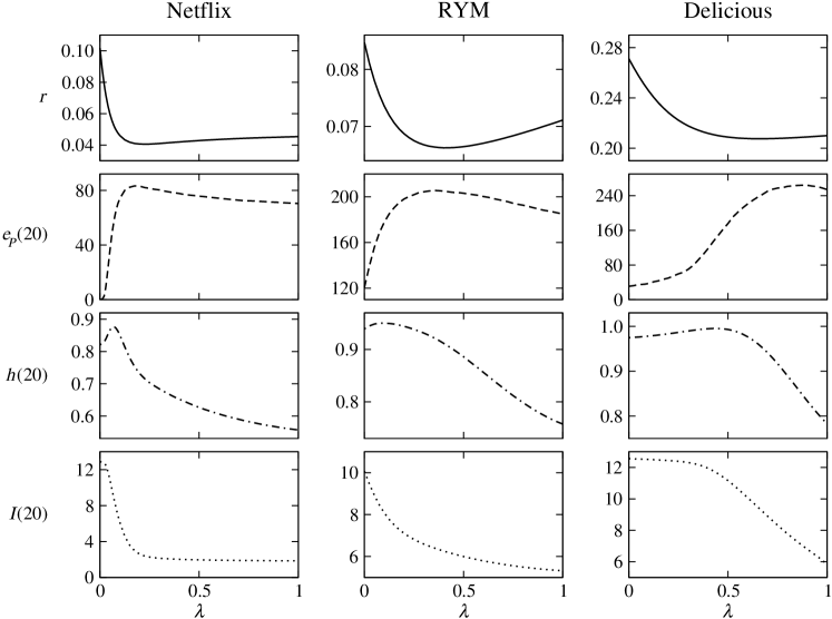
Figure 2: Performance of the HeatS+ProbS hybrid algorithm (Eq. 6) on the three different datasets. By varying the hybridization parameter between pure HeatS ($\lambda=0$) and pure ProbS ($\lambda=1$) it is possible to gain simultaneous performance enhancements with respect to both accuracy ($r$ and $e_{P}(L)$) and diversity ($h(L)$ and $I(L)$) of recommendations. Tuning $\lambda$ in this fashion allows the algorithm to be customized and optimized for different user or community needs.

Given that different algorithms serve different purposes and needs, is it possible to combine two (or more) in such a way as to obtain the best features of both? With HeatS favoring diversity and ProbS accuracy, their hybrid combination (Eq. 6) might be expected to provide a smooth transition from one to the other. In fact, the situation is even more favorable: while pure HeatS represents the optimum for novelty, it is possible to obtain performance improvements relative to all other metrics by tuning the hybridization parameter $\lambda$ appropriately (Fig. 2). The accuracy of ProbS can thus be maintained and even improved while simultaneously attaining diversity close to or even exceeding that of HeatS. Alternatively, diversity can be favored while minimizing the cost in terms of accuracy.

Depending on the particular needs of a system and its users, one can define an arbitrary utility function $U(r,e_{P},h,I,L)$ and choose $\lambda$ to optimize it: Table 4 gives as an example the percentage improvements that can be made, relative to pure ProbS ($\lambda=1$), if we choose $\lambda$ to minimize $r$. Shared improvements are obtained for all metrics except with the Delicious dataset, where minimizing $r$ has a negative effect on $e_{P}(L)$. However, from Fig. 2 we can see that even in this case it is possible to choose a value of $\lambda$ to simultaneously improve all metrics relative to ProbS.

Although HeatS+ProbS provides the best performance when taking into account all the metrics, other hybrids (constructed using the more general method of Eq. 5) can provide some valuable individual contributions (Fig. S7). HeatS+USim behaves similarly to HeatS+ProbS, but with generally smaller performance improvements. A more interesting hybrid is to combine the poorly-performing GRank with either HeatS or ProbS. These combinations can have a dramatic effect on link recovery: for RYM either can be tuned to produce an improvement in $r$ of almost 30% (relative to pure ProbS), compared to only 6.8% for the HeatS+ProbS hybrid (Table 4).

The explanation for these improvements stems from the way in which ProbS and HeatS interact with sparse datasets. Coverage of uncollected objects is limited to those sharing a user in common with an object collected by the target user (Fig. 1): all others receive a score of zero and so share a common (and large) relative rank, $r_{\alpha i}=(o-\frac{1}{2}(Z-1))/(o-k_{i})$ where $Z$ is the number of objects with zero score. GRank, with its universal coverage, is able to differentially rank these objects and so lower their contributions to $r$. Consequently, while incorporating it too strongly has a deleterious effect on the other metrics, a small GRank contribution can provide a useful enhancement to recommendation coverage—notably in “cold start” cases where little or nothing is known about a user.

3 Discussion

Recommender systems have at their heart some very simple and natural social processes. Each one of us looks to others for advice and opinions, learning over time who to trust and whose suggestions to discount. The paradox is that many of the most valuable contributions come not from close friends but from people with whom we have only a limited connection—“weak ties” who alert us to possibilities outside our regular experience [31].

The technical challenges facing recommender systems involve similar paradoxes. The most reliably accurate algorithms are those based on similarity and popularity of users and objects, yet the most valuable recommendations are those of niche items users are unlikely to find for themselves [21]. In this paper we have shown how this apparent dilemma can be resolved by an appropriate combination of diversity- and accuracy-focused methods, using a hybrid algorithm that joins a method with proven high accuracy with a new algorithm dedicated specifically to the production of novel and personalized recommendations. Their combination allows not merely a compromise between the two imperatives but allows us to simultaneously increase both accuracy and diversity of recommendations. By tuning the degree of hybridization the algorithms can be tailored to many custom situations and requirements.

We expect these results to be general: while we have presented a particular set of algorithms and datasets here, other recommender systems must face the same apparent dilemma and we expect them to benefit from a similar hybrid approach. It is interesting to note that while the Netflix Prize focused solely on accuracy, the winning entry in fact took a diversification approach, in this case based on tracking the changes in user opinions over time [32].

The algorithms presented here rely on no more than unary data and can thus place diversity at the heart of the recommendation process while still being applicable to virtually any dataset. More detailed sources of information can nevertheless be used to extend the recommendation process. Topical information and other measures of item-item similarity can be used to further diversify recommendation lists [24]: user-generated classifications such as tags [33, 34, 35] may be useful here. The HeatS and ProbS algorithms, and hence their hybrid, can be further customized by modifying the initial allocation of resource [36] to increase or decrease the influence of selected objects on the recommendation process. The hybridization process itself can be extended by incorporating techniques such as content-based or semantic analyses [23].

The ultimate measure of success for any recommender system is of course in the appreciation of its users, and in particular the ability of the system to serve their often very distinct needs. While in this paper we have optimized the hybrid from a global perspective, there is no reason why it cannot be tuned differently for each individual user—either by the system provider or by users themselves. This last consideration opens the door to extensive future theoretical and empirical research, bringing diversity and personalization not just to the contents of recommendation lists, but to the recommendation process itself.

Figure 1: The HeatS (a,b,c) and ProbS (d,e,f) algorithms (Eqs. 1 and 2) at work on the bipartite user-object network. Objects are shown as squares, users as circles, with the target user indicated by the shaded circle. While the HeatS algorithm redistributes resource via a nearest-neighbour averaging process, the ProbS algorithm works by an equal distribution of resource among nearest neighbours.

Table 1: Properties of the tested datasets.

dataset	users	objects	links	sparsity
Netflix	10 000	6 000	701 947	$1.17\cdot 10^{-2}$
RYM	33 786	5 381	613 387	$3.37\cdot 10^{-3}$
Delicious	10 000	232 657	1 233 997	$5.30\cdot 10^{-4}$

Table 2: Performance of the recommendation algorithms according to each of the four metrics: recovery of deleted links, precision enhancement, personalization, and surprisal.

	Netflix				RYM				Delicious
method	$r$	$e_{P}(20)$	$h(20)$	$I(20)$	$r$	$e_{P}(20)$	$h(20)$	$I(20)$	$r$	$e_{P}(20)$	$h(20)$	$I(20)$
GRank	0.057	58.7	0.450	1.79	0.119	57.3	0.178	4.64	0.314	147	0.097	4.23
USim	0.051	68.5	0.516	1.82	0.087	150	0.721	5.17	0.223	249	0.522	4.49
ProbS	0.045	70.4	0.557	1.85	0.071	185	0.758	5.32	0.210	254	0.783	5.81
HeatS	0.102	0.11	0.821	12.9	0.085	121	0.939	10.1	0.271	30.8	0.975	12.6

Table 3: Performance of individual recommendation algorithms for a probe set consisting of only low-degree ($k<100$) objects.

method	$r$	$e_{P}(20)$	$h(20)$	$I(20)$
GRank	0.327	0.000	0.525	1.68
USim	0.308	0.000	0.579	1.72
ProbS	0.279	0.014	0.610	1.74
HeatS	0.262	0.679	0.848	13.1

Table 4: Tuning the HeatS+ProbS hybridization parameter $\lambda$ to optimize for $r$ produces simultaneous improvements in other metrics. The relative changes are given in percentage terms against the pure ProbS algorithm.

dataset	$\lambda$	$\delta r$	$\delta e_{P}(20)$	$\delta h(20)$	$\delta I(20)$
Netflix	0.23	10.6%	16.5%	28.5%	28.8%
RYM	0.41	6.8%	10.8%	20.1%	17.2%
Delicious	0.66	1.2%	-6.0%	22.5%	61.7%

Supporting information
Zhou et al., “Solving the apparent diversity-accuracy dilemma
of recommender systems”

Figure S1. Elegant hybrids of the HeatS and ProbS algorithms can be created in several ways besides that given in Eq. 6 of the paper: for example $W_{\alpha\beta}^{\prime}=\big{(}\frac{1-\lambda}{k_{\alpha}}+\frac{\lambda}{k_{\beta}}\big{)}\sum_{j=1}^{u}a_{\alpha j}a_{\beta j}/k_{i}$, or $W_{\alpha\beta}^{\prime\prime}=\frac{1}{(1-\lambda)k_{\alpha}+\lambda k_{\beta}}\sum_{j=1}^{u}a_{\alpha j}a_{\beta j}/k_{j}$. While $W_{\alpha\beta}^{\prime}$ performs well only with respect to $I(20)$, Eq. 6 and $W_{\alpha\beta}^{\prime\prime}$ both have their advantages. However, Eq. 6 is somewhat easier to tune to different requirements since it varies more slowly and smoothly with $\lambda$. The results shown here are for the RateYourMusic dataset.

Figure S2. Precision $P(L)$ and recall $R(L)$ provide complementary but contrasting measures of accuracy: the former considers what proportion of selected objects (in our case, objects in the top $L$ places of the recommendation list) are relevant, the latter measures what proportion of relevant objects (deleted links) are selected. Consequently, recall (red) grows with $L$, whereas precision (blue) decreases. Here we compare precision and recall for the HeatS+ProbS hybrid algorithm on the Delicious and Netflix datasets. While quantitatively different, the qualitative performance is very similar for both measures.

Figure S3. A more elegant comparison can be obtained by considering precision and recall enhancement, that is, their values relative to that of randomly-sorted recommendations: $e_{P}(L)=P(L)\cdot ou/D$ and $e_{R}(L)=R(L)\cdot o/L$ (Eqs. 7a, b in the paper). Again, qualitative performance is close, and both of these measures decrease with increasing $L$, reflecting the inherent difficulty of improving either measure given a long recommendation list.

Figure S4. Comparison of the diversity-related metrics $h(20)$ and $I(20)$ when two different averaging procedures are used: averaging only over users with at least one deleted link (as displayed in the paper) and averaging over all users. The different procedures do not alter the results qualitatively and make little quantitative difference. The results shown are for the RateYourMusic dataset.

Figure S5. Comparison of performance metrics for different lengths $L$ of recommendation lists: $L=10$ (red), $L=20$ (green) and $L=50$ (blue). Strong quantitative differences are observed for precision enhancement $e_{P}(L)$ and personalization $h(L)$, but their qualitative behaviour remains unchanged. Much smaller differences are observed for surprisal $I(L)$.

Figure S6. Our accuracy-based metrics all measure in one way or another the recovery of links deleted from the dataset. Purely random deletion will inevitably favor high-degree (popular) objects, with their greater proportion of links, and consequently methods that favor popular items will appear to provide higher accuracy. To study this effect, we created two special probe sets consisting of links only to objects whose degree was less than some threshold (either 100 or 200): links to these objects were deleted with probability $0.5$, while links to higher-degree objects were left untouched. The result is a general decrease in accuracy for all algorithms—unsurprisingly, since rarer links are inherently harder to recover—but also a reversal of performance, with the low-degree-favoring HeatS now providing much higher accuracy than the high-degree-oriented ProbS, USim and GRank. The results shown here are for the Netflix dataset.

Figure S7. In addition to HeatS+ProbS, various other hybrids were created and tested using the method of Eq. 5 in the paper, where for hybrid X+Y, $\lambda=0$ corresponds to pure X and $\lambda=1$ pure Y. The results shown here are for the Netflix dataset. The HeatS+USim hybrid offers similar but weaker performance compared to HeatS+ProbS; combinations of GRank with other methods produce significant improvements in $r$, the recovery of deleted links, but show little or no improvement of precision enhancement $e_{P}(L)$ and poor results in diversity-related metrics. We can conclude that the proposed HeatS+ProbS hybrid is not only computationally convenient but also performs better than combinations of the other methods studied.