Cosmology-Independent Distance Moduli of 42 Gamma-Ray Bursts between Redshift of 1.44 and 6.60

Abstract

This report is an update and extension of our paper accepted for publication in ApJ (arXiv:0802.4262). Since objects at the same redshift should have the same luminosity distance and the distance moduli of type Ia supernovae (SNe Ia) obtained directly from observations are completely cosmology independent, we obtain the distance modulus of a gamma-ray burst (GRB) at a given redshift by interpolating or iterating from the Hubble diagram of SNe Ia. Then we calibrate five GRB relations without assuming a particular cosmological model, from different regression methods, and construct the GRB Hubble diagram to constrain cosmological parameters. Based upon these relations we list the cosmology-independent distance moduli of 42 GRBs between redshift of 1.44 and 6.60, with the 1-$\sigma$ uncertainties of 1-3%.

1 Introduction

Gamma-ray burst (GRB) luminosity/energy relations are connections between measurable properties of the prompt gamma-ray emission with the luminosity or energy. In recent years, several empirical GRB luminosity relations as standard candles for cosmology research at very high redshift have been proposed GRB2008 , Schaefer2007 . An important concern in the application of GRBs to cosmology is the dependence on the cosmological model in the calibration of GRB relations in many works. For the difficulty to calibrate the relations with a low-redshift sample, GRB relations have usually been calibrated by assuming a particular cosmological model. Therefore the circularity problem can not be avoided easily. Many previous works treated the circularity problem by means of statistical approaches. However, we note that the circularity problem is not circumvented completely by means of statistical approaches, because a particular cosmology model is required in doing the joint fitting.

In this report, we present two new methods (interpolation method and iterative method) to calibrate the GRB relations in a cosmological model-independent way. This report is an update and extension of our paper accepted for publication in ApJLiang2008 . It is obvious that objects at the same redshift should have the same luminosity distance in any cosmology. There are so many SNe Ia that we can obtain the luminosity distance (also the distance moduli) at any redshift in the redshift range of SNe Ia by interpolating from SN Ia data. Recently, on the basis of smoothing the noise of supernova data over redshift, the authors in Shafieloo2006 ,Wu2008 suggested a non-parametric method in a model independent manner to reconstruct the luminosity distance at any redshift in the redshift range of SNe Ia by the iterative method. Furthermore, the luminosity distance of SNe Ia obtained directly from observations are completely cosmological model independent. Therefore, we can obtain the distance moduli of GRBs in the redshift range of SNe Ia and calibrate GRB relations in a completely cosmological model independent way and use the standard Hubble diagram method to constrain the cosmological parameters from GRB data at high redshift obtained by utilizing the relations.

2 cosmological model independent High-z GRB distance moduli

We first calibrate five GRB luminosity/energy relations with the sample at $z\leq 1.4$, i.e., the luminosity ($L$)-spectral lag ($\tau_{\rm lag}$) relation Norris2000 , the $L$-variability ($V$) relation Fenimore2000 , the $L$-$E_{\rm p}$ relation Schaefer2003 , the collimation-corrected energy ($E_{\gamma}$)-$E_{\rm p}$ relation Ghirlanda2004 , the $\tau_{\rm RT}$-$L$ relation Schaefer2007 , where $\tau_{\rm RT}$ is the minimum rise time in the GRB light curve. A GRB luminosity relation can be generally written in the form of

$$\log y=a+b\log x,$$ (1)

where $a$ and $b$ are the intercept and slope of the relation respectively; $y$ is the luminosity ($L$ in units of $\rm erg\ s^{-1}$) or the collimation-corrected energy ($E_{\gamma}$ in units of $\rm erg$); $x$ is the GRB parameters measured in the rest frame, e.g., $\tau_{\rm lag}(1+z)^{-1}/(0.1\rm\ s)$, $V(1+z)/0.02$, $E_{\rm p}(1+z)/(300\ \rm keV)$, $\tau_{\rm RT}(1+z)^{-1}/\rm(0.1\ s)$. (We adopt the data of these quantities from Ref. Schaefer2007 .)

We adopt the data of 192 SNe Ia Davis2007 and show them in Figure 1. There is only one SN Ia point (the redshift of SN1997ff is $z=1.755$) at $z>1.4$, therefore we exclude it from our SN Ia sample used to interpolate the distance moduli of GRBs in the redshift range of SN Ia sample.

FIGURE 1. The Hubble Diagram of 192 SNe Ia (red dots) and the 69 GRBs obtained by using the cosmology-independent methods. The 27 GRBs at $z\leq 1.4$ are obtained by using the interpolation and iterative methods directly from SN Ia data; and the 42 GRBs at $z>1.4$ are obtained by utilizing the five relations calibrated with the sample at $z\leq 1.4$ using by the cosmology-independent methods (black circles: the interpolation method; blue stars: the iterative method). The curve is the theoretical distance modulus in the concordance model ($w_{0}=-1$, $\Omega_{\rm M}=0.27$, $\Omega_{\Lambda}=0.73$), and the vertical dotted line represents $z=1.4$.

Following a well known procedure in the analysis of large scale structure, Shafieloo et al Shafieloo2006 used a Gaussian smoothing function rather than the top hat smoothing function to smooth the noise of the Sne Ia data directly. In order to obtain important information on interesting cosmological parameters expediently, when doing the Gaussian smoothingShafieloo2006 $\ln d_{L}(z)$, rather than the luminosity distance $d_{L}(z)$ or distance modulus $\mu(z)$, is studied by the iterative method. We thus follow the iterative procedure and adopt the results from Ref. Wu2008 ,

$$\ln d_{L}(z)^{s}_{n}=\ln d_{L}(z)^{s}_{n-1}+N(z)\sum_{i}(\ln d^{obs}_{L}(z_{i})-\ln d_{L}(z_{i})^{s}_{n-1})\exp\big{[}-\big{(}\ln^{2}\big{(}(1+z)/(1+z_{i})\big{)}\big{)}/\big{(}2\triangle^{2}\big{)}\big{]},$$ (2)

with a normalization parameter $N(z)^{-1}=\sum_{i}\exp\big{[}-\big{(}\ln^{2}\big{(}(1+z)/(1+z_{i})\big{)}\big{)}/\big{(}2\triangle^{2}\big{)}\big{]}$, and $\triangle=0.6$. $d_{L}(z)^{s}_{n}$ represents the smoothed luminosity distance at any redshift $z$ after the $n$th iteration and $d_{L}(z)^{s}_{0}$ denotes a guess background model. It has been shown that the results are not sensitive to the chosen vaule of $\Delta$ and the assumed initial guess model. $d^{obs}_{L}(z_{i})$ is the observed one from the SN Ia data. The best fitting result is obtained by minimizing $\chi^{2}_{n}=\sum_{i}(\mu(z_{i})_{n}-\mu^{obs}(z_{i}))^{2}/\sigma^{2}_{\mu_{obs,i}}\;$.

The isotropic luminosity of a burst is calculated by $L=4\pi d_{\rm L}^{2}P_{\rm bolo}$, where $d_{\rm L}$ is the luminosity distance of the burst and $P_{\rm bolo}$ is the bolometric flux of gamma-rays in the burst. The isotropic energy released from a burst is given by $E_{\rm iso}=4\pi d_{\rm L}^{2}S_{\rm bolo}(1+z)^{-1},$ where $S_{\rm bolo}$ is the bolometric fluence of gamma-rays in the burst at redshift $z$. The total collimation-corrected energy is then calculated by $E_{\gamma}=F_{\rm beam}E_{\rm iso},$ where the beaming factor, $F_{\rm beam}$ is $(1-\cos\theta_{\rm jet})$ with the jet opening angle ($\theta_{\rm jet}$), which is related to the break time ($t_{\rm b}$).

We determine the values of the intercept ($a$) and the slope ($b$) calibrated with the GRB sample at $z\leq 1.4$ by using the interpolationLiang2008 and iterativeWu2008 methods, respectively. We first use the same regression method as used in Ref.Schaefer2007 : the bisector of the two ordinary least-squares(OLS) linear regressions, which has been discussed in Ref.Isobe1990 , OLS(Y—X) (OLS regression of the dependent variable Y against the independent variable X) and its inverse OLS(X—Y). In order to avoid specifying “dependent” and “independent” variables, the OLS(Y—X) and the OLS(X—Y) lines should be bisected. The OLS regressions does not take the errors into account; but the use of weighted least-squares(WLS), taking into account the measurable uncertainties, results in almost identical best fits. Therefore, the WLS bisector regression can be obtained by bisecting the WLS(Y—X) and the WLS(X—Y) lines. The calibration results from two regression methods (the OLS bisector and the WLS bisector) are summarized in Table 1 and we also list the results calibrated with the same sample ($z\leq 1.4$) by assuming the $\Lambda$CDM model for comparison. From Table 1, we find that results from the two regression methods make no significant difference from each other. Therefore, taking into account the measurement uncertainties in the regression, indeed will not change the fitting parameters significantly, when the measurement uncertainties are smaller than the intrinsic error Schaefer2007 . We also find that results obtained by assuming the $\Lambda$CDM with the same sample differ only slightly from, but still fully consistent with those calibrated by using our interpolation method. The reason for this is easy to understand, since the $\Lambda$CDM is fully compatible with SN Ia data. Nevertheless, it should be noticed that the calibration results obtained by using the interpolation or iterative method directly from SN Ia data are completely cosmology independent.

	Interpolation method		Iterative method		$\Lambda$CDM model
	$a$	$b$	$a$	$b$	$a$	$b$
$\tau_{\rm lag}$-$L$ relation	52.22$\pm 0.09$	-1.07$\pm 0.13$	52.22$\pm 0.09$	-1.10$\pm 0.14$	52.15$\pm 0.10$	-1.11$\pm 0.14$
	52.22$\pm 0.09$	-1.07$\pm 0.14$	52.22$\pm 0.09$	-1.10$\pm 0.15$	52.14$\pm 0.10$	-1.10$\pm 0.14$
$V$-$L$ relation	52.59$\pm 0.13$	2.05$\pm 0.27$	52.56$\pm 0.13$	2.03$\pm 0.30$	52.48$\pm 0.13$	2.04$\pm 0.30$
	52.59$\pm 0.13$	2.08$\pm 0.37$	52.57$\pm 0.13$	2.10$\pm 0.42$	52.49$\pm 0.13$	2.11$\pm 0.42$
$L$-$E_{\rm p}$ relation	52.26$\pm 0.09$	1.69$\pm 0.11$	52.23$\pm 0.09$	1.65$\pm 0.12$	52.15$\pm 0.09$	1.66$\pm 0.12$
	52.26$\pm 0.09$	1.69$\pm 0.16$	52.23$\pm 0.09$	1.65$\pm 0.16$	52.15$\pm 0.09$	1.65$\pm 0.16$
$E_{\gamma}$-$E_{\rm p}$ relation	50.71$\pm 0.07$	1.79$\pm 0.18$	50.68$\pm 0.06$	1.75$\pm 0.18$	50.59$\pm 0.06$	1.75$\pm 0.19$
	50.71$\pm 0.06$	1.68$\pm 0.29$	50.68$\pm 0.06$	1.63$\pm 0.30$	50.60$\pm 0.06$	1.64$\pm 0.30$
$\tau_{\rm RT}$-$L$ relation	52.64$\pm 0.11$	-1.32$\pm 0.15$	52.60$\pm 0.10$	-1.30$\pm 0.15$	52.52$\pm 0.11$	-1.30$\pm 0.15$
	52.64$\pm 0.11$	-1.33$\pm 0.16$	52.60$\pm 0.10$	-1.31$\pm 0.16$	52.52$\pm 0.11$	-1.31$\pm 0.17$

Table 1: Calibration results ($a$: intercept, $b$: slope) with their 1-$\sigma$ uncertainties for the five GRB luminosity/energy relations with the sample at $z\leq 1.4$, by using the interpolation and iterative methods directly from SNe Ia data, and by assuming a particular cosmological models (the $\Lambda$CDM model). Only the data available from Table 4 in Ref.Schaefer2007 are used to calibrate the five GRB relations. For each relation, the results on the first and second lines are calibrated from the OLS and WLS bisector regressions, respectively.

By utilizing the calibrated relations at high redshift ($z>1.4$), we are able to obtain the luminosity ($L$) or energy ($E_{\gamma}$) of each burst at $z>1.4$. We use the same method used in Ref.Schaefer2007 to obtain the best estimate $\mu$ for each GRB which is the weighted average of all available distance moduli. The derived distance modulus for each GRB is

$$\mu=(\sum_{i}\mu_{\rm i}/\sigma_{\mu_{\rm i}}^{2})/(\sum_{i}\sigma_{\mu_{\rm i}}^{-2}),$$ (3)

with its uncertainty $\sigma_{\mu}=(\sum_{i}\sigma_{\mu_{\rm i}}^{-2})^{-1/2}$, where the summations run from 1 to 5 over the five relations used in Schaefer (2007) with available data.

We plot the Hubble diagram of the 69 GRBs obtained by using the interpolation and iterative methods in Figure 1. The 27 GRBs at $z\leq 1.4$ are obtained by using the interpolation and iterative methods directly from SNe data. The distance moduli of these 42 GRBs at $z>1.4$ are obtained by utilizing the five relations calibrated with the sample at $z\leq 1.4$ using the cosmology-independent methods. The derived distance moduli for the 42 GRBs ($z>1.4$) with different methods are listed in Table 2, together with the average values between different methods, which should be the least biased and most robust values to be used to study the expansion history of the Universe up to $z=6.60$. It should be noted that the 1-$\sigma$ uncertainties listed in Table 2, ranging between 1% to 3%, include both the measurement uncertainties and intrinsic scattering in these luminosity/energy relations.

	GRB	$z$	$\mu_{1}^{a}$	$\mu_{1}^{b}$	$\mu_{2}^{a}$	$\mu_{2}^{b}$	$\mu$
	050318	1.44	45.86 $\pm$ 0.58	45.91 $\pm$ 0.59	45.80 $\pm$ 0.57	45.86 $\pm$ 0.58	45.86 $\pm$ 0.58
	010222	1.48	44.87 $\pm$ 0.51	44.77 $\pm$ 0.53	44.73 $\pm$ 0.51	44.63 $\pm$ 0.53	44.75 $\pm$ 0.52
	060418	1.49	45.46 $\pm$ 0.63	45.46 $\pm$ 0.63	45.43 $\pm$ 0.63	45.43 $\pm$ 0.63	45.45 $\pm$ 0.63
	060502	1.51	44.61 $\pm$ 0.75	44.62 $\pm$ 0.76	44.57 $\pm$ 0.75	44.58 $\pm$ 0.75	44.60 $\pm$ 0.75
	030328	1.52	44.99 $\pm$ 0.54	44.99 $\pm$ 0.54	44.92 $\pm$ 0.54	44.92 $\pm$ 0.53	44.96 $\pm$ 0.54
	051111	1.55	43.90 $\pm$ 0.77	43.89 $\pm$ 0.77	43.82 $\pm$ 0.77	43.81 $\pm$ 0.77	43.85 $\pm$ 0.77
	990123	1.61	45.15 $\pm$ 0.53	44.98 $\pm$ 0.56	45.06 $\pm$ 0.53	44.89 $\pm$ 0.55	45.02 $\pm$ 0.54
	990510	1.62	45.76 $\pm$ 0.47	45.75 $\pm$ 0.47	45.69 $\pm$ 0.46	45.69 $\pm$ 0.46	45.72 $\pm$ 0.46
	050802	1.71	45.67 $\pm$ 1.34	45.67 $\pm$ 1.34	45.60 $\pm$ 1.30	45.60 $\pm$ 1.31	45.64 $\pm$ 1.32
	030226	1.98	46.70 $\pm$ 0.54	46.70 $\pm$ 0.54	46.63 $\pm$ 0.54	46.64 $\pm$ 0.54	46.67 $\pm$ 0.54
	060108	2.03	47.60 $\pm$ 1.21	47.60 $\pm$ 1.21	47.54 $\pm$ 1.19	47.54 $\pm$ 1.19	47.57 $\pm$ 1.20
	000926	2.07	45.84 $\pm$ 0.85	45.85 $\pm$ 0.85	45.74 $\pm$ 0.83	45.76 $\pm$ 0.84	45.80 $\pm$ 0.84
	011211	2.14	45.85 $\pm$ 0.64	45.90 $\pm$ 0.64	45.81 $\pm$ 0.63	45.86 $\pm$ 0.63	45.85 $\pm$ 0.63
	050922	2.20	46.13 $\pm$ 0.65	46.13 $\pm$ 0.65	46.10 $\pm$ 0.64	46.10 $\pm$ 0.65	46.12 $\pm$ 0.65
	060124	2.30	47.29 $\pm$ 0.52	47.24 $\pm$ 0.52	47.20 $\pm$ 0.51	47.15 $\pm$ 0.52	47.22 $\pm$ 0.52
	021004	2.32	46.58 $\pm$ 0.59	46.58 $\pm$ 0.59	46.53 $\pm$ 0.58	46.53 $\pm$ 0.58	46.56 $\pm$ 0.59
	051109	2.35	45.94 $\pm$ 0.97	45.94 $\pm$ 0.98	45.85 $\pm$ 0.95	45.85 $\pm$ 0.95	45.90 $\pm$ 0.96
	050406	2.44	46.45 $\pm$ 0.80	46.45 $\pm$ 0.80	46.48 $\pm$ 0.79	46.47 $\pm$ 0.79	46.46 $\pm$ 0.79
	030115	2.50	46.43 $\pm$ 0.71	46.43 $\pm$ 0.71	46.39 $\pm$ 0.70	46.38 $\pm$ 0.71	46.41 $\pm$ 0.71
	050820	2.61	47.22 $\pm$ 0.96	47.21 $\pm$ 0.97	47.11 $\pm$ 0.94	47.10 $\pm$ 0.94	47.16 $\pm$ 0.95
	030429	2.66	46.56 $\pm$ 0.67	46.60 $\pm$ 0.67	46.50 $\pm$ 0.66	46.56 $\pm$ 0.66	46.56 $\pm$ 0.67
	060604	2.68	46.31 $\pm$ 0.72	46.33 $\pm$ 0.72	46.29 $\pm$ 0.71	46.31 $\pm$ 0.71	46.31 $\pm$ 0.72
	050603	2.82	45.70 $\pm$ 0.66	45.71 $\pm$ 0.67	45.61 $\pm$ 0.65	45.62 $\pm$ 0.66	45.66 $\pm$ 0.66
	050401	2.90	47.41 $\pm$ 0.70	47.42 $\pm$ 0.70	47.32 $\pm$ 0.69	47.34 $\pm$ 0.69	47.37 $\pm$ 0.70
	060607	3.08	46.32 $\pm$ 0.67	46.32 $\pm$ 0.67	46.27 $\pm$ 0.66	46.28 $\pm$ 0.66	46.30 $\pm$ 0.66
	020124	3.20	47.23 $\pm$ 0.51	47.22 $\pm$ 0.50	47.16 $\pm$ 0.50	47.15 $\pm$ 0.50	47.19 $\pm$ 0.50
	060526	3.21	47.52 $\pm$ 0.53	47.58 $\pm$ 0.54	47.49 $\pm$ 0.53	47.55 $\pm$ 0.53	47.53 $\pm$ 0.53
	050319	3.24	48.49 $\pm$ 1.26	48.51 $\pm$ 1.26	48.41 $\pm$ 1.22	48.44 $\pm$ 1.23	48.46 $\pm$ 1.24
	050908	3.35	47.05 $\pm$ 0.95	47.05 $\pm$ 0.95	47.00 $\pm$ 0.92	47.00 $\pm$ 0.92	47.03 $\pm$ 0.93
	030323	3.37	47.23 $\pm$ 1.20	47.23 $\pm$ 1.20	47.17 $\pm$ 1.17	47.17 $\pm$ 1.17	47.20 $\pm$ 1.19
	971214	3.42	48.71 $\pm$ 0.74	48.72 $\pm$ 0.74	48.63 $\pm$ 0.73	48.65 $\pm$ 0.74	48.67 $\pm$ 0.74
	060115	3.53	48.01 $\pm$ 0.97	48.01 $\pm$ 0.97	47.93 $\pm$ 0.95	47.94 $\pm$ 0.95	47.97 $\pm$ 0.96
	050502	3.79	46.34 $\pm$ 0.67	46.30 $\pm$ 0.68	46.30 $\pm$ 0.67	46.26 $\pm$ 0.67	46.30 $\pm$ 0.67
	060605	3.80	47.09 $\pm$ 0.81	47.09 $\pm$ 0.82	47.06 $\pm$ 0.80	47.05 $\pm$ 0.81	47.07 $\pm$ 0.81
	060210	3.91	48.35 $\pm$ 0.53	48.29 $\pm$ 0.54	48.27 $\pm$ 0.53	48.21 $\pm$ 0.53	48.28 $\pm$ 0.53
	060206	4.05	46.82 $\pm$ 0.75	46.81 $\pm$ 0.76	46.75 $\pm$ 0.74	46.75 $\pm$ 0.75	46.78 $\pm$ 0.75
	050505	4.27	48.08 $\pm$ 0.69	48.10 $\pm$ 0.69	47.99 $\pm$ 0.68	48.00 $\pm$ 0.68	48.04 $\pm$ 0.69
	060223	4.41	47.89 $\pm$ 0.66	47.89 $\pm$ 0.66	47.85 $\pm$ 0.65	47.85 $\pm$ 0.65	47.87 $\pm$ 0.66
	000131	4.50	48.02 $\pm$ 0.84	48.03 $\pm$ 0.84	47.92 $\pm$ 0.83	47.94 $\pm$ 0.83	47.98 $\pm$ 0.84
	060510	4.90	48.90 $\pm$ 1.15	48.90 $\pm$ 1.16	48.82 $\pm$ 1.13	48.83 $\pm$ 1.14	48.86 $\pm$ 1.14
	050904	6.29	49.91 $\pm$ 0.65	49.75 $\pm$ 0.71	49.74 $\pm$ 0.65	49.58 $\pm$ 0.71	49.74 $\pm$ 0.68
	060116	6.60	48.59 $\pm$ 1.08	48.59 $\pm$ 1.08	48.48 $\pm$ 1.05	48.47 $\pm$ 1.06	48.53 $\pm$ 1.07

Table 2: Cosmology-independent distance moduli of 42 GRB ($1.44\leq z\leq 6.60$). $\mu_{1}$ and $\mu_{2}$ are obtained by the interpolation and iterative methods, respectively; $\mu^{a}$ and $\mu^{b}$ are obtained from the OLS and WLS bisector regressions, respectively. $\mu=(\mu_{1}^{a}+\mu_{1}^{b}+\mu_{2}^{a}+\mu_{2}^{b})/4$ and $\sigma_{\mu}=(\sigma_{\mu_{1}^{a}}+\sigma_{\mu_{1}^{b}}+\sigma_{\mu_{2}^{a}}+\sigma_{\mu_{2}^{b}})/4$, which should be least biased and most robust for applications. The 1-$\sigma$ uncertainties include both the measurement uncertainties and intrinsic scattering in these luminosity/energy relations.

In Figure 2 we show examples of cosmological parameter fitting by the minimum $\chi^{2}$ method. Figure 2a and b show the joint confidence regions for ($\Omega_{\rm M},\Omega_{\Lambda}$) in the $\Lambda$CDM model from the distance moduli of these 42 GRBs ($z>1.4$) obtained by utilizing the five relations calibrated with the sample at $z\leq 1.4$, using the interpolation and iterative methods, respectively. Figure 2c and d represent the contours of likelihood in the ($\Omega_{\rm M},w_{0}$) plane in the dark energy model with a constant $w_{0}$ for a flat universe. Here we adopt $H_{0}=70\ \rm km\ s^{-1}Mpc^{-1}$. All fitted parameters are listed in Table 3. We find that the fitting results from the OLS regression differ only slightly from, but still fully consistent with those from the WLS regression. But the use of WLS, taking into account the measurement uncertainties in the regression, results in almost identical best fits.

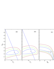
Figure 2: (a) and (b) Joint confidence regions for ($\Omega_{\rm M},\Omega_{\Lambda}$) in the $\Lambda$CDM model from the data for 42 GRBs ($z>1.4$) obtained by utilizing the five relations calibrated with the sample at $z\leq 1.4$, using the interpolation and iterative methods, respectively. The dashed line represents the flat universe. (c) and (d) Contours of likelihood in the ($\Omega_{\rm M},w_{0}$) plane in the dark energy model with a constant $w_{0}$ for a flat universe. For each panel, the horizontal line is for a prior of $\Omega_{\rm M}=0.27$. For all four panels, the plus sign indicates the best-fit values and the contours correspond to 1, 2, and 3-$\sigma$ confidence regions. The numerical values of fitted parameters are listed in Table 3.

	OLS(Y—X)	WLS(Y—X)	OLS(X—Y)	WLS(X—Y)	OLS Bisector	WLS Bisector
$\Omega_{\rm M}$	$0.35_{-0.05}^{+0.06}$	$0.35_{-0.06}^{+0.06}$	$0.18_{-0.07}^{+0.05}$	$0.21_{-0.07}^{+0.06}$	$0.27_{-0.06}^{+0.05}$	$0.28_{-0.06}^{+0.05}$
	$0.38_{-0.07}^{+0.07}$	$0.38_{-0.05}^{+0.07}$	$0.21_{-0.08}^{+0.05}$	$0.24_{-0.08}^{+0.06}$	$0.30_{-0.06}^{+0.06}$	$0.31_{-0.06}^{+0.06}$
$w_{0}$	$-0.72_{-0.30}^{+0.21}$	$-0.73_{-0.31}^{+0.23}$	$-1.51_{-1.20}^{+0.50}$	$-1.29_{-0.96}^{+0.43}$	$-0.97_{-0.48}^{+0.28}$	$-0.94_{-0.45}^{+0.27}$
	$-0.63_{-0.25}^{+0.21}$	$-0.63_{-0.26}^{+0.20}$	$-1.25_{-0.75}^{+0.39}$	$-1.09_{-0.66}^{+0.35}$	$-0.84_{-0.36}^{+0.24}$	$-0.82_{-0.36}^{+0.24}$

Table 3: The cosmological fitting results from the distance moduli of these 42 GRBs ($z>1.4$) obtained utilizing the five relations calibrated with the sample at $z\leq 1.4$ using the interpolation and iterative methods, from different linear regressions. The fitted $\Omega_{\rm M}$ is for the flat $\Lambda$CDM model. For the dark energy model with a constant equation of state $w_{0}$ is for a prior of $\Omega_{\rm M}=0.27$. For the every two lines of each parameter, the results on the first line are derived from the interpolation method, and that on the second line are from the iterative method.

3 Summary

Since the distance modulus of any SN Ia is completely cosmological model independent, we can obtain the distance modulus of a GRB at a given redshift by interpolating or iterating from the Hubble diagram of SNe Ia at $z\leq 1.4$, in order to calibrate the GRB luminosity relations in a completely cosmology independent way. Since our method does not depend on a particular cosmological model when we calibrate the parameters of GRB luminosity relations, the so-called circularity problem can be completely avoided. With this method, we obtained the cosmology-independent distance moduli of 42 GRBs between redshift of 1.44 and 6.60, which are listed in Table 2.

With these cosmology-independent distance moduli of high redshift GRBs, we construct the GRB Hubble diagram and constrain cosmological parameters by the minimum $\chi^{2}$ method as in SN Ia cosmology. We obtain $\Omega_{\rm M}=0.28_{-0.06}^{+0.05}$, $\Omega_{\Lambda}=0.72_{-0.05}^{+0.06}$ for the flat $\Lambda$CDM model from the GRB data obtained by using the interpolation method, and $\Omega_{\rm M}=0.31_{-0.06}^{+0.06}$, $\Omega_{\Lambda}=0.69_{-0.06}^{+0.06}$ from the data obtained by using the iterative method. For the dark energy model with a constant equation of state, we obtain $w_{0}=-0.94_{-0.45}^{+0.27}$ and $w_{0}=-0.82_{-0.36}^{+0.24}$ for a flat universe from the data obtained by the two methods respectively, which is consistent with the concordance model within the statistical error. Our result suggests the the concordance model ($w_{0}=-1$, $\Omega_{\rm M}=0.27$, $\Omega_{\Lambda}=0.73$) is still consistent with the GRB data at higher redshift up to $z=6.6$.

References

- (1) Ghirlanda, G. et al. 2004, ApJ, 613, L13; Dai, Z. G., Liang, E. W., & Xu, D. 2004, ApJ, 612, L101; Firmani, C., Ghisellini, G., Ghirlanda, G., & Avila-Reese, V. 2005, MNRAS, 360, L1; Liang, E. W. & Zhang, B. 2005, ApJ, 633, 603; Firmani, C., Avila-Reese, V., Ghisellini, G., & Ghirlanda, G. 2006, MNRAS, 372, L28; Ghirlanda, G., Ghisellini, G., & Firmani, C. 2006, New J. Phys, 8, 123; Firmani, C., Avila-Reese, V., Ghisellini, G., & Ghirlanda, G. 2007, RMxAA, 43, 203; Kodama, Y. et al. 2008, MNRAS in press (arXiv:0802.3428); Amati, L. et al. 2008, arXiv:0805.0377; Basilakos, S. & Perivolaropoulos, L. 2008, arXiv:0805.0875; Capozziello, S. & Izzo, L. arXiv:0806.1120; Mosquera Cuesta, H. J. et al. 2008, A&A, 487, 47; Mosquera Cuesta, H. J. et al. 2008, JCAP, 0807, 04
- (2) Schaefer, B. E. 2007, ApJ, 660, 16
- (3) Liang, N., Xiao, W. K., Liu, Y., Zhang, S. N. 2008, ApJ, accepted for publication (arXiv:0802.4262)
- (4) Shafieloo, A., Alam, U., Sahni, V. and Starobinsky, A., 2006, MNRAS, 366, 1081; Shafieloo, A., 2007 MNRAS, 380, 1573
- (5) Wu, P. X. & Yu H. W. 2008, JCAP, 0802, 19
- (6) Norris, J. P., Marani, G. F., & Bonnell, J. T. 2000, ApJ, 534, 248
- (7) Fenimore, E. E. & Ramirez-Ruiz, E. 2000, astro-ph/0004176; Riechart, D. E., Lamb, D. Q., Fenimore, E. E., Ramirez-Ruiz, Cline, T. L., & Hurley, K. 2001, ApJ, 552, 57.
- (8) Schaefer, B. E. 2003, ApJ, 583, L71; Yonetoku, D. et al. 2004, ApJ, 609, 935
- (9) Ghirlanda, G., Ghisellini, G., & Lazzati, D. 2004, ApJ, 616, 331
- (10) Davis T. M. et al. 2007, ApJ, 666, 716; Astier, P., et al. 2006, A&A, 447, 31; Wood-Vasey, W. M. et al. 2007, ApJ, 666, 694; Riess, A. G. et al. 2007, ApJ, 659, 98
- (11) Isobe, T. et al. 1990, ApJ, 364, 304