The Chemical and Ionization Conditions in Weak Mg ii Absorbers

Abstract

We present an analysis of the chemical and ionization conditions in a sample of $100$ weak Mg ii absorbers identified in the VLT/UVES archive of quasar spectra. In addition to Mg ii, we present equivalent width and column density measurements of other low ionization species such as Mg i, Fe ii, Al ii, C ii, Si ii and also Al iii. We find that the column densities of C ii and Si ii are strongly correlated with the column density of Mg ii, with minimal scatter in the relationships. The column densities of Fe ii exhibit an appreciable scatter when compared with the column density of Mg ii, with some fraction of clouds having $N(\hbox{{\rm Fe~{}}\kern 1.00006pt{\sc ii}})\sim N(\hbox{{\rm Mg~{}}\kern 1.00006pt{\sc ii}})$, in which case the density is constrained to n${}_{\hbox{{\rm H}}}>0.05$ cm^-3. Other clouds in which $N(\hbox{{\rm Fe~{}}\kern 1.00006pt{\sc ii}})<<N(\hbox{{\rm Mg~{}}\kern 1.00006pt{\sc ii}})$ have much lower densities. From ionization models, we infer that the metallicity in a significant fraction of weak Mg ii clouds is constrained to values of solar or higher, if they are sub-Lyman limit systems. Based on the observed constraints, we hypothesize that weak Mg ii absorbers are predominantly tracing two different astrophysical processes/structures. A significant population of weak Mg ii clouds, those in which $N(\hbox{{\rm Fe~{}}\kern 1.00006pt{\sc ii}})<<N(\hbox{{\rm Mg~{}}\kern 1.00006pt{\sc ii}})$, identified at both low ($z\sim 1$) and high ($z\sim 2$) redshift, are likely to be tracing gas in the extended halos of galaxies, analogous to the Galactic high velocity clouds. These absorbers might correspond to $\alpha$-enhanced interstellar gas expelled from star-forming galaxies, in correlated supernova events. The $N(\hbox{{\rm Mg~{}}\kern 1.00006pt{\sc ii}})$ and $N(\hbox{{\rm Fe~{}}\kern 1.00006pt{\sc ii}})/N(\hbox{{\rm Mg~{}}\kern 1.00006pt{\sc ii}})$ in such clouds are also closely comparable to those measured for the high velocity components in strong Mg ii systems. An evolution is found in $N(\hbox{{\rm Fe~{}}\kern 1.00006pt{\sc ii}})/N(\hbox{{\rm Mg~{}}\kern 1.00006pt{\sc ii}})$ from $z=2.4$ to $z=0.4$, with an absence of weak Mg ii clouds with $N(\hbox{{\rm Fe~{}}\kern 1.00006pt{\sc ii}})\sim N(\hbox{{\rm Mg~{}}\kern 1.00006pt{\sc ii}})$ at high-$z$. The $N(\hbox{{\rm Fe~{}}\kern 1.00006pt{\sc ii}})\sim N(\hbox{{\rm Mg~{}}\kern 1.00006pt{\sc ii}})$ clouds, which are prevalent at lower redshifts ($z<1.5$), must be tracing Type Ia enriched gas in small, high metallicity pockets in dwarf galaxies, tidal debris, or other intergalactic structures.

1. INTRODUCTION

The H i gas directly associated with galaxies that intercept the line of sight to background quasars appears as optically thick Lyman Limit systems in the quasar spectrum. The prominent metal lines associated with these intervening absorbers are typically observed to be kinematically broad ($\Delta v\sim 100-400$ km s^-1), strong, and often saturated (e.g., Steidel & Sargent, 1992; Churchill & Vogt, 2001) . Studying the properties of a large population of such strong Mg ii absorbers is a technique used for constraining the evolution of metals in the interstellar media, gaseous halos and coronae of galaxies over a large history of the universe (Lanzetta et al., 1987; Churchill et al., 1996). Apparently distinct from these strong Mg ii absorbers are the population of quasar absorption line systems in which the low ionization metal lines are weak. These systems are separated from the strong ones based on the standard definition of the rest-frame equivalent width of $\hbox{{\rm Mg~{}}\kern 1.00006pt{\sc ii}}~{}\lambda 2796$ Å line being $W_{r}(2796)<0.3$ Å. This is not a firm criterion for division, but has been followed as a convention on the following basis. The survey of Steidel & Sargent (1992), which identified a large population of strong Mg ii absorbers used a sample of intermediate resolution spectra ($\Delta\lambda\sim 5$ Å) which had an equivalent width threshold of $\sim 0.3$ Å. Later surveys of higher sensitivity and spectral resolution found that the equivalent width distribution of Mg ii systems at $z\sim 1$ increases steeply for $W_{r}(2796)<0.3$ Å such that $\sim 67\%$ of all Mg ii absorbers (down to $0.02$ Å) from that epoch are in fact weak (Churchill et al., 1999; Narayanan et al., 2007). It later became clear that such an empirical basis for the classification of Mg ii systems into strong and weak does bear some physical significance in that the two classes might be tracing two or more different populations of objects (Churchill et al., 1999; Rigby et al., 2002; Charlton et al., 2003).

The class of weak Mg ii quasar absorption systems have several remarkable properties that are unique. To begin with, unlike the strong systems, the weak Mg ii systems are optically thin in neutral hydrogen and produce metal lines that are narrow [$b$(Mg) $\sim 4$ km s^-1] and often unsaturated (Churchill et al., 1999). If weak Mg ii absorbers are sub-Lyman limit systems with $10^{15.8}<N(\hbox{{\rm H~{}}\kern 1.00006pt{\sc i}})<10^{16.8}$ cm^-2, they would account for a significant fraction ($>25\%$) of the high column density regime of the Ly$\alpha$ forest (Rigby et al., 2002). Surveys of quasar fields to identify host galaxies have not often found weak Mg ii systems at close impact parameters (physical distance, D $<30$ Kpc) of luminous star forming galaxies ($L>0.05$ $L_{*}$) (Churchill & Le Brun, 1998; Churchill et al., 2005; Milutinović et al., 2006). This is a surprising result particularly in light of the fact that, in a substantial number of weak systems, the metallicity of the low ionization gas where the Mg ii absorption arises is constrained to values greater than 0.1Z_⊙. In some cases the best constraints require metallicities that are between Z_⊙ and 10Z_⊙ (Rigby et al., 2002; Charlton et al., 2003; Misawa et al., 2007). Thus, even though they have H i column densities that are $\sim 4$ orders of magnitude smaller than DLAs, weak Mg ii absorbers are produced in gas clouds with metallicities that are 0.5 - 2 dex higher than the average metallicity of DLA absorbers.

The astrophysical systems associated with weak Mg ii absorbers have not been identified yet. Several possibilities exist, which partly account for the observed statistical and physical properties of weak Mg ii systems. Examples include extragalactic high velocity clouds (Narayanan et al., 2007), dwarf galaxies (Lynch et al., 2006), gas clouds expelled in super winds from dwarfs (e.g. Zonak et al., 2004; Stocke et al., 2004; Keeney et al., 2006) and/or massive starburst galaxies and metal enriched gas in intergalactic star clusters (Rigby et al., 2002). Recently, a number of authors have reported the detection of several high metallicity ($>0.1$ Z_⊙) gas clouds that are residing in the intergalactic medium, both in the local universe (Aracil et al., 2006; Tripp et al., 2006) and at high redshift [$z>2$, Simcoe et al. (2004); Schaye et al. (2007)]. The observed column densities of Mg ii, C ii, Si ii and Fe ii in these gas clouds, and the metallicities inferred for them are comparable to several weak Mg ii absorbers studied so far (Rigby et al., 2002; Lynch & Charlton, 2007; Misawa et al., 2007).

Photoionization models of specific weak Mg ii systems have shown that they possess a two phase structure. The low ionization gas, traced by such species as Mg ii, Fe ii, C ii, Si ii, etc. has a gas density of n${}_{\hbox{{\rm H}}}>0.1$ cm^-3 that is roughly 2 - 3 orders of magnitude higher than the density of the associated high ionization gas traced by C iv lines (Charlton et al., 2003; Lynch & Charlton, 2007; Misawa et al., 2007). The column density measured for weak Mg ii lines is typically $N(\hbox{{\rm Mg~{}}\kern 1.00006pt{\sc ii}})\sim 10^{12}-10^{13}$ cm^-2. For such relatively small values, the high number density of ions derived from the photoionization modeling constraints the thickness of the low ionization gas to $\sim 10$ pc. The weak Mg ii population occupies a significant volume of the universe with a cross-section similar to the absorption cross section of luminous ($L_{*}$) galaxies (Churchill et al., 1999; Narayanan et al., 2007). Thus, given their small thickness, if their gas clouds had a spherical geometry then they would be a million times more numerous than luminous galaxies at $z\sim 1$ in order to reproduce the observed cross-section on the sky. However, an analysis comparing the relative incidence of high and low ionization gas in a sample of weak Mg ii and C iv systems at low redshift ($z<0.3$) favors a filamentary or sheet-like configuration for the absorber’s physical geometry (Milutinović et al., 2006), instead of millions of individual, spherical low ionization Mg ii clouds of $\sim 10$ pc size, embedded in a $\sim$ kpc higher ionization halo, traced by C iv.

In addition, Lynch et al. (2006) and Narayanan et al. (2007) discovered an evolution in the redshift number density ($dN/dz$) of weak Mg ii absorbers over the interval $0.4<z<2.4$. The $dN/dz$ was found to peak at $z=1.2$, and subsequently decline (from a no-evolution trend,) towards higher redshift. The equivalent width distribution function was also found to be different between low and high redshift. At $z\sim 1$, the equivalent width distribution of weak Mg ii is significantly higher than an extrapolation of the exponential distribution for strong Mg ii absorbers. In contrast, at $z\sim 2$, the equivalent width distribution of weak Mg ii clouds is only slightly in excess of an extrapolation of the strong Mg ii distribution. In the context of these observed changes in the absorber statistics between $z\sim 1$ and $z\sim 2$, it becomes important to investigate if the changes are reflective of an underlying change in the absorbers’ physical or chemical properties. Such an investigation may yield valuable clues into the physical nature of the kind of astrophysical processes/structures that produce weak Mg ii absorption at low and high redshifts. The large sample size considered here, provides the scope for such an analysis.

In this paper we present constraints on the chemical abundances, metallicity and ionization conditions for a sample of 100 weak Mg ii absorbers identified in spectra that were extracted from the VLT/UVES archive. We compare the observed line properties between the various chemical elements in order to constrain the metallicity, density and line-of-sight thickness of the low ionization gas. Previous studies have focused on individual weak Mg ii systems, whereas here we have attempted to derive the range of properties for a large ensemble of weak Mg ii systems, which have only recently been discovered (Narayanan et al.  2007). In § 2 and § 3, we explain the measurement of line parameters and the comparison between the prominent metal lines in these systems. In § 4, we present the Cloudy photoionization constraints on the densities and metallicities of these absorbers. An observed trend in the Fe ii to Mg ii ratio with redshift is presented in § 5, and a comparison of weak Mg ii clouds with the high velocity subsystems in a sample of strong Mg ii systems in § 6. We conclude the paper with a summary of the significant results (in § 7) and a detailed discussion (§ 8) on the nature of the gaseous structures selected by weak Mg ii absorption.

2. THE SAMPLE OF WEAK Mg ii ABSORBERS

The sample of weak Mg ii systems presented in this study were identified in $51$ quasar spectra extracted from the ESO archive. The quasars were observed using the UVES high resolution echelle spectrograph (Dekker et al., 2000) on VLT at $R\sim 45,000$ (FWHM $=6.6$ km s^-1). The detailed information on each quasar observation, such as the exposure time, emission redshift of the quasar, wavelength coverage, program ID and PI of the observation are listed in Table 1 of Narayanan et al. (2007). The reduction and wavelength calibration of the spectra were carried out using the ESO-provided MIDAS pipeline. When multiple exposures of the same target were available, they were co-added to enhance the $S/N$ ratio of the spectrum, after applying vacuum-heliocentric velocity corrections. The final combined spectrum was continuum fitted using IRAF, and subsequently normalized. The detailed reduction procedure can be found in § 2.1 of Narayanan et al. (2007). The redshift path length searched in each quasar spectrum for weak Mg ii $\lambda\lambda 2796,2803$ lines excluded regions blueward of the Ly$\alpha$ emission to avoid contamination from the Ly-$\alpha$ forest.

The 100 Mg ii systems that we analyze here are taken from Narayanan et al. (2007) which described a survey for weak Mg ii systems at $0.4<z<2.4$. In addition to magnesium, we use the information from ions of four other elements, viz. iron, carbon, silicon and aluminum, in each system to estimate the chemical and ionization conditions in the gas. Specifically, the lines that we consider are the following; Mg i $\lambda$ 2853 Å; Mg ii $\lambda\lambda 2796,2803$ Å; Fe ii $\lambda\lambda 2383,2600$ Å; Al iii $\lambda\lambda 1855,1863$ Å; Al ii  $\lambda$ 1671 Å; C ii $\lambda$ 1335 Å; and Si ii $\lambda$ 1260 Å. The coverage of the individual lines vary depending on the redshift of the system and the wavelength coverage of the spectrum in which the line is identified. The system plots are presented in Figure 1 (Note: The full set of system plots will be available in the online version of the journal. Here we provide only a few as examples).

Most weak Mg ii absorbers also have associated high ionization gas in a separate phase, traced by C iv lines (e.g. Churchill et al., 1999). The relative incidence of high and low ionization phase is a useful constraint on the physical geometry of the absorber population (Milutinović et al., 2006). The UVES spectra offer simultaneous coverage of C iv and Mg ii over the redshift interval $1<z<2.4$. Within this interval, in almost all cases C iv is detected. However, the C iv absorption profile is in many cases offset in velocity with Mg ii, indicating the presence of a separate phase for the high ionization gas. The C iv $\lambda\lambda 1548,1550$ profiles are shown in the various system plots of Figure 1 (Note: The full set of system plots will be available in the online version of the journal. Here we provide only a few as examples). In this paper, our focus is on determining the ionization conditions and metallicity in the low ionization gas, and hence we defer the detailed analysis of the high ionization C iv phase and its association with the low ionization gas to a forthcoming paper.

2.1. Measurement of Equivalent Widths

For each system within the redshift interval of $0.4<z<2.4$, besides Mg ii $\lambda\lambda 2796,2803$ Å, only Mg i $\lambda 2853$ Å and Fe ii $\lambda\lambda 2383,2600$ lines have wavelength long enough to be in the regions of the spectrum typically uncontaminated by H i lines in the forest. The other prominent metal lines that we have measured have rest-frame wavelengths, $\lambda<2000$ Å. As a consequence they are susceptible to blending with Ly$\alpha$ forest lines, particularly since the redshift of the intervening absorber is often much less than the emission redshift of the quasar. In instances where line blending is apparent, we quote an upper limit on the measurement of the rest-frame equivalent width. For doublet/multiplet lines such as Fe ii and Al iii we have measured the equivalent width of the stronger member of the doublet. We also quote a $3\sigma$ upper limit when a line is not detected at the $3\sigma$ level. Table 1 lists the rest-frame equivalent width measured for the various lines in each system.

2.2. Measurement of Column Densities

Absorption lines were fit with a Voigt function to estimate the column density. An initial model for the line profile was derived using the automated profile fitter AUTOVP (Davé et al., 1997). The AUTOVP routine generated its model profile by performing a Voigt profile decomposition of the absorption feature and subsequently minimizing the $\chi^{2}$ by adjusting the velocity ($v$), column density ($N$) and Doppler parameter ($b$) for all the components in the model. The output of AUTOVP was then refined using a maximum likelihood least square fitter, MINFIT, which returns a best-fit model with a minimum number of Voigt profile components based on an F-test (Churchill et al., 2003). To retain a component, requires an improvement in the model fit at an 80% significance. MINFIT derives the model absorption profile after convolving with a Gaussian kernel of FWHM = 6.6 km s^-1, corresponding to the UVES spectral resolution of $R=45,000$. The column density and Doppler parameter with their $1\sigma$ errors are obtained for this final model.

Voigt profile fits were applied to the following lines associated with each system : Mg ii $\lambda\lambda 2796,2803$; Mg i $\lambda 2853$ Å; Fe ii $\lambda\lambda 2383,2600$; Al iii $\lambda\lambda 1855,1863$; Al ii $\lambda 1671$ Å; C ii $\lambda 1335$ Å; and Si ii  $\lambda 1260$ Å. In the situation where a line is not detected at the $3\sigma$ level, we quote an upper limit on the column density determined from the $3\sigma$ limit on the equivalent width. Our sample consists of only relatively high-$S/N$ spectra. The $3\sigma$ limits are hence low, so that we can assume linear part of the curve-of-growth for estimating the corresponding upper limit in column density. To get robust constraints on the fit parameters, we use both members of the doublet while fitting profiles for Mg ii and Al iii, and both of the strong members of the multiplet in the case of Fe ii, viz. Fe ii $\lambda\lambda 2383,2600$. Weaker members of the Fe ii multiplet were rarely detected at the 3-$\sigma$ level. By simultaneous fitting of members of the doublet/multiplet, it is possible to recover the true column density, even if the stronger member of the doublet/multiplet is saturated (see Sec 4.4.2 Churchill, 1997). Thus for example, in the case of Mg ii, by using both members of the doublet, it is possible to recover the true column density for values of $N(\hbox{{\rm Mg~{}}\kern 1.00006pt{\sc ii}})$ up to $10^{14}$ cm^-2 (see Figure 4.3 Churchill, 1997). For lines that are not doublets, Voigt profile fits are unique only when the lines are unsaturated. In our sample, this would a problem only for the strongest of C ii $\lambda 1335$ Å and Si ii $\lambda 1260$ Å lines.

Table 2 lists the line parameters ($v$, $N$ and $b$) thus measured for the various lines in each system. As mentioned earlier, the lines with rest-wavelength $\lambda<2000$ Å are often found within the region of the spectrum that is contaminated by the Ly$\alpha$ forest. For Al iii, we found that blending with H i lines of the forest could be identified by comparing the profile shapes of the individual members of the doublets. For the rest of the transitions, their profiles were compared to Mg ii to rule out possible contamination. Figure 1 shows the line profiles of the various low ionization transitions and Al iii associated with each system in our sample. For each line, the positions of the individual clouds, determined from Voigt profile fitting, are labeled.

3. RESULTS FROM MEASUREMENT OF METAL LINES

3.1. The Population of Single and Multiple Clouds

From comparing the frequency distribution of the number of clouds per system between strong and weak absorbers, Rigby et al. (2002) discovered that unlike strong absorbers, weak Mg ii systems have a non-Poissonian frequency distribution. Approximately two-thirds of the weak systems in their sample of 30 at $z\sim 1$ had absorption in a single cloud, isolated in redshift. The clouds were narrow ($b\sim 4$ km s^-1) indicating a small temperature and velocity dispersion in the gas. These systems were consequently called single cloud weak Mg ii absorbers referring to the low ionization gas in a single narrow component, unresolved at $R=45,000$ (FWHM$=6.6$ km s^-1). The other set of weak absorbers were called multiple cloud weak Mg ii systems as they had the low ionization absorption in multiple clouds that are resolved at $R=45,000$ and kinematically broad ($\Delta v>30$ km s^-1) compared to single clouds.

The incidence of the number of low ionization clouds in any given weak Mg ii system is important for considering the physical geometry of the absorbing structure (Ellison et al., 2004; Milutinović et al., 2006). Figure 2 shows the distribution of the number of Voigt profile components per system in our sample. In nine systems , we found the Mg ii line profile to have a slight asymmetry, sometimes yielding two components in the Voigt profile model. We have classified these as single cloud systems, and plotted them in the $N_{c}=1$ bin, since the low ionization gas is predominantly still in a single gas cloud with an internal velocity dispersion is less than 6.6 km s^-1. A similar asymmetry in single cloud line profiles was also noticed by Churchill et al. (1999) in HIRES/Keck high resolution spectra. However, their formal fitting procedure, with the lower $S/N$ data, did not statistically favor a two component fit. The occasional asymmetry in the line profile is likely due to a contribution to the low ionization absorption from a slightly offset higher ionization gas cloud. Photoionization models have succeeded in reproducing the observed asymmetry in the line profile using a single low ionization phase and separate high ionization phases (e.g., see the ionization models for $z=1.405367$ and $z=1.796237$ systems in Lynch & Charlton (2007) and the $z=1.755704$ system in Misawa et al. (2007). We have therefore chosen to classify the above nine systems as single cloud systems.

Taking this into account, in our larger sample of weak systems we find that the single cloud absorbers account for 48% of the total population, which is much smaller than their observed fraction in the HIRES sample described in Churchill et al. (1999) and Rigby et al. (2002), but is consistent within 1$\sigma$. Within the redshift interval of $0.4\leq z\leq 1.4$, identical to the redshift path length covered by the Churchill et al. (1999) sample, we find that only 45% (34/76) of the weak absorbers are single cloud systems, indicating that our results are not affected by any evolutionary effect in which a larger fraction of $z>1.4$ systems have multiple clouds. This is further confirmed in Figure 3 where we illustrate the distribution of single and multiple cloud absorbers as a function of redshift. We find weak absorbers showing absorption in both single and multiple clouds at all redshifts within $0.4<z<2.4$. A preference is not evident for a certain type of weak absorber (i.e. single or multiple cloud) towards either low or high redshift.

3.2. Equivalent Width of Mg ii

Figure 4 shows the distribution of rest-frame equivalent width of Mg ii$\lambda 2796$ as a function of system redshift. The strength of the low ionization phase as traced by Mg ii demonstrates considerable scatter within the interval $0.4<z<2.4$. A Spearmann-Kendall test supports the null hypothesis that the equivalent width is statistically uncorrelated (Spearman’s $\rho=0.04$) with the redshift of the absorber. In strong Mg ii absorbers, the low ionization absorption is never confined to a single cloud. The line profiles are often kinematically complex with the absorption spread in several clouds separated in velocity. From the statistical analysis of 23 strong Mg ii systems along 18 quasar lines of sight, Churchill et al. (2003) found an average of $\sim 8$ clouds per system, with the absorption profile of one system resolved into as many as 19 different components. In addition, in that sample of strong Mg ii systems, a very strong correlation was found between the number of clouds and the rest-frame equivalent width $W_{r}(2796)$. In the bottom panel of Figure 2, we illustrate that such a strong correlation ($>9\sigma$) also exists for weak Mg ii systems, where most of the weaker systems ($W_{r}(2796)<0.1$ Å) have absorption only in one or two clouds. Both Churchill et al. (1999) and Narayanan et al. (2007) found that the equivalent width distribution of weak systems at $z\sim 1$ rises rapidly towards smaller equivalent widths. This observation is also reflected in the bottom panel of Figure 2 where we find 67% of our sample of weak absorbers to be at $W_{r}(2796)<0.15$ Å.

3.3. Comparison of Rest-Frame Equivalent Width

In Figure 5, we present the rest-frame equivalent width of the various metal lines compared to the equivalent width of Mg ii $\lambda 2796$ line for both single and multiple clouds. The difference in the number of data points in each plot is attributed to the spectral coverage for the various transitions. A Spearman-Kendall nonparametric correlation test shows that the rest-frame equivalent width of Mg i, Fe ii, C ii, Al ii, and Al iii are all correlated with the rest equivalent width of Mg ii at a greater than 98% confidence level. Owing to fewer data points, Si ii exhibits a correlation with Mg ii of lesser significance ($>3\sigma$). The Spearman and Kendall correlation tests were carried out using the ASURV astrostatistics package which takes into consideration measurements that are upper limits (Feigelson, & Nelson, 1985; Lavalley et al., 1992).

We note that the C ii equivalent width has a strong linear relationship with Mg ii, with little scatter. The Si ii may have a similar relationship, but it is hard to demonstrate with the smaller number of data points. All other transitions, though we have shown their equivalent widths to be correlated with Mg ii, show a much larger scatter in this relationship.

For Fe ii, there is more than a factor of ten spread in the ratio $W_{r}(2383)/W_{r}(2796)$ at $0.2<W_{r}(2796)<0.3$ Å. At small $W_{r}(2796)$, many of the $W_{r}(2383)$ measurements are upper limits, but a spread of more than a factor of two can still be demonstrated at $W_{r}(2796)\sim 0.05$ Å. A similarly large spread is also found for the relationships between Mg i and Mg ii, Al ii and Mg ii, and Al iii and Mg ii.

The large scatter in the observed ratios between the various transitions can be brought about by a number of factors, and can be exploited to diagnose the physical conditions of the absorber. For a given strength of Mg ii, the spread in the strength of the other transitions can be due to variations in abundance patterns or to differences in the density/ionization parameters of the gas clouds (addressed in § 4.2, 4.6 and  5). There is also the possibility that absorption from two different ions arises in separate phases, in which case the scatter between their equivalent widths could be quite large. If we are to distinguish between these different factors, it is important not to use the observed equivalent widths since they average together the contributions from different clouds. The physical conditions are better probed through comparison of cloud-by-cloud column densities.

3.4. Comparison of Column Densities

In Figure 6, we compare the Mg ii column density measured for each cloud with the corresponding column densities in Mg i, Fe ii, Si ii, C ii, Al ii and Al iii. In multiple cloud systems, the comparison is between each component of Mg ii and the corresponding component in the other transition. Non-detections at the $3\sigma$ level are given as upper limits. To test for likely dependence between the measured quantities, we apply Spearman and Kendall’s non-parametric correlation tests. We find that the column densities of all ionization species except for Si ii are correlated with the column density of Mg ii at greater than $7\sigma$ significance. The statistical measure of the correlation is smaller for Si ii ($3\sigma$ significance) because of fewer data, 40% of which are censored points. The strongest correlation is observed between $N(\hbox{{\rm C~{}}\kern 1.00006pt{\sc ii}})$ and $N(\hbox{{\rm Mg~{}}\kern 1.00006pt{\sc ii}})$ (rank correlation coefficient, $\rho=0.762$), in spite of being limited by fewer data points. Such a strong positive correlation in the equivalent width and column density of C ii with Mg ii justifies the use of C ii lines, in conjunction with other low ionization lines such as Si ii, to select weak absorbers at redshifts $z>2.5$ where it becomes more difficult to use Mg ii $\lambda\lambda 2796,2803$ lines because of the redshifting of these lines into the near-infrared regime.

Among the various ions, the column densities of Fe ii, C ii and Si ii display the least scatter with the column density of Mg ii. The correlation between these ions and Mg ii can be formalized as:

log $N(\hbox{{\rm Fe~{}}\kern 1.00006pt{\sc ii}})=(1.15\pm 0.14)$ log $N(\hbox{{\rm Mg~{}}\kern 1.00006pt{\sc ii}})-2.36$, ($\sigma=0.37$)

log $N(\hbox{{\rm C~{}}\kern 1.00006pt{\sc ii}})=(0.82\pm 0.10)$ log $N(\hbox{{\rm Mg~{}}\kern 1.00006pt{\sc ii}})+3.42$, ($\sigma=0.19$)

log $N(\hbox{{\rm Si~{}}\kern 1.00006pt{\sc ii}})=(1.02\pm 0.25)$ log $N(\hbox{{\rm Mg~{}}\kern 1.00006pt{\sc ii}})-0.26$, ($\sigma=0.28$)

The best-fit slope, the y-intercept and the corresponding $1\sigma$ uncertainties of these regression lines were calculated using the survival analysis package ASURV Rev 1.2 (Feigelson, & Nelson, 1985; Lavalley et al., 1992) which implements the methods presented in Isobe et al. (1986). The $\sigma$ values are the standard deviation of the respective fits.

In Figure 6, we also plot the Solar composition of Fe, C, Si and Al with respect to Mg, for reference. The abundance of carbon [log (C/Mg)_⊙ = 0.970] is taken from Allende Prieto et al. (2001, 2002), of silicon [log (Si/Mg)_⊙ = -0.030], iron [log (Fe/Mg)_⊙ = -0.069] and magnesium from Holweger et al. (2001), and for aluminum [log (Al/Mg)_⊙ = -1.110] from Grevesse & Sauval (1998). The observed ratio of column densities between the various ions and Mg ii when compared with the respective solar abundance ratios, can indicate whether the ionization fractions of C ii, Si ii, Al ii, Al iii and Mg i are comparable with that of Mg ii in the low ionization gas. We note that this is the case for the observed Si ii to Mg ii and Al ii to Mg ii column density ratios, which closely follow the respective solar abundance ratios. On the other hand, the observed C ii to Mg ii ratios are above the solar abundance ratio, while the Fe ii to Mg ii ratios are below. A number of factors such as differences in ionization parameter, differences in the elemental abundances and/or contributions from different gas phases can combine to produce these observed trends, which are discussed in the next section.

In addition, differential depletion of elements onto dust can lead to deviations from Solar composition. The presence of dust has not been directly measured in weak Mg ii systems. However, it has been found that dust extinction is significant only in stronger Mg ii absorbers ($W_{r}(\hbox{{\rm Mg~{}}\kern 1.00006pt{\sc ii}})>1.5$ Å; Khare et al., 2005; York et al., 2006). For low column density absorbers such as the weak Mg ii systems, interstellar dust may not be a substantial component influencing metallicity estimates derived from gas phase abundances. In addition, CLOUDY models incorporating varying amounts of dust levels find dust having a negligible effect on the density of the absorbing gas as well (Rigby et al., 2002).

4. CHEMICAL AND IONIZATION PROPERTIES OF WEAK Mg ii ABSORBERS

The physical conditions in the low ionization gas clouds are constrained using the standard photoionization code Cloudy (ver.07.02.01, Ferland et al., 1998). The primary objective is to derive limits on the metallicity, density, and line-of-sight thickness for the gas phase where the bulk of the Mg ii absorption arises. For this purpose, the observed column densities of the other prominent low and intermediate ionization transitions - namely Mg i, Fe ii, Si ii, Al ii, C ii, and Al iii, and their ratios to Mg ii - are used.

The ionization fraction for a given element is controlled by the density in the gas cloud as well as by the strength of the incident ionizing radiation. Weak Mg ii systems are not known to reside at small impact parameters (d $<30$ kpc) from luminous star-forming galaxies ($L>0.05L_{*}$, Churchill et al. (1999)). Hence the ionization balance in them is likely dictated by the intensity of the extragalactic background radiation (EBR). We choose the Haardt & Madau (1996) model for the EBR which incorporates ionizing photons from quasars and star-forming galaxies after propagation through a thick IGM. A 10% escape fraction from galaxies is used for ionizing photons with $\lambda\leq 912$ Å.

To determine the overall properties for our sample of weak Mg ii absorbers, we generate a grid of Cloudy models for a range of ionization parameters ($-8.0<$ log $U<-1.0$) and neutral hydrogen column densities ($14.0<$ log $N(\hbox{{\rm H~{}}\kern 1.00006pt{\sc i}})<19.0$). The weak Mg ii systems in our sample span the redshift range $0.4<z<2.4$. Therefore we consider two separate Cloudy grids modeled using the integrated ionizing photon density ($h\nu\geq 1$ Ryd) at $z=1$ and $z=2$. The difference of $\sim 0.5$ dex in the intensity of the extragalactic background radiation field between these two redshifts does not critically affect the output of the Cloudy models. Nonetheless, to have a more tenable comparison between the data and the models, we plot the $z<1.5$ and $z\geq 1.5$ systems on the $z=1$ and the $z=2$ grids respectively. We adopt a solar abundance pattern for the Cloudy models, but discuss the effects of abundance variations. In the following sections, we discuss the constraints that the various ions provide towards the chemical and ionization conditions in the absorbing gas.

4.1. Constraints from Mg ii

In our sample, the Mg ii column densities of the individual clouds in weak Mg ii absorbers fall within the range $10^{11.0}<N(\hbox{{\rm Mg~{}}\kern 1.00006pt{\sc ii}})<10^{13.3}$ cm^-2. Our search for weak Mg ii systems along the 81 quasar lines of sight is 86% complete down to the equivalent width threshold of $W_{r}(2796)=0.02$ Å, corresponding to $N(\hbox{{\rm Mg~{}}\kern 1.00006pt{\sc ii}})\sim 10^{11.8}$ cm^-2 (Narayanan et al., 2007). The $N(\hbox{{\rm Mg~{}}\kern 1.00006pt{\sc ii}})$ is useful to place limits on the metallicity of the low ionization gas phase. Figure 7 presents how the column densities of the various ions change with respect to the ionization parameter, log $U$, for different values of $N(\hbox{{\rm H~{}}\kern 1.00006pt{\sc i}})$ and metallicity. For a given metallicity and ionization parameter, i.e., a certain density, an increase in $N(\hbox{{\rm H~{}}\kern 1.00006pt{\sc i}})$ would correspond to an increase in the size of the absorber. Also, with increasing ionization parameter, the neutral fraction of hydrogen declines such that to converge on the same value of $N(\hbox{{\rm H~{}}\kern 1.00006pt{\sc i}})$, the size of the absorber has to further increase. It is evident from Figure 7 that for $N(\hbox{{\rm H~{}}\kern 1.00006pt{\sc i}})=10^{15}$ cm^-2, at sub-solar metallicity (e.g. $0.1$Z_⊙), the model column density of Mg ii is inadequate to explain the observed $N(\hbox{{\rm Mg~{}}\kern 1.00006pt{\sc ii}})$ even for the weakest Mg ii lines in our sample. For a given log $U$, the column densities of the ionization stages of various elements scale almost linearly with both $N(\hbox{{\rm H~{}}\kern 1.00006pt{\sc i}})$ and metallicity. Thus, higher $N(\hbox{{\rm Mg~{}}\kern 1.00006pt{\sc ii}})$ can be recovered by raising either $N(\hbox{{\rm H~{}}\kern 1.00006pt{\sc i}})$ or metallicity. For example, at $N(\hbox{{\rm H~{}}\kern 1.00006pt{\sc i}})=10^{15}$ cm^-2, by raising the metallicity by 1 dex (to Z_⊙), we find that the ionization models reproduce the observed column densities in the weaker Mg ii systems ($N(\hbox{{\rm Mg~{}}\kern 1.00006pt{\sc ii}})<10^{12}$ cm^-2) in our sample. For the same $N(\hbox{{\rm H~{}}\kern 1.00006pt{\sc i}})$ value, at 10Z_⊙, a substantial fraction of the range of observed $N(\hbox{{\rm Mg~{}}\kern 1.00006pt{\sc ii}})$ is covered by the ionization models, except for those systems with $N(\hbox{{\rm Mg~{}}\kern 1.00006pt{\sc ii}})>10^{13}$ cm^-2. Alternatively, with a 1 dex increase in $N(\hbox{{\rm H~{}}\kern 1.00006pt{\sc i}})$, the curves shift correspondingly such that systems with $N(\hbox{{\rm Mg~{}}\kern 1.00006pt{\sc ii}})<10^{12}$ cm^-2 can be produced in 0.1Z_⊙ gas. However, for $N(\hbox{{\rm H~{}}\kern 1.00006pt{\sc i}})>10^{17}$ cm^-2, the low ionization gas cloud is an optically thick, Lyman-limit absorber (i.e. able to produce a break in the spectrum of the background quasar at $\lambda=912$ Å in the rest-frame of the absorber).

It can be concluded that the column density of Mg ii is a suitable parameter for estimating limits on the metallicity of the absorber. Our sample of weak Mg ii systems spans a range of 2 dex in Mg ii column density. Assuming solar abundance pattern, the metallicity in many of their low ionization gas clouds is constrained to be at least 0.1 Z_⊙ if the gas is optically thin in neutral hydrogen ($N(\hbox{{\rm H~{}}\kern 1.00006pt{\sc i}})<10^{17}$ cm^-2, see § 8). Moreover, the strongest Mg ii lines ($N(\hbox{{\rm Mg~{}}\kern 1.00006pt{\sc ii}})>10^{13}$ cm^-2) among the weak systems require supersolar metallicity.

4.2. Constraints from Fe ii

In our sample of weak absorbers, 32% (66/205) of Mg ii clouds have Fe ii detected at the $>3\sigma$ level, out of which 81% are firm detections (i.e. detections unaffected by blending with other absorption features). The column density ratio, N(Fe ii)/N(Mg ii), falls between 0.02 and 4.0. The range of values for the ratio remains unchanged even when we exclude upper limit measurements. Among the clouds with Fe ii detected, 13 are single cloud systems and the remaining 53 are part of multiple cloud systems.

Constraints for metallicity, similar to the ones derived using observed $N(\hbox{{\rm Mg~{}}\kern 1.00006pt{\sc ii}})$, can also be derived based on $N(\hbox{{\rm Fe~{}}\kern 1.00006pt{\sc ii}})$. Figure 7 illustrates how the column density of Fe ii changes with ionization parameter for different values of $N(\hbox{{\rm H~{}}\kern 1.00006pt{\sc i}})$ and metallicity. At $N(\hbox{{\rm H~{}}\kern 1.00006pt{\sc i}})\leq 10^{16}$ cm^-2 and Z$=0.1$Z_⊙, $N(\hbox{{\rm Fe~{}}\kern 1.00006pt{\sc ii}})<10^{11.2}$ cm^-2 which is inadequate to explain the observed column density in systems with Fe ii detected. By raising $N(\hbox{{\rm H~{}}\kern 1.00006pt{\sc i}})$ by one dex, we find a corresponding increase in the column density of Fe ii in the models, such that a column density of $N(\hbox{{\rm Fe~{}}\kern 1.00006pt{\sc ii}})<10^{12.2}$ cm^-2 is possible at sub-solar metallicity. This still does not account for some fraction ($\sim 10$%) of the observed Fe ii lines. With metallicity increased to solar and super-solar values the models begin to produce enough Fe ii to explain the full range of observed values. In general, we can infer that for the systems in which Fe ii is detected in our sample, the metallicity is constrained to values of Z $\geq$ Z_⊙ if $N(\hbox{{\rm H~{}}\kern 1.00006pt{\sc i}})<10^{17}$ cm^-2.

It is evident from the column density comparison in Figure 6 that, for a given $N(\hbox{{\rm Mg~{}}\kern 1.00006pt{\sc ii}})$, the observed $N(\hbox{{\rm Fe~{}}\kern 1.00006pt{\sc ii}})$ has a spread of $\sim 1$ dex between the various systems. This spread is also evident in Figure 5 which compares the rest-frame equivalent widths. For gas that is optically thin, the ratio of column density between various ionization stages does not depend on metallicity since all individual column densities scale linearly. An exception to this can occur (discussed in § 4.4) for certain ions at supersolar metallicities where cooling leads to much lower gas temperatures. In the optically thin regime, for a given abundance pattern, the ratio of column densities between different elements varies primarily with ionization parameter. The relative strength of Fe ii compared to Mg ii in a system is particularly sensitive to ionization parameter for log $U>-4.0$. Thus we over-plot, in Figure 8, the observed column density ratios of Fe ii to Mg ii on a Cloudy grid of photoionization models. The Cloudy grid is for a range of log $U$ and $N(\hbox{{\rm H~{}}\kern 1.00006pt{\sc i}})$ at sub-solar, solar and super-solar metallicities. The censored data points that occupy the left of Figure 8 are systems in which Mg ii is very weak. The Fe ii, being even weaker, is not detected at the $3\sigma$ significance threshold. The $S/N$ of the best of our sample of quasar spectra are comparable and therefore the envelope of the ratio $N(\hbox{{\rm Fe~{}}\kern 1.00006pt{\sc ii}})/N(\hbox{{\rm Mg~{}}\kern 1.00006pt{\sc ii}})$ for censored data points is seen as increasing with decreasing $N(\hbox{{\rm Mg~{}}\kern 1.00006pt{\sc ii}})$.

We can place constraints of log $U$ assuming that the Fe ii and Mg ii arise in the same phase. To begin with, we notice that the column density ratios of all clouds in our sample confine the ionization parameter to log $U<-2.0$, corresponding to $n_{H}>0.002$ cm^-3 (for log $n_{\gamma}=-4.70$ at $z=2$). At 0.1Z_⊙, the systems with Fe ii detected require H i column densities greater than $10^{16}$ cm^-2. By increasing the metallicity, the grids shift to the right proportionately such that the same Fe ii to Mg ii ratios can now be recovered from weaker H i lines ($N(\hbox{{\rm H~{}}\kern 1.00006pt{\sc i}})\sim 10^{14}-10^{15}$ cm^-2). Thus, if the low ionization gas is thin in neutral hydrogen, the metallicity in systems where Fe ii is detected is constrained to solar or super-solar values.

In the sample of 17 single cloud weak absorbers studied by Rigby et al.  (2002), a subset of systems with log $[N(\hbox{{\rm Fe~{}}\kern 1.00006pt{\sc ii}})/N(\hbox{{\rm Mg~{}}\kern 1.00006pt{\sc ii}})]>-0.3$ were classified as iron-rich. These systems were found to have high metallicity ($>0.1Z_{\odot}$), particularly strong constraints on density (log $U<-4.0$, $n_{H}>0.09$ cm^-3), and small sizes [$N(\hbox{{\rm H~{}}\kern 1.00006pt{\sc i}})+N(\hbox{{\rm H~{}}\kern 1.00006pt{\sc ii}})<10^{18}$ cm^-2, R $<10$ pc]. The relatively high Fe ii to Mg ii ratio indicated that the high density, low ionization gas in the iron-rich systems is not $\alpha$-enhanced. Following the definition of Rigby et al. (2002), we find that 30 clouds in our sample are iron-rich, excluding censored data points. Comparing the data to the Cloudy grid, we find that the ionization parameter in these systems is constrained to an upper limit on the ionizing parameter between -3.2 and -3.7 depending on the difference in ionizing photon number density between $z=2$ and $z=1$ respectively. A limit of log $U<-3.7$ translates to a density of $n_{H}>0.05$ cm^-3 in the low ionization gas for log $n_{\gamma}=-5.04$ cm^-3 (the number density of ionizing photons with $h\nu\geq 13.6$ eV at $z=1$). The density constraint for the Fe ii rich systems translates into a small upper limit for the thickness ($R<10$ pc) of the absorber. In systems where Fe ii is weak compared to Mg ii, the constraint on density is much lower (log $U<-2.0$).

In this analysis, we have assumed a Solar abundance pattern. Changing the abundance of any element from this pattern would result in a corresponding change in all ionization stages of that element. Thus, the iron-rich systems can have a lower constraint on density if the abundance of iron in the low ionization cloud is enhanced relative to the solar abundance pattern, since the Cloudy grids would be shifted upwards. Such an abundance pattern is not physically well motivated. On the other hand, an $\alpha-$enhanced abundance pattern is ruled out for these iron-rich systems as its effect would be to shift the Cloudy grids further down such that the ionization models will not be able to reproduce the observed Fe ii to Mg ii ratio. The $\alpha-$enhancement is, however, conceivable for the clouds in which Fe ii is low compared to Mg ii. The ionization model, in that case, would infer higher densities for the low ionization gas.

Finally, Rigby et al. (2002) found that the $N(\hbox{{\rm Fe~{}}\kern 1.00006pt{\sc ii}})/N(\hbox{{\rm Mg~{}}\kern 1.00006pt{\sc ii}})$ in their HIRES sample had a bimodal distribution with an apparent gap of $\sim 0.5$ dex at $-0.8<$ log $[N(\hbox{{\rm Fe~{}}\kern 1.00006pt{\sc ii}})/N(\hbox{{\rm Mg~{}}\kern 1.00006pt{\sc ii}})]<-0.3$. It was therefore used as basis for defining the iron-rich systems, and to suggest that there may be a separate class where Fe ii is weak relative to Mg ii. Figure 9, shows the histogram distribution of the Fe ii to Mg ii ratio for our sample of weak Mg ii single and multiple clouds. The bin size is equivalent to the gap in the distribution that Rigby et al. (2002) found for their sample. The distribution from our sample does not suggest a bimodality, either for single or multiple clouds. This remains true for smaller bin sizes as well. Hence the apparent gap that was suggested by the Rigby et al. (2002) data can be attributed to inadequate sample size. Additionally, we also note that there is no difference in the observed Fe ii to Mg ii ratio between single and multiple cloud systems. The individual clouds in the multiple cloud systems have the similar log $U$ constraints as single clouds, with iron-rich systems detected in both category.

4.3. Constraints from Mg i

In this section, we explain the constraints that are available from the observed Mg i to Mg ii ratio in weak systems. In the past, single phase photoionization models (using CLOUDY 90; Ferland et al. (1998)) have failed to reproduce the observed Mg i to Mg ii ratio in some strong Mg ii systems (Rauch et al., 2002; Churchill et al., 2003; Ding et al., 2003). The Mg i/Mg ii ratio derived from the models was lower than the observed neutral to singly-ionized ratio. To circumvent this, a separate phase was proposed in which the Mg i ionization fraction is higher (Churchill et al., 2003; Ding et al., 2003). This separate phase would have a higher density ($n_{H}>1$ cm^-3) and lower temperature ($T<600$ K) than the gas phase associated with the Mg ii absorption. The Mg i lines corresponding to such low temperatures are very narrow ($b\sim 2$ km s^-1) and are therefore unresolved at the $R=45,000$ of the earlier HIRES and UVES observations. However, through superhigh spectral resolution observations, at $R=120,000$ ($\Delta v=2.5$ km s^-1), it has been demonstrated that the Mg i lines are not narrower than what is derived for $R=45,000$ (Narayanan et al.  2007).

Compared to Fe ii, only a few weak Mg ii systems in our sample have Mg i detected at the $3\sigma$ level. Out of the 200 weak Mg ii clouds for which there is coverage, Mg i is detected in only 7 single cloud systems and in 20 clouds in multiple cloud systems. Both single and multiple clouds span roughly the same range of values for the Mg i to Mg ii ratio, between -2.2 and -0.5, considering only firm detections. The neutral magnesium fraction (Mg⁰/Mg_total) is thus small, compared to the Mg ii fraction (Mg ii/Mg_total), in these systems. This most likely explains the large scatter in the range of limits, evident in Figures 5 and  6 , since we are sampling a large number of quasar spectra with differences in sensitivity. The spectra with the highest $S/N$ ratio in our sample, however, constrain the Mg i column density to values as low as $10^{9.5}$ cm^-2, $\sim 2$ dex smaller than $N(\hbox{{\rm Mg~{}}\kern 1.00006pt{\sc ii}})$, indicating that the neutral fraction in the Mg ii phase is indeed not very high.

Figure 10 shows the observations compared to the grid of Cloudy (version 07.02.01) ionization models. To begin with, the ionization models are able to recover the observed Mg i to Mg ii ratio from a single phase. Compared to the CLOUDY (version 90) grid of ionization models presented in Churchill et al.  (2003), the models displayed in Figure 10, have the Mg i/Mg ii fraction higher by $\sim 0.5$ dex for a given log $U$. The difference in the ionization fraction of magnesium is a result of improvements in the rate coefficients for charge transfer reactions, incorporated into the more modern versions of Cloudy (Kingdon et al., 1996). The relevance of the charge transfer reaction (H + Mg⁺ $\rightarrow$ H⁺ + Mg) in controlling the ionization fractions of Mg i and Mg ii has also been noted by Tappe & Black (2004). For our sample of weak Mg ii systems, the ionization models derived from the revised version of the photionization code suggests that a single phase solution is possible. In fact, the observed ratio of Mg i to Mg ii in strong Mg ii absorbers can also now be explained without invoking a separate cold phase for Mg i.

We find that, in a large majority of the systems for which information on Mg i is available, the ionization parameter is confined to log $U<-2.5$, for solar and super-solar metallicity. At Z $<$ Z_⊙, the constraint on ionization parameter is higher by $\sim 1$ dex. The fraction Mg i/Mg ii is expected to decrease with an increase in the ionization conditions in the gas. This is evident in Figure 7. Therefore, the systems with higher Mg i to Mg ii ratios will have lower constraints on ionization parameter (log $U<-3.0$) and correspondingly higher constraints on density ($n_{H}>0.02$ cm^-3), identical to iron-rich systems. Moreover, if the H i lines are weaker ($N(\hbox{{\rm H~{}}\kern 1.00006pt{\sc i}})<10^{16}$ cm^-2), solar or supersolar metallicities will be necessary to reproduce the observed Mg i and Mg ii column densities (see Figure 10) .

4.4. Constraints from C ii

In our sample, all the 15 weak Mg ii systems for which there is coverage of C ii $\lambda 1335$ Å show prominent C ii lines. Among these, eight are single cloud and the remaining are multiple cloud systems. The ratio of $N({\hbox{{\rm C~{}}\kern 1.00006pt{\sc ii}}})$ to $N({\hbox{{\rm Mg~{}}\kern 1.00006pt{\sc ii}}})$ is always significantly greater than 1, with a range of values between 4 and 60. A larger oscillator strength for the Mg ii$\lambda$ 2796 line, and a longer wavelength compared to C ii$\lambda$ 1335, leads to them having comparable equivalent widths.

The Cloudy grid of single phase photoionization models, comparing the column density of C ii to Mg ii, is shown in Figure 12. We find that for most of the systems, the ionization parameter would be constrained to log $U>-2.5$, implying a gas phase density of $n_{H}<0.006$ cm^-3. Such large values of log $U$ would be inconsistent with that inferred for the low ionization phase for the clouds in which Fe ii is detected. However, in Figure 15, we compare the observed C ii to Mg ii ratio against Fe ii to Mg ii in systems with simultaneous coverage of both lines. Only for two systems ($z=1.585464$, and $z=1.988656$), do we have firm (i.e. measurements that are not limits) detections for both C ii and Fe ii. In these two systems we find $N({\hbox{{\rm Fe~{}}\kern 1.00006pt{\sc ii}}})$ to be $\sim 1$ dex smaller than $N(\hbox{{\rm Mg~{}}\kern 1.00006pt{\sc ii}})$, and therefore a constraint of log $U>-2.5$ (see the $z\geq 1.5$ iron grid). This is consistent with the log $U$ derived using the C ii to Mg ii ratio in the corresponding systems allowing for a single low ionization phase solution. The density of this low ionization phase would be smaller than what is estimated for the iron-rich systems. Unfortunately, such a definite statement cannot be extended for all the other systems plotted in Figure 15, as their Fe ii measurements are upper limits. Nonetheless, even these limits are consistent with a low density.

Many of the detected clouds in Figure 8 did not appear in Figure 15 because C ii could not be measured for them due to contamination or lack of coverage. For these clouds the inferred ionization parameters range from log $U\sim-2.2$ to $\sim-3.5$. If the C ii and Mg ii arise in same phase, we would expect the C ii in the clouds in which Fe ii is detected to have $N({\hbox{{\rm C~{}}\kern 1.00006pt{\sc ii}}})/N({\hbox{{\rm Mg~{}}\kern 1.00006pt{\sc ii}}})>10$, such that consistent log $U$ values would be derived from C ii. Such a direct comparison between the measured C ii and Fe ii may not apply because C ii may arise partly from a higher ionization phase. In addition to the low ionization phase, most weak Mg ii systems also have an associated high ionization phase where the density is low ($n_{\hbox{{\rm H}}}\leq 10^{-3}$ cm^-3). Although dominated by higher ionization states of carbon (C iii and C iv), the C ii ionization fraction (i.e. C ii/C_total) can be non-negligible in this phase. For example, at log $U=-1.5$, $N({\hbox{{\rm H~{}}\kern 1.00006pt{\sc i}}})=10^{15}$ cm^-2, and Z = 0.3Z_⊙ (typical values derived from photoionization models, e.g. see Table 5 of Misawa et al. (2007)), $N(\hbox{{\rm C~{}}\kern 1.00006pt{\sc ii}})=10^{13.3}$ cm^-2, which is comparable to the detected C ii in many of our clouds. The $N(\hbox{{\rm Mg~{}}\kern 1.00006pt{\sc ii}})$ contribution from this high ionization phase is negligible. In summary, even though C ii is detected in all weak Mg ii systems, since it does not arise exclusively in the low ionization phase, it may not provide as robust a constraint on the ionization parameter as does Fe ii.

We note, also, that the grid with a metallicity of 10Z_⊙ does not cover many of the C ii data points. At this metallicity, temperatures fall to $T<1000$ K because of metal cooling, even at log $U>-1.5$. The gas, including both magnesium and carbon, is less heavily ionized at the low temperatures, but the effect is stronger for Mg ii so that the density of Mg ii is larger relative to C ii. Clouds that have supersolar metallicity constraints, based on other transitions, would then need to have a large contribution to the C ii from a separate phase.

4.5. Constraints from Si ii

In our sample, we find that the Si ii column density is comparable to the column density of Mg ii, as shown in Figure 6. The ratio of column densities has values between 0.2 and 3.2, with majority of them at $\sim 1$. Most of the clouds have Si ii to Mg ii ratios that fall on the grid of Cloudy models in Figure 12. However, the grids do not provide much leverage in determining log $U$ since Si ii and Mg ii are similar over most of the parameter space, particularly for solar and higher metallicities.

The single phase ionization models suggest that systems in which $N(\hbox{{\rm Si~{}}\kern 1.00006pt{\sc ii}})<N(\hbox{{\rm Mg~{}}\kern 1.00006pt{\sc ii}})$ require log $U>-1.5$ and high metallicity, assuming a Solar abundance pattern. This is evident in the Cloudy grids where data points corresponding to low Si ii to Mg ii column density ratio are below the model expectations for Z $<$ Z_⊙. Only for supersolar metallicities, do any of the models reproduce the low Si ii to Mg ii ratio. This is also evident in Figure 7 where the Si ii and Mg ii ionization curves cross only at super-solar metallicity for log $U>-1.5$, corresponding to $n_{H}<10^{-3}$ cm^-3. The low Si ii to Mg ii ratio can also be obtained from single phase models by lowering the abundance of silicon compared to other $\alpha-$process elements, in which case the metallicity could be lower, and the density higher.

In general, the Si ii does not provide a robust constraint on the ionization parameter for the low ionization gas. In the small number of clouds for which both Si ii and C ii are covered they usually provide consistent constraints on log $U$, taking into account that some fraction of the C ii can arise in a separate phase.

4.6. Constraints from Al ii

Figure 13 shows the Cloudy grid of photoionization models, with measurements of Al ii to Mg ii overplotted. Within the sample of systems, we find that $N({\hbox{{\rm Al~{}}\kern 1.00006pt{\sc ii}})}$ is always smaller than $N({\hbox{{\rm Mg~{}}\kern 1.00006pt{\sc ii}}})$, sometimes by as much as 0.5 to 1.5 dex. For a solar or smaller metallicity, many systems (those with $N({\hbox{{\rm Al~{}}\kern 1.00006pt{\sc ii}}})\geq 0.1N({\hbox{{\rm Mg~{}}\kern 1.00006pt{\sc ii}}})$) are covered by the photoionization grids. Particularly at solar metallicity, the ratio of Al ii to Mg ii is not very sensitive to ionization parameter, so it cannot be used to effectively measure this quantity. Of special note are a number of systems, both at high and low redshift, with $N({\hbox{{\rm Al~{}}\kern 1.00006pt{\sc ii}}})\leq 0.1N({\hbox{{\rm Mg~{}}\kern 1.00006pt{\sc ii}}})$. These points are not covered by the grid for all metallicities, based on a solar abundance pattern. The 10Z_⊙ grid does extend (for $\log U>-1.5$) to somewhat lower values of Al ii to Mg ii. A supersolar metallicity could help to explain some systems with a low Al ii to Mg ii ratio, such as the $z=1.68079$ system towards Q $0429-4091$ described in Misawa et al.  (2007). However, for many of these systems, the most likely explanation would be a reduction of the aluminum abundance relative to magnesium by up to $\sim$0.7 dex. A reduction would effectively shift the grids down by the same amount. Such an abundance pattern is feasible, since it is consistent with $\alpha$-enhancement. We note that the same shift should apply for these systems in the Al iii grids as well.

4.7. Constraints from Al iii

Among the 74 systems with simultaneous coverage of Mg ii $\lambda\lambda 2796,2803$ Å and Al iii $\lambda\lambda 1855,1863$ Å lines, Al iii is detected in 12 single cloud systems and in 44 clouds in 20 multiple cloud systems. The ratio of Al iii to Mg ii column density falls within the range 0.04 to 0.98, excluding upper limits. The Cloudy grids of single phase models are shown in Figure 14. Assuming that the Al iii and Mg ii are produced in the same phase, for the Al iii detections, the ionization parameter ranges from $-3.5<$ log $U<-1.0$.

In the previous section, in order to reconcile the Al ii to Mg ii grid with the points below that grid, we proposed a reduction of the aluminum abundance relative to magnesium. If this is applied to the Al iii, it shifts this grid downwards so that it does not cover some of the data points. If the systems with small Al ii to Mg ii also have small Al iii to Mg ii this is not a problem, though it does require large log $U$ for even these systems. This is found to be the case in Figure 15, where we have plotted the ratio of Al iii to Mg ii versus Al ii to Mg ii. For all of the systems below the Al ii grid (see Figure 13), $N$(Al iii) $<0.3N({\hbox{{\rm Mg~{}}\kern 1.00006pt{\sc ii}}})$.

Although we have not identified specific clouds for which Al iii and Mg ii cannot arise in the same phase, we note that some of our Al iii detections imply large ionization parameters, log $U>-2.0$. This is even more the case if we rely on a decrease of the aluminum abundance. So either there is a sub-population of weak Mg ii clouds which are of a higher ionization state, or some of the Al iii is produced in a higher ionization phase, such as the one giving rise to the bulk of the C iv absorption.

4.8. Al iii to Al ii ratio

In damped Ly-$\alpha$ (DLA) systems, the chemical abundance estimations are often carried out under the assumption that the ionization corrections are not significant, since the gas is expected to be predominantly in the low ionization phase. However, the detection of Al iii lines at the same velocity as the low ionization lines in several DLAs lead Vladilo et al. (2001) to investigate the relevance of ionization corrections for these systems. In their analysis, Vladilo et al. (2001) observed that the $N($Al iii$)/N(\hbox{{\rm Al~{}}\kern 1.00006pt{\sc ii}})$ ratio in DLA systems exhibits an anti-correlation with $N(\hbox{{\rm H~{}}\kern 1.00006pt{\sc i}})$. This relationship was described as intrinsic to DLAs, and was used to suggest that the Al iii to Al ii ratio in these systems could be a sensitive probe of the ionization conditions in the gas. Using a sample of sub-DLA systems, Dessauges-Zavadsky et al. (2003) examined if this anti-correlation extends to lower $N(\hbox{{\rm H~{}}\kern 1.00006pt{\sc i}})$. They found the Al iii to Al ii ratio in sub-DLAs to be in the same range as for DLA systems. In other words, the anti-correlation trend did not seem to extend to sub-DLAs ($10^{19}<N(\hbox{{\rm H~{}}\kern 1.00006pt{\sc i}})<10^{20.3}$ cm^-2). However, more recently Meiring et al. (2007) found that the anti-correlation could apply even to sub-DLAs, based on a different sample of systems.

In our sample, 28 weak Mg ii clouds have measurements of both Al iii and Al ii, of which 15 are firm detections in both (i.e. measurements that are not limits). In Figure 16, we plot their ratio with respect to the corresponding $N(\hbox{{\rm Mg~{}}\kern 1.00006pt{\sc ii}})$. We also plot, in an adjacent panel, the Al iii to Al ii ratio in DLA and sub-DLA systems as a function of $N(\hbox{{\rm H~{}}\kern 1.00006pt{\sc i}})$, based on information extracted from the literature (Vladilo et al., 2001; Dessauges-Zavadsky et al., 2003; Meiring et al., 2007). We find the Al iii to Al ii ratio in weak Mg ii systems to be considerably higher than in DLAs and sub-DLAs. On average, the ratio is $\sim 0.5-1$ dex higher than what has been measured for the other two classes of systems. This indicates that the ionization conditions are higher in weak Mg ii systems than in DLA or sub-DLA systems.

Based on photoionization modeling (see § 4.1) we have concluded that a large fraction of weak Mg ii clouds have a metallicity of solar or higher if the clouds are optically thin in neutral hydrogen. The observed redshift number density of weak Mg ii absorbers is too large for all of them to be Lyman limit systems (as explained in § 8). If $N(\hbox{{\rm H~{}}\kern 1.00006pt{\sc i}})<10^{17}$ cm^-2 for the weak systems plotted in Figure 16, then we conclude that the anti-correlation trend discovered by Vladilo et al.  (2001) for DLA systems, and supported by Meiring et al. (2007) for sub-DLA systems, continues to lower $N(\hbox{{\rm H~{}}\kern 1.00006pt{\sc i}})$ values.

5. Evolution of the low ionization phase structure

One of our objectives in carrying out the chemical and ionization analysis on a large sample of weak Mg ii systems is to find out if there are any evolutionary trends observable in the absorber population. Our VLT/UVES sample of weak Mg ii systems span the redshift interval $0.4<z<2.4$. Photoionization constraints have already suggested that a range of ionization properties and metallicities can be expected for the low ionization phase. It would be unusual to assume that the entire population of weak Mg ii systems are tracing some unique type of physical process/structure, given these variations and the large redshift interval surveyed.

To investigate, we compared the observed Fe ii to Mg ii ratio between the various systems, as it is a reliable constraint on density and chemical enrichment history. Figure 17 shows the measured $N(\hbox{{\rm Fe~{}}\kern 1.00006pt{\sc ii}})/N(\hbox{{\rm Mg~{}}\kern 1.00006pt{\sc ii}})$ as a function of redshift. Because of the many non-restrictive limits at small $N({\hbox{{\rm Mg~{}}\kern 1.00006pt{\sc ii}}})$, particularly for low redshift clouds, it is hard to evaluate whether there is a significant relationship between $N(\hbox{{\rm Fe~{}}\kern 1.00006pt{\sc ii}})/N(\hbox{{\rm Mg~{}}\kern 1.00006pt{\sc ii}})$ and $z$. In order to consider this issue, we separated clouds with log $N({\hbox{{\rm Mg~{}}\kern 1.00006pt{\sc ii}}})<12.2$, those that were likely to have only limits on Fe ii (based on inspection of Figure 8), and considered only the stronger of the weak Mg ii clouds, plotted in red color in the top panel of Figure 17. It appears that there is an anti-correlation between $N(\hbox{{\rm Fe~{}}\kern 1.00006pt{\sc ii}})/N(\hbox{{\rm Mg~{}}\kern 1.00006pt{\sc ii}})$ and $z$. At high redshift, there is an absence of detections with larger $N(\hbox{{\rm Fe~{}}\kern 1.00006pt{\sc ii}})/N(\hbox{{\rm Mg~{}}\kern 1.00006pt{\sc ii}})$ values, while at low redshift there are many detections with large $N(\hbox{{\rm Fe~{}}\kern 1.00006pt{\sc ii}})/N(\hbox{{\rm Mg~{}}\kern 1.00006pt{\sc ii}})$ and few limits that could even be consistent with small $N(\hbox{{\rm Fe~{}}\kern 1.00006pt{\sc ii}})/N(\hbox{{\rm Mg~{}}\kern 1.00006pt{\sc ii}})$ values. We applied a Kolmogorov-Smirnov (K-S) test to compare the distributions of $N(\hbox{{\rm Fe~{}}\kern 1.00006pt{\sc ii}})/N(\hbox{{\rm Mg~{}}\kern 1.00006pt{\sc ii}})$ at $z\geq 1.5$ and $z<1.5$ for the clouds with log $N({\hbox{{\rm Mg~{}}\kern 1.00006pt{\sc ii}}})>12.2$. In the cases where only upper limits are available, we conservatively include these as values when performing the K-S test. The distributions are shown in histogram form in the lower panel of Figure 17. We find that there is a probability of only P(KS) = 0.006 (KS statistic D = 0.505) that the two samples are drawn from the same distribution. The probability is likely to decrease if upper limits could be replaced with actual detections. Thus we find that the observed anti-correlation of $N(\hbox{{\rm Fe~{}}\kern 1.00006pt{\sc ii}})/N(\hbox{{\rm Mg~{}}\kern 1.00006pt{\sc ii}})$ with $z$ is statistically significant for log $N({\hbox{{\rm Mg~{}}\kern 1.00006pt{\sc ii}}})>12.2$ clouds.

We have found an absence of log $N({\hbox{{\rm Mg~{}}\kern 1.00006pt{\sc ii}}})>12.2$ clouds at high redshift with large values of $N(\hbox{{\rm Fe~{}}\kern 1.00006pt{\sc ii}})/N(\hbox{{\rm Mg~{}}\kern 1.00006pt{\sc ii}})$ and an apparent absence of log $N({\hbox{{\rm Mg~{}}\kern 1.00006pt{\sc ii}}})>12.2$ clouds at low redshift with small values of $N(\hbox{{\rm Fe~{}}\kern 1.00006pt{\sc ii}})/N(\hbox{{\rm Mg~{}}\kern 1.00006pt{\sc ii}})$. There are a number of low redshift clouds with limits that could be consistent with small values. Furthermore, for weaker clouds (with log $N({\hbox{{\rm Mg~{}}\kern 1.00006pt{\sc ii}}})<12.2$), there are some examples of low $N(\hbox{{\rm Fe~{}}\kern 1.00006pt{\sc ii}})/N(\hbox{{\rm Mg~{}}\kern 1.00006pt{\sc ii}})$ values at low redshifts. We conclude that large $N(\hbox{{\rm Fe~{}}\kern 1.00006pt{\sc ii}})/N(\hbox{{\rm Mg~{}}\kern 1.00006pt{\sc ii}})$ clouds are present only at $z<1.5$ and not at higher redshifts. The other population with small $N(\hbox{{\rm Fe~{}}\kern 1.00006pt{\sc ii}})/N(\hbox{{\rm Mg~{}}\kern 1.00006pt{\sc ii}})$ exists both at low and high redshifts.

As demonstrated earlier, systems in which log $N(\hbox{{\rm Fe~{}}\kern 1.00006pt{\sc ii}})/N(\hbox{{\rm Mg~{}}\kern 1.00006pt{\sc ii}})>-0.3$ are constrained to have a high density (log $U<-3.7$, $n_{H}>0.05$ cm^-3). Those with a lower Fe ii to Mg ii ratio have lower densities, ranging down to log $U<-2.0$, which corresponds to $n_{H}<0.001$ cm^-3. The observed trend in the Fe ii to Mg ii ratio with redshift, therefore, could imply the absence of high density clouds in the low ionization phase in weak absorbers at high-$z$. Such variations in the phase structure are plausible if the weak systems are probing a different combination of astrophysical systems/processes at $z\sim 2$ and $z\sim 1$. Furthermore, if the absorbers are optically thin H i clouds, then we are also seeing a change in the thicknesses of the low ionization gas clouds, from kiloparsec-scale at $z\sim 2$ to a range of values including both parsec-scale and kiloparsec-scale clouds at $z\sim 1$.

Alternatively, gas clouds that are enriched primarily by Type II SNe events will have [$\alpha$/Fe] $>0$, in which case the observed Fe ii to Mg ii column density ratios will be low. Thus the observed trend could also indicate that the weak Mg ii clouds are predominantly $\alpha$-enhanced at high redshift, with an increasing contribution to the population at lower redshift from clouds with a higher iron-abundance. Increasing the [$\alpha$/Fe] in the Cloudy models, would then lead to low Fe ii to Mg ii clouds having high densities (log $U<-3.0$, $n_{H}>0.01$ cm^-3), similar to the iron-rich clouds. The relevance of abundance pattern variations is discussed in detail in § 8, where we speculate on the physical origin of these absorbers at the two redshift epochs.

6. Weak Mg ii Absorbers & Satellites of Strong Mg ii Systems

Strong Mg ii systems are understood to be absorption arising in the disk and extended halos of normal galaxies (Bergeron et al., 1991; Steidel et al., 1994, 2002). Their broad ($\Delta$v $\sim 150$ km s^-1) and kinematically complex Mg ii line profiles are found to be consistent with this picture (Charlton & Churchill, 1998). A characteristic feature in many $z\sim 1$ strong Mg ii systems is weak, kinematic subsystems separated in velocity from the dominant absorption component (Churchill & Vogt, 2001). Such kinematic subsystems are likely to be gas clouds in the extended halo of the absorber in an arrangement analogous to the Galactic high velocity cloud (HVC) and intermediate velocity cloud (IVC) populations. In earlier work, we hypothesized that a non-negligible fraction of weak Mg ii systems could be the extragalactic analogs of Milky Way HVCs, in which a random line of sight intercepts the surrounding halo cloud(s), but misses the optically-thick absorber. The possibility of such an event is favored strongly by some recent observations which find a patchy distribution (less than unity covering factor) for the gas in the extended halos of galaxies (Tripp & Bowen, 2005; Churchill et al., 2007). For a patchy halo, a sight line that passes only through the clouds in the halo is more likely to produce a weak Mg ii system than a strong one (Churchill et al., 2005). Our hypothesis was primarily based on the observed evolution in the redshift number density ($dN/dz$) of weak Mg ii systems and the evolution in the gas kinematics of strong Mg ii absorbers over the same redshift interval of $0.4<z<2.4$ (Narayanan et al., 2007; Mshar et al., 2007).

To extend this postulate further, and also to test its validity, we compared the Fe ii to Mg ii ratio for the low ionization gas in weak Mg ii systems to that for the satellite clouds of strong Mg ii systems presented in Churchill & Vogt (2001). Based on an observed break in the velocity distribution of Voigt Profile components in their sample of strong Mg ii systems, Churchill & Vogt (2001) specified clouds at $|\Delta v|>40$ km s^-1 as intermediate velocity or high velocity subsystems (i.e. satellite clouds). The satellite clouds in that sample were separated in velocity by as much as $|\Delta v|\sim 350$ km s^-1 from the system center, with a median value of $|\Delta v|=165$ km s^-1. In Figure 18, we plot the Fe ii to Mg ii column density ratio of these subsystems and compare it to the same in our sample of weak Mg ii clouds. We have included only those weak absorbers that are within $0.4\leq z\leq 1.2$, equivalent to the redshift interval of the Churchill & Vogt (2001) sample.

The comparison shows that the weak Mg ii clouds closely resemble the satellite clouds of strong Mg ii systems. To begin with, the column density of Mg ii in the satellite clouds spans roughly the same range of values as that of weak Mg ii systems. The Fe ii to Mg ii in the satellite clouds have a scatter which is also comparable to the scatter in weak absorbers at the same redshift. A Kolmogorov-Smirnov test estimates that the two samples are consistent with being drawn from the same distribution [P(KS) = 0.633, D=0.196]. Comparable to the subset of iron-rich weak absorbers are several satellite clouds with $N(\hbox{{\rm Fe~{}}\kern 1.00006pt{\sc ii}})\sim N(\hbox{{\rm Mg~{}}\kern 1.00006pt{\sc ii}})$, which consequently constrains their density to $n_{\hbox{{\rm H}}}>0.05$ cm^-3. In addition, a significant subset of the satellite clouds also have much lower densities ($n_{\hbox{{\rm H}}}<0.001$ cm^-3), which make them analogous to the $\alpha$-enhanced weak Mg ii clouds.

7. Summary

Using a large sample of recently discovered weak Mg ii systems (Narayanan et al., 2007), we have derived constraints on the chemical and ionization conditions in their low ionization gas. In addition to Mg ii, we have measured the equivalent widths and column densities of a number of other prominent metal lines associated with these absorbers. The significant results reported in this paper can be summarized as follows:

1. In our sample of 100 weak Mg ii systems, we find that only 48% are single cloud absorbers. This fraction is smaller than the past results of Rigby et al. (2002) where the majority (67%) of weak Mg ii absorbers were found to be single cloud systems, but is consistent within errors. The VLT/UVES sample that we consider in this paper is a factor of $\sim 5$ larger than the Keck/HIRES sample used by Rigby et al. (2002). We find no evidence for an evolution in the ratio of single to multiple cloud absorbers over $0.4<z<2.4$.

2. We find the equivalent widths and column densities of C ii and Si ii are well correlated with the equivalent widths of Mg ii, with minimal scatter in the respective relationships. The column densities of C ii and Si ii yield the following relationships with Mg ii; log $N(\hbox{{\rm C~{}}\kern 1.00006pt{\sc ii}})=(0.82\pm 0.10)$ log $N(\hbox{{\rm Mg~{}}\kern 1.00006pt{\sc ii}})+3.42$, and log $N(\hbox{{\rm Si~{}}\kern 1.00006pt{\sc ii}})=(1.02\pm 0.25)$ log $N(\hbox{{\rm Mg~{}}\kern 1.00006pt{\sc ii}})-0.26$. The presence of a significant correlation in the equivalent widths, extends the possibility of using C ii and Si ii as proxy doublets for detecting analogs of weak Mg ii systems at $z>2.5$ in the optical spectra of quasars.

3. If a large fraction of weak Mg ii clouds are sub-Lyman limit systems (i.e. optically thin in H i with $N(\hbox{{\rm H~{}}\kern 1.00006pt{\sc i}})<10^{17}$ cm^-2), then the observed column density of Mg ii constrains the metallicity in the low ionization gas to Z $\geq 0.1$ Z_⊙. We also find the neutral fraction of magnesium to be very low in almost all weak Mg ii clouds, approximately $\sim 2$ dex smaller than the corresponding $N(\hbox{{\rm Mg~{}}\kern 1.00006pt{\sc ii}})$.

4. From assuming a solar abundance pattern, we find that the clouds for which $N(\hbox{{\rm Fe~{}}\kern 1.00006pt{\sc ii}})\sim N(\hbox{{\rm Mg~{}}\kern 1.00006pt{\sc ii}})$ have their ionization parameters constrained to log $U<-3.7$, corresponding to $n_{H}>0.05$ cm^-3. If the low ionization gas is optically thin in neutral hydrogen, then this places an upper limit of $R<10$ pc on the thickness of these gas clouds. Similarly, clouds with $N(\hbox{{\rm Fe~{}}\kern 1.00006pt{\sc ii}})<<N(\hbox{{\rm Mg~{}}\kern 1.00006pt{\sc ii}})$ are constrained to have higher ionization parameters (log $U\sim-2$ in some cases) and lower densities. If the weak Mg ii clouds, in which Fe ii is observed to be weak relative to Mg ii, are $\alpha$-enhanced, then that would yield higher constraints on density similar to the $N(\hbox{{\rm Fe~{}}\kern 1.00006pt{\sc ii}})\sim N(\hbox{{\rm Mg~{}}\kern 1.00006pt{\sc ii}})$ absorbers.

5. In the past, ionization models using CLOUDY (version 90) have often not succeeded in recovering the observed Mg i to Mg ii ratio in both strong and weak Mg ii systems. The ionization fraction of Mg i, compared to Mg ii, predicted by the models was not sufficiently large to explain the observed $N(\hbox{{\rm Mg~{}}\kern 1.00006pt{\sc i}})/N(\hbox{{\rm Mg~{}}\kern 1.00006pt{\sc ii}})$. Therefore, a separate, cold (T $\sim 500$ K), high density (n${}_{\hbox{{\rm H}}}>1$ cm^-3) phase, centered at the same velocity as the Mg ii phase was proposed in order to recover the observed Mg i in the models. However, in the current version of Cloudy (ver 07.02.01), with improvements in the rate coefficients of charge transfer reactions, the model Mg i to Mg ii fraction is higher by $\sim 0.5$ dex for a given ionization parameter log $U$. Such an increase makes it consistent for Mg i to be in the same low ionization phase as Mg ii, in both weak as well as strong Mg ii systems.

6. Most of our C ii and Si ii measurements are for systems at $z>1.5$. In single phase models, the constraints from C ii and Si ii are typically high for the ionization parameter (log $U>-2.5$), which is inconsistent with the constraints derived for clouds in which $N(\hbox{{\rm Fe~{}}\kern 1.00006pt{\sc ii}})\sim N(\hbox{{\rm Mg~{}}\kern 1.00006pt{\sc ii}})$. However, we also find an evolution in the relative strength of Fe ii, compared to Mg ii, such that towards higher redshift ($z>1.5$) there might be a paucity of iron-rich systems (see Figure 17) . The absorbers in our sample, for which there is simultaneous coverage of C ii, Mg ii and Fe ii, suggest that the $N(\hbox{{\rm Fe~{}}\kern 1.00006pt{\sc ii}})$ could be sufficiently small compared to $N(\hbox{{\rm Mg~{}}\kern 1.00006pt{\sc ii}})$ in the high redshift clouds. Moreover, a non-negligible fraction of C ii can arise in the high ionization gas, traced by C iii and C iv, such that C ii, in itself, cannot be used to determine the physical conditions in the low ionization gas in weak absorbers.

7. We find that deviations from a solar abundance pattern is required to explain the observed column density of Al ii in many weak Mg ii clouds. In particular, systems in which $N(\hbox{{\rm Al~{}}\kern 1.00006pt{\sc ii}})<0.1N(\hbox{{\rm Mg~{}}\kern 1.00006pt{\sc ii}})$ require the abundance of aluminum in the low ionization gas to be lowered by $\sim 0.7$ dex, consistent with $\alpha$-enhacement. Models with super-solar metallicity generally produce less Al ii relative to Mg ii, but some reduction of the aluminum abundance is still required for many clouds. When the abundance of aluminum is reduced, models underpredict Al iii absorption unless the ionization parameter is high, which is sometimes inconsistent with that derived from other ions. This suggests that Al iii, like C ii, sometimes arises partly in a separate, higher ionization phase.

8. In our sample, we find a relative absence of weak Mg ii clouds with $N(\hbox{{\rm Fe~{}}\kern 1.00006pt{\sc ii}})\sim N(\hbox{{\rm Mg~{}}\kern 1.00006pt{\sc ii}})$ at high redshift ($z\geq 1.5$) compared to many detections of $N(\hbox{{\rm Fe~{}}\kern 1.00006pt{\sc ii}})\sim N(\hbox{{\rm Mg~{}}\kern 1.00006pt{\sc ii}})$ towards low-$z$. This observed trend can be interpreted in two ways : (1) an absence of high density, low ionization gas at high-$z$ and/or (2) the presence of [$\alpha$/Fe] $>0$ in weak Mg ii clouds at high-$z$. The other population of weak absorbers, in which $N(\hbox{{\rm Fe~{}}\kern 1.00006pt{\sc ii}})<<N(\hbox{{\rm Mg~{}}\kern 1.00006pt{\sc ii}})$, are detected at all intervals within $0.4<z<2.4$.

9. We find similarities between the observed column density of Mg ii as well as the Fe ii to Mg ii column density ratio in weak Mg ii clouds and the high velocity subsystems (i.e. satellite clouds) of strong Mg ii absorbers. The range of $N(\hbox{{\rm Mg~{}}\kern 1.00006pt{\sc ii}})$ and $N(\hbox{{\rm Fe~{}}\kern 1.00006pt{\sc ii}})/N(\hbox{{\rm Mg~{}}\kern 1.00006pt{\sc ii}})$ for the two groups are comparable. This could be suggestive of the fact that some fraction of weak absorbers could be probing a similar type of physical structure as the satellites of strong Mg ii systems.

8. Discussion

Weak Mg ii absorbers have been identified over a large redshift interval $0<z<2.4$ (Churchill et al., 1999; Narayanan et al., 2005, 2007), corresponding to a great majority of the history of the universe. Within this interval, their redshift number density ($dN/dz$) is found to be evolving, with a peak value of $dN/dz=1.76$ at $<z>=1.2$ (Narayanan et al., 2007). Towards lower redshift, the decrease in number density follows the expected curve for a non-evolving population (for a $\Lambda$CDM concordance model) (Narayanan et al., 2005). At $z>1.2$, the $dN/dz$ has been found to decrease rapidly, such that an extrapolation to $z>3$ would yield a value of zero. In other words, the observed redshift number density does not suggest that a significant population of weak Mg ii systems exists at $z>3$. In contrast, the number density of Lyman limit systems (LLSs) has been found to increase towards high redshift. At $z\sim 0.7,1.5$ and 3, the $dN/dz$ of LLSs is estimated to be 0.7, 1.1 and 1.9, respectively (Stengler-Larrea et al., 1995; Sargent et al., 1989). These values are in turn closely matched by the redshift number density of strong Mg ii systems (with $W_{r}(2796)>0.3$ Å) at those same redshifts (e.g. Nestor et al., 2005). Therefore, a substantial fraction of the observed weak Mg ii clouds at $z\sim 0.7$ and $z\sim 1.5$ ought to be gaseous structures that are optically thin in H i (i.e. sub-Lyman limit systems with $N(\hbox{{\rm H~{}}\kern 1.00006pt{\sc i}})<10^{17}$ cm^-2). This, consequently, would constrain the metallicity in the low ionization gas of many weak Mg ii absorbers to Z $\geq$ Z_⊙, in order to reproduce the observed column density of Mg ii. Detailed photoionization models, where information on the H i column density has been available, further support this inference (Charlton et al., 2003; Masiero et al., 2005; Misawa et al., 2007).

Bearing in mind these observed number statistics and constraints on the chemical and ionization conditions described in this work, we now proceed to discuss the plausible hosts of these low ionization, high metallicity weak absorbers. Given the range of ionization properties and chemical abundances, it would be unusual to assume that the entire population of weak Mg ii systems would correspond to one unique type of astrophysical process/structure at all redshifts.

Schaye et al. (2007) have recently suggested that weak Mg ii clouds are likely to arise in gas ejected from starburst supernova-driven winds during an intermediate stage in free expansion, before settling in pressure equilibrium with the surrounding IGM. The galaxy populations detected at high redshift ($z\sim 2-3$) are found to be rapidly star-forming, with a star-formation rate of $10-100$ M_⊙ yr^-1 (e.g. Pettini et al., 2001; Choi et al., 2006). The starburst events associated with these could give rise to galactic scale outflows that can displace large amounts of chemically enriched gas from the ambient ISM into the extended halo (e.g. Heckman et al., 2001; Pettini et al., 2001). The strong clustering of C iv systems with Lyman break galaxies, which dominate the star formation rate at high-$z$, is possibly a signature of such outflows (Adelberger et al., 2003, 2005a). Such supernova driven winds are observed to have a multiphase structure, with a non-negligible fraction of the interstellar gas in a warm neutral phase ($T<10,000$ K) traced by such lines as C ii, Si ii, Fe ii and Al ii (Schwartz et al., 2006) and a cold neutral component ($T\sim 100$ K) detected in Nai (Heckman et al., 2000; Rupke et al., 2002). A sight line that directly intercepts the outflow close to the starburst region is likely to produce a very strong, saturated, and kinematically broad absorption feature (Bond et al., 2001). However, as described in Schaye et al. (2007), as the wind material moves farther into the outskirts of the extended halo of the galaxy, the column densities would decrease in response to a decreasing density in the ambient medium. At this stage, fragments in the wind, generated through hydrodynamical instabilities, would manifest as weak Mg ii clouds, and later as weaker C iv absorption associated with H i lines in the Ly-$\alpha$ forest (Zonak et al., 2004; Schaye et al., 2007).

The interstellar clouds, ejected from correlated supernova events, are likely to be highly chemically enriched because of the close association with the feedback from star formation. Simcoe et al. (2006) discovered evidence for such chemically enriched gas (Z $>0.1$Z_⊙) at $z\sim 2.3$, at distances of $\sim 100-200$ kpc from luminous star-forming galaxies, which they interpret as feedback from supernova winds or perhaps tidally stripped gas. The low ionization lines such as Mg ii, Fe ii, Al ii, C ii, and Si ii in the absorbers presented in that study have column densities similar to those of weak Mg ii clouds in our sample. Material that is directly related to star-forming events is likely to have [$\alpha$/Fe] $>0$. Weak Mg ii clouds associated with such events would therefore have $N(\hbox{{\rm Fe~{}}\kern 1.00006pt{\sc ii}})<<N(\hbox{{\rm Mg~{}}\kern 1.00006pt{\sc ii}})$. This is consistent with the dominant population of high redshift ($z\sim 2$) weak Mg ii clouds, and with some fraction of the clouds towards low ($z\sim 1$) redshift. The high metallicity weak C iv absorption clouds presented in Schaye et al. (2007) were estimated to have sizes that are small (R $\sim 100$ pc), less than the Jean’s length for self-gravitating clouds, implying that they are likely to be short lived. Such a transient physical nature is also a feature of weak Mg ii clouds (Narayanan et al.  2005), and is anticipated for relics of winds.

The metal enriched interstellar gas expelled from the disk would resemble the high velocity gaseous structures surrounding the Milky Way, as they move through the galaxy’s halo. Ellison et al. (2004), from estimating the coherence scales of low and high ionization gas associated with weak absorbers, have suggested a scenario in which weak Mg ii absorption could arise in the outskirts of ordinary galaxies, where the filling factor of the low ionization clouds (i.e. number of clouds per cubic parsec) is small compared to that in the center. For low ionization gas, the coherence scale is $\sim 2$ kpc, i.e., there is a high probability of seeing weak Mg ii absorption along two lines of sight separated by this distance (Ellison et al., 2004). However, the separate low ionization phases must not fully cover this $\sim 2$ kpc region, since individual absorbing clouds are not seen along both lines of sight separated by tens to hundreds of parsecs (Rauch et al., 1999). Also, photoionization models have shown that cloud line-of-sight thicknesses are often $<100$ pc. This suggests a clustering of separate clouds on a $\sim 2$ kpc scale, as well as implying a flattened geometry for the coherent structure, consistent with the findings of Milutinović et al. (2006). This scale could be consistent with dwarf galaxies (Ellison et al., 2004) or with tidal streams. Sight lines through gas stripped in tidal interactions of galaxies can also produce sub-Lyman limit systems, and related weak Mg ii absorbers. Gas that is tidally stripped in merger or accretion events could also form stars and provide a source of enriched gas clouds to the halos of high redshift galaxies. These would be analogous to the Milky Way circumgalactic gaseous streams, related to accretion of interstellar gas from satellite galaxies.

In this context, we emphasize that the Milky Way analogs of weak Mg ii absorbers are not likely to be the HVC complexes detected in 21cm and/or H$\alpha$ emission, since those have $N(\hbox{{\rm H~{}}\kern 1.00006pt{\sc i}})>10^{18}$ cm^-2 (Wakker & van Woerden, 1997; Putman et al., 2003). The weak absorbers must instead correspond to a population of halo clouds with lower H i column densities. Spectroscopic observations in the ultraviolet along various sight lines through the Milky Way halo have detected such high velocity gas in which the H i column densities are sub-Lyman limit ($N(\hbox{{\rm H~{}}\kern 1.00006pt{\sc i}})\sim 10^{16.5}$ cm^-2; Collins et al., 2004; Fox et al., 2005; Ganguly et al., 2005). These clouds, which exhibit multiple gaseous phases, have the column densities of C ii, Si ii and Fe ii constrained to values similar to what we find for these ions in our weak Mg ii sample. Using the HST/STIS archival spectra of quasars, Richter et al. (2008) have identified a population of high velocity clouds in the Milky Way halo in which $N(\hbox{{\rm H~{}}\kern 1.00006pt{\sc i}})<10^{18}$ cm^-2, with a few having $N(\hbox{{\rm H~{}}\kern 1.00006pt{\sc i}})\lesssim 10^{17}$ cm^-2. The low ionization metal lines associated with these halo clouds are kinematically narrow and weak, identical to the high-$z$ weak Mg ii systems. Two of the sight lines that cover Mg ii measure $W_{r}(2796)<0.2$ Å. These observations lend further support to the proposition that at least some fraction of the weak Mg ii absorption systems are likely to have their physical origin in gas clouds residing in the halos of high-$z$ galaxies.

The star formation per co-moving volume is known to be roughly constant between $z\sim 1$ and $z\sim 3$ (e.g. Bouwens et al., 2003; Wang et al., 2006). In this same interval however, the number density of weak Mg ii clouds has been found to decline from a value of $dN/dz=1.76$ at $z=1.2$ to $dN/dz=0.65$ at $z=2.2$ (Narayanan et al., 2007). If a significant fraction of weak Mg ii clouds, especially those in which $N(\hbox{{\rm Fe~{}}\kern 1.00006pt{\sc ii}})<<N(\hbox{{\rm Mg~{}}\kern 1.00006pt{\sc ii}})$, form in supernova driven outflows from star-forming galaxies, then it would seem perplexing that a declining trend is observed for $dN/dz$ from $z\sim 1$ to $z\sim 2.4$. We would expect $dN/dz$ of weak Mg ii absorbers to be not decreasing so drastically if they were all directly connected to interactions and outflows. However, we find a spread in the physical properties of weak Mg ii absorbers, and an evolution in these properties from $z\sim 1$ to $z\sim 2$. We would expect that those weak Mg ii absorbers with $N({\hbox{{\rm Fe~{}}\kern 1.00006pt{\sc ii}}})<<N({\hbox{{\rm Mg~{}}\kern 1.00006pt{\sc ii}}})$ could be consistent with an origin in superwind condensations, since that process would lead to $\alpha$-enhancement and could produce high metallicities. We have found such absorbers both at $z\sim 1$ and $z\sim 2$, and their numbers are roughly consistent with a constant $dN/dz$ for the sub-population, and thus with a constant star formation rate over the same interval.

We then must also consider the sub-population of weak Mg ii absorbers with $N({\hbox{{\rm Fe~{}}\kern 1.00006pt{\sc ii}}})\sim N({\hbox{{\rm Mg~{}}\kern 1.00006pt{\sc ii}}})$. These objects have a $dN/dz$ that peaks at $z\sim 1$, and they are apparently rare at $z\sim 2$. When we combine the two populations, the $N({\hbox{{\rm Fe~{}}\kern 1.00006pt{\sc ii}}})\sim N({\hbox{{\rm Mg~{}}\kern 1.00006pt{\sc ii}}})$ and the $N({\hbox{{\rm Fe~{}}\kern 1.00006pt{\sc ii}}})<<N({\hbox{{\rm Mg~{}}\kern 1.00006pt{\sc ii}}})$ clouds, the result is a $dN/dz$ that declines from $z\sim 1$ to $z\sim 2.4$, as is observed. The evolution and the physical properties of the $N({\hbox{{\rm Fe~{}}\kern 1.00006pt{\sc ii}}})\sim N({\hbox{{\rm Mg~{}}\kern 1.00006pt{\sc ii}}})$ absorbers provide clues to their origins. It has been shown that, to reproduce the observed solar composition of iron, nucleosynthetic yields from Type Ia events have to included (Timmes et al., 1995). Thus, the weak Mg ii clouds in which the Fe ii to Mg ii column density ratio approximately reflects Solar abundance (i.e. $N(\hbox{{\rm Fe~{}}\kern 1.00006pt{\sc ii}})\sim N(\hbox{{\rm Mg~{}}\kern 1.00006pt{\sc ii}})$, see Figure 6) should also be Type Ia-enriched. Enrichment by Type Ia supernovae requires that there is a $\sim 1$ billion year delay from the onset of star formation until the elements produced in the Type Ia enter the interstellar medium. What is needed to explain these clouds is a process that peaks at $z\sim 1.5$ ($\sim 1$ Gyr before the peak of $dN/dz$ at $z=1.2$) to produce the stars that subsequently give rise to the iron enrichment. It has been noted in Lynch & Charlton (2007) and Misawa et al. (2007) that this peak closely compares to the peak in the global star formation rate in dwarf galaxies (Kauffmann et al., 2004; Bauer et al., 2005). More generally, for Type Ia SNe to contribute to enrichment, the absorbing structure must persist for more than $1$ billion years. This may exclude superwinds from starbursts and tidal debris, that are likely to be relatively short-lived. However, it would be consistent with Type Ia enriched gas trapped in the potential wells of dwarf galaxies, or with intergalactic star-forming structures in the cosmic web (Rigby et al., 2002; Milutinović et al., 2006). Either of these sites could also be consistent with the coherence lengths of low ionization gas as estimated in Ellison et al. (2004).

In the local universe, Stocke et al. (2004) and Keeney et al. (2006) have associated weak Mg ii absorbers with unbound winds from dwarf starburst galaxies. In their respective examples, a post-starburst galaxy is identified at impact parameters of $71h^{-1}$ kpc and $33h^{-1}$ kpc from the line of sight. Compared to massive star-forming galaxies, the halo escape velocities are smaller for dwarfs and hence, they are more efficient in transporting metal enriched gas clouds into intergalactic environments. Yet, outflows associated with starbursts from dwarfs are also likely to be $\alpha$-enhanced, such that the $N(\hbox{{\rm Fe~{}}\kern 1.00006pt{\sc ii}})\sim N(\hbox{{\rm Mg~{}}\kern 1.00006pt{\sc ii}})$ weak absorbers would remain largely unexplained. Thus the clouds that have large $N({\hbox{{\rm Fe~{}}\kern 1.00006pt{\sc ii}}})$ require a site that has been previously enriched by local star formation, such as the dwarf galaxies themselves.

We conclude, based on the range of physical properties derived for the weak Mg ii absorbers, that they arise from at least two types of astrophysical processes. The $N(\hbox{{\rm Fe~{}}\kern 1.00006pt{\sc ii}})<<N(\hbox{{\rm Mg~{}}\kern 1.00006pt{\sc ii}})$ clouds, some of which are $\alpha$–enhanced, are produced in processes related to the concerted action of massive stars, such as superwinds. They thus evolve in number along with the global star formation rate in massive galaxies, so we would expect roughly a constant $dN/dz$ from $z\sim 1$ to $z\sim 5$ from this population. The $N(\hbox{{\rm Fe~{}}\kern 1.00006pt{\sc ii}})\sim N(\hbox{{\rm Mg~{}}\kern 1.00006pt{\sc ii}})$ clouds, which would be enriched by local Type Ia supernova, could be housed in relatively dense pockets within the potential wells of dwarf galaxies or intergalactic structures. Because the star formation rate in dwarfs peaks at a later epoch ($z\sim 1.5$), we expect these clouds to emerge from $z\sim 2$ to $z\sim 1$. The two populations combined would lead to a gradual increase in the total weak Mg ii absorber $dN/dz$ from $z\sim 2.4$ to $z\sim 1$. This picture would predict that the $dN/dz$ of weak Mg ii absorbers would remain constant from $z\sim 2.4$ up to higher redshifts, because the star formation rate in massive galaxies was constant.

However, the redshift interval $1<z<3$ also corresponds to the epoch over which hierarchical structure growth and mergers are most active. The fraction of interacting galaxies, and proto-galaxies with irregular luminosity profiles, is observed to be higher towards high redshift ($z>1$, $\sim 40$%, Abraham et al., 1996; van den Bergh et al., 1996; Conselice et al., 2003; Elmegreen et al., 2005). Indirect evidence of this dynamical evolution of galaxies was also noticed by Mshar et al. (2007) in the evolution of the kinematic profiles of strong Mg ii systems. Towards high redshift ($z\sim 2$), the kinematic profiles in a number of strong Mg ii lines were found to be particularly complex, with absorption in multiple clouds that were linked with each other continuously in velocity. This is suggestive of ongoing accretion events. In contrast, $z\sim 0.5$ strong Mg ii systems typically have a distinct region of strong absorption due to several blended clouds, surrounded by one or more weaker high velocity components (i.e. satellite clouds). This is the expected absorption signature for quiescent disk/halo galaxies. It was proposed by Narayanan et al.  (2007) that the superpositions of the numerous halo clouds present in high redshift proto-galactic structures lead to a rarity of isolated weak Mg ii absorbers during that epoch. Instead, the weak Mg ii absorbers would be consolidated into a stronger Mg ii absorber. The result would be a deficit of weak Mg ii absorbers at $z>2.5$. Near-IR high resolution spectroscopic observations are needed to determine the $dN/dz$ of weak Mg ii absorbers at $z>2.5$ and to determine their metallicities, ionization conditions, and chemical abundances.

Table 1EQUIVALENT WIDTH OF METAL LINES ASSOCIATED WITH WEAK Mg ii ABSORBERS

QSO	$\lambda~{}{\AA}$	zabs	type	Mg ii 2796	Mg i 2853	Fe ii 2383	Al ii 1671	C ii 1335	Si ii 1260	Al iii 1855
3c336	3530 - 6650	0.702901	s	$0.028{\pm}0.004$	$<0.010$	$<0.009$	$...$	$...$	$...$	$...$
CTQ 0298	3520 - 8550	1.256069	s	$0.057{\pm}0.004$	$<0.004$	$...$	$...$	$...$	$...$	$...$
Q 0001-2340	3060 - 10070	0.452394	m	$0.138{\pm}0.003$	$<0.019^{*}$	$0.019{\pm}0.001$	$...$	$...$	$...$	$...$
		0.685957	s	$0.035{\pm}0.001$	$<0.002$	$...$	$...$	$...$	$...$	$<0.008$
		1.651484	s	$0.077{\pm}0.001$	$0.010{\pm}0.001$	$<0.004^{*}$	$<0.003$	$0.075{\pm}0.001$	$<0.081^{*}$	$0.004{\pm}0.001$
Q 0002-4220	3160 - 10070	1.446496	s	$0.042{\pm}0.000$	$0.002{\pm}0.000$	$...$	$...$	$...$	$...$	$<0.001$
		1.988656	m	$0.276{\pm}0.001$	$...$	$0.016{\pm}0.003$	$0.081{\pm}0.001$	$0.171{\pm}0.001$	$0.180{\pm}0.001$	$0.045{\pm}0.002$
Q 0011+0055	3770 - 10000	0.487264	s	$0.244{\pm}0.019$	$<0.040$	$...$	$...$	$...$	$...$	$...$
		1.395635	s	$0.186{\pm}0.004$	$<0.013$	$...$	$...$	$...$	$...$	$0.043{\pm}0.008$
		1.777926	s	$0.127{\pm}0.003$	$<0.051$	$...$	$0.059{\pm}0.006$	$...$	$...$	$...$
Q 0013-0029	3060 - 9890	0.635069	m	$0.205{\pm}0.014$	$<0.005$	$<0.053^{*}$	$...$	$...$	$...$	$...$
		0.857469	m	$0.150{\pm}0.005$	$<0.005$	$0.014{\pm}0.004$	$...$	$...$	$...$	$0.023{\pm}0.003$
		1.146770	m	$0.047{\pm}0.001$	$<0.009$	$0.004{\pm}0.001$	$...$	$...$	$...$	$<0.034$
Q 0042-2930	3530 - 6800	0.798665	m	$0.239{\pm}0.007$	$<0.007$	$0.063{\pm}0.004$	$...$	$...$	$...$	$...$
		1.091866	s	$0.162{\pm}0.005$	$<0.012$	$0.69{\pm}0.001$	$...$	$...$	$...$	$<0.011$
Q 0100+130	3520 - 10000	1.758694	m	$0.108{\pm}0.008$	$<0.013$	$...$	$...$	$0.125{\pm}0.004$	$...$	$...$
		2.298494	m	$0.232{\pm}0.004$	$...$	$<0.003$	$...$	$<0.291$	$0.081{\pm}0.002$	$...$
Q 0109-3518	3060 - 10070	0.769646	s	$0.044{\pm}0.001$	$0.002{\pm}0.000$	$<0.001$	$...$	$...$	$...$	$<0.005^{*}$
		0.896004	m	$0.020{\pm}0.001$	$<0.001$	$<0.003$	$<0.009$	$...$	$...$	$...$
		1.182696	m	$0.135{\pm}0.001$	$0.009{\pm}0.001$	$0.016{\pm}0.001$	$<0.020^{*}$	$...$	$...$	$<0.030^{*}$
Q 0122-380	3060 - 10190	0.822606	m	$0.269{\pm}0.003$	$0.020{\pm}0.002$	$0.034{\pm}0.003$	$...$	$...$	$...$	$<0.020^{*}$
		0.910117	m	$0.060{\pm}0.004$	$<0.006$	$<0.003$	$...$	$...$	$...$	$...$
		1.174224	s	$0.020{\pm}0.001$	$<0.007$	$<0.006$	$<0.005$	$...$	$...$	$<0.005$
		1.450076	m	$0.061{\pm}0.003$	$<0.009$	$...$	$<0.005$	$...$	$...$	$<0.004$
		1.911015	m	$0.199{\pm}0.006$	$<0.015$	$0.020{\pm}0.002$	$0.037{\pm}0.001$	$0.104{\pm}0.001$	$0.084{\pm}0.001$	$0.015{\pm}0.001$
		1.974182	m	$0.271{\pm}0.020$	$<0.019$	$<0.008$	$0.020{\pm}0.001$	$0.251{\pm}0.006$	$<0.323^{*}$	$0.057{\pm}0.007$
Q 0128-2150	3050 - 6800	1.398315	s	$0.018{\pm}0.001$	$...$	$<0.016$	$...$	$<0.050$	$...$	$...$
		1.422086	s	$0.042{\pm}0.001$	$...$	$...$	$...$	$<0.060$	$...$	$...$
Q 0130-4021	3550 - 6800	0.962487	m	$0.089{\pm}0.004$	$<0.011$	$...$	$...$	$...$	$...$	$...$
Q 0136-231	3500 - 6640	1.261761	s	$0.102{\pm}0.003$	$<0.013$	$<0.009$	$0.026{\pm}0.003$	$...$	$...$	$0.021{\pm}0.003$
		1.285796	s	$0.021{\pm}0.003$	$<0.013$	$<0.009$	$<0.011$	$...$	$...$	$<0.010$
		1.353662	m	$0.170{\pm}0.004$	$...$	$<0.019$	$...$	$...$	$...$	$0.029{\pm}0.003$
Q 0141-3932	3060 - 10000	1.781686	s	$0.039{\pm}0.001$	$<0.011$	$<0.008$	$0.006{\pm}0.001$	$0.025{\pm}0.001$	$0.020{\pm}0.001$	$0.004{\pm}0.000$
Q 0151-4326	3060 - 10070	0.737248	s	$0.022{\pm}0.001$	$<0.001$	$<0.002$	$...$	$...$	$...$	$<0.003$
		1.708492	s	$0.026{\pm}0.001$	$<0.002$	$0.005{\pm}0.001$	$...$	$...$	$...$	$0.003{\pm}0.001$
Q 0237-23	3060 - 10070	1.184624	m	$0.140{\pm}0.002$	$0.004{\pm}0.000$	$0.009{\pm}0.001$	$0.033{\pm}0.002$	$...$	$...$	$<0.016$
Q 0328-272	3500 - 6630	0.570827	s	$0.168{\pm}0.008$	$<0.013$	$<0.044^{*}$	$...$	$...$	$...$	$...$
		1.269042	m	$0.105{\pm}0.007$	$<0.016$	$<0.015$	$<0.031$	$...$	$...$	$<0.017$
Q 0329-2550	3060 - 10070	0.992899	m	$0.279{\pm}0.002$	$<0.001$	$0.027{\pm}0.002$	$...$	$...$	$...$	$0.005{\pm}0.001$
		1.398230	m	$0.025{\pm}0.001$	$<0.006$	$<0.003$	$...$	$...$	$...$	$...$
Q 0329-3850	3070 - 8500	0.929608	s	$0.073{\pm}0.002$	$<0.003$	$<0.003$	$<0.007$	$...$	$...$	$<0.004$
		0.970957	s	$0.055{\pm}0.001$	$<0.003$	$<0.004$	$<0.011$	$...$	$...$	$<0.031^{*}$
Q 0429-4901	3050 - 10080	0.584249	s	$0.016{\pm}0.002$	$<0.004$	$<0.004$	$...$	$...$	$...$	$...$
		1.680766	s	$0.015{\pm}0.001$	$...$	$<0.012$	$<0.009$	$0.012{\pm}0.001$	$<0.024$	$0.005{\pm}0.001$
Q 0453-4230	3060 - 10070	0.895865	s	$0.034{\pm}0.001$	$<0.001$	$<0.001$	$<0.003^{*}$	$...$	$...$	$...$
		1.039517	m	$0.189{\pm}0.003$	$...$	$0.105{\pm}0.001$	$...$	$...$	$...$	$...$
Q 0549-213	3500 - 6640	1.343495	s	$0.181{\pm}0.010$	$...$	$<0.012$	$<0.12$	$...$	$...$	$<0.013$
Q 0551-3637	3060 - 9370	0.505437	m	$0.052{\pm}0.014$	$<0.013$	$...$	$...$	$...$	$...$	$...$
		1.491972	s	$0.176{\pm}0.004$	$<0.018$	$<0.010$	$0.043{\pm}0.005$	$0.108{\pm}0.010$	$...$	$<0.019$
Q 0810+2554	3050 - 6640	0.821727	m	$0.252{\pm}0.001$	$0.019{\pm}0.001$	$...$	$...$	$...$	$...$	$<0.003$
		0.831511	m	$0.158{\pm}0.002$	$0.004{\pm}0.001$	$...$	$<0.008$	$...$	$...$	$<0.031^{*}$
Q 0926-0201	3060 - 10000	1.096336	s	$0.020{\pm}0.001$	$<0.001$	$<0.006$	$<0.013$	$...$	$...$	$<0.023$
		1.232206	m	$0.069{\pm}0.004$	$<0.003$	$0.010{\pm}0.001$	$<0.002$	$...$	$...$	$<0.005$
Q 0940-1050	3110 - 10070	2.174535	s	$0.035{\pm}0.001$	$<0.008$	$<0.005$	$0.004{\pm}0.000$	$<0.029^{*}$	$<0.033^{*}$	$0.011{\pm}0.000$
Q 1122-1648	3060 - 10070	0.806215	m	$0.249{\pm}0.001$	$<0.003$	$0.032{\pm}0.001$	$...$	$...$	$...$	$0.045{\pm}0.001$
		1.234140	m	$0.200{\pm}0.000$	$0.010{\pm}0.000$	$0.017{\pm}0.000$	$<0.133$	$...$	$...$	$0.028{\pm}0.000$
Q 1140+2711	3775 - 10000	2.196632	m	$0.193{\pm}0.002$	$<0.061^{*}$	$...$	$...$	$0.173{\pm}0.001$	$<0.295^{*}$	$...$
Q 1151+068	3705 - 10000	1.153704	s	$0.108{\pm}0.003$	$<0.008$	$<0.004$	$...$	$...$	$...$	$<0.016$
Q 1157+014	3520 - 7400	1.330502	s	$0.120{\pm}0.002$	$<0.007$	$0.020{\pm}0.004$	$0.024{\pm}0.006$	$...$	$...$	$0.013{\pm}0.002$
Q 1158-1843	3070 - 10070	0.506041	s	$0.022{\pm}0.001$	$<0.003$	$<0.021^{*}$	$...$	$...$	$...$	$...$
		0.818119	m	$0.063{\pm}0.001$	$<0.001$	$0.009{\pm}0.001$	$...$	$...$	$...$	$<0.004$
Q 1209+0919	3520 - 7770	1.264983	s	$0.083{\pm}0.007$	$<0.019$	$<0.015$	$...$	$...$	$...$	$...$
Q 1229-021	3530 - 6650	0.700377	s	$0.010{\pm}0.001$	$<0.004$	$<0.006$	$...$	$...$	$...$	$...$
		0.768862	s	$0.033{\pm}0.002$	$<0.005$	$<0.005$	$...$	$...$	$...$	$...$
		0.830858	m	$0.134{\pm}0.000$	$0.011{\pm}0.001$	$0.032{\pm}0.002$	$...$	$...$	$...$	$...$
Q 1418-064	3765 - 9945	1.516673	s	$0.075{\pm}0.003$	$<0.019^{*}$	$...$	$...$	$...$	$...$	$<0.047^{*}$
		2.174224	s	$0.178{\pm}0.004$	$<0.023^{*}$	$0.018{\pm}0.003$	$...$	$...$	$...$	$...$
Q 1444+014	3520 - 5830	0.509719	m	$0.193{\pm}0.007$	$0.022{\pm}0.003$	$<0.129^{*}$	$...$	$...$	$...$	$...$
		1.101989	m	$0.033{\pm}0.005$	$<0.007$	$0.005{\pm}0.000$	$...$	$...$	$...$	$0.032{\pm}0.005$
Q 1448-232	3060 - 10070	1.019191	m	$0.033{\pm}0.005$	$...$	$<0.002$	$<0.070$	$...$	$...$	$<0.002$
		1.473201	m	$0.269{\pm}0.009$	$0.011{\pm}0.000$	$0.007{\pm}0.001$	$0.024{\pm}0.001$	$...$	$<0.116^{*}$	$<0.051$
		1.585464	m	$0.088{\pm}0.002$	$0.008{\pm}0.001$	$0.005{\pm}0.000$	$0.005{\pm}0.001$	$0.069{\pm}0.001$	$0.044{\pm}0.001$	$0.022{\pm}0.002$
Q 1621-0042	3530 - 6800	1.174521	m	$0.237{\pm}0.012$	$0.004{\pm}0.001$	$0.003{\pm}0.001$	$...$	$...$	$...$	$...$
Q 1629+120	3050 - 6800	1.379330	m	$0.142{\pm}0.007$	$<0.018$	$<0.017$	$...$	$...$	$...$	$...$
Q 2000-330	3495 - 9945	1.249864	s	$0.032{\pm}0.001$	$<0.003$	$<0.004$	$...$	$...$	$...$	$...$
Q 2044-168	3520 - 9900	1.342525	m	$0.057{\pm}0.004$	$<0.013$	$...$	$<0.014$	$...$	$...$	$<0.013$
Q 2059-360	3750 - 9280	1.242973	s	$0.015{\pm}0.001$	$<0.006$	$...$	$...$	$...$	$...$	$<0.009$
		1.399947	m	$0.109{\pm}0.002$	$<0.006$	$0.006{\pm}0.002$	$...$	$...$	$...$	$<0.011$
Q 2116-358	3530 - 6640	0.539154	s	$0.115{\pm}0.004$	$<0.018$	$...$	$...$	$...$	$...$	$...$
		0.775358	m	$0.183{\pm}0.010$	$...$	$<0.013$	$...$	$...$	$...$	$...$
Q 2132-433	3500 - 6640	0.793600	m	$0.184{\pm}0.007$	$0.012{\pm}0.005$	$0.030{\pm}0.007$	$...$	$...$	$...$	$...$
Q 2204-408	3520 - 6800	1.335279	m	$0.052{\pm}0.004$	$<0.009$	$<0.008$	$...$	$...$	$...$	$...$
Q 2206-199	3420 - 6640	0.948363	m	$0.265{\pm}0.007$	$<0.005$	$0.016{\pm}0.002$	$...$	$...$	$...$	$<0.007$
		1.297044	s	$0.148{\pm}0.001$	$0.008{\pm}0.001$	$0.005{\pm}0.001$	$<0.064^{*}$	$...$	$...$	$<0.005$
Q 2217-2818	3060 - 9890	0.599512	s	$0.115{\pm}0.003$	$0.005{\pm}0.001$	$<0.016^{*}$	$...$	$...$	$...$	$...$
		0.786515	m	$0.204{\pm}0.001$	$<0.001$	$0.025{\pm}0.005$	$...$	$...$	$...$	$<0.028^{*}$
		1.054310	m	$0.046{\pm}0.002$	$<0.002$	$<0.002$	$<0.021$	$...$	$...$	$...$
		1.082780	m	$0.125{\pm}0.001$	$<0.001$	$<0.001$	$<0.003$	$...$	$...$	$<0.003^{*}$
		1.200162	m	$0.099{\pm}0.002$	$<0.001^{*}$	$<0.002^{*}$	$...$	$...$	$...$	$<0.022^{*}$
		1.555849	m	$0.268{\pm}0.001$	$<0.076$	$0.043{\pm}0.000$	$0.036{\pm}0.000$	$<0.271^{*}$	$0.125{\pm}0.002$	$<0.006^{*}$
Q 2222-3939	3530 - 6640	1.227553	s	$0.114{\pm}0.005$	$<0.019$	$<0.013$	$<0.013$	$...$	$...$	$<0.012$
Q 2225-2258	3050 - 10000	0.831374	m	$0.033{\pm}0.002$	$<0.003$	$<0.005$	$<0.03$	$...$	$...$	$<0.005$
		1.433018	m	$0.167{\pm}0.002$	$<0.011$	$...$	$0.036{\pm}0.003$	$0.162{\pm}0.004$	$0.010{\pm}0.010$	$0.009{\pm}0.002$
Q 2243-6031	3140 - 10000	0.828081	m	$0.263{\pm}0.005$	$<0.003$	$<0.007$	$...$	$...$	$...$	$<0.009$
		1.389707	m	$0.106{\pm}0.022$	$<0.003$	$...$	$<0.007$	$...$	$...$	$...$
		1.755704	s	$0.108{\pm}0.001$	$0.007{\pm}0.001$	$<0.004$	$<0.008$	$<0.106^{*}$	$<0.058^{*}$	$...$
Q 2314-409	3520 - 6640	0.843114	s	$0.043{\pm}0.003$	$<0.008$	$<0.010$	$...$	$...$	$...$	$...$
Q 2347-4342	3100 - 10070	1.109640	s	$0.040{\pm}0.004$	$<0.003$	$<0.003$	$...$	$...$	$...$	$...$
		1.405367	s	$0.074{\pm}0.001$	$<0.003$	$<0.004$	$...$	$<0.095^{*}$	$...$	$<0.030^{*}$
		1.796233	s	$0.160{\pm}0.001$	$<0.009$	$0.010{\pm}0.001$	$...$	$<0.163^{*}$	$0.066{\pm}0.001$	$0.004{\pm}0.000$

Note. — $*$ indicates lines that were contaminated by absorption features at other redshifts. In most cases, the contamination was from H i lines of the Ly-$\alpha$ forest. The second column gives the wavelength coverage of the UVES spectrum of each quasar, the third column gives the redshift of each absorber, and the fourth column indicates whether the weak Mg ii absorption was in a single cloud (s) or in multiple clouds (m). Columns 5 - 11 are the total rest-frame equivalent widths of the respective lines.

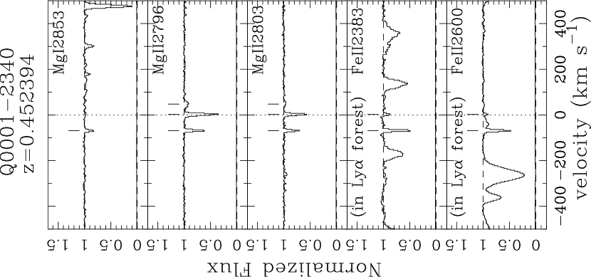
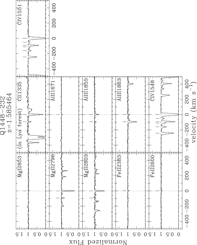
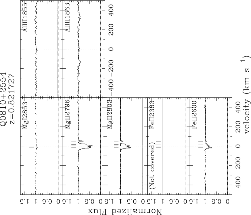
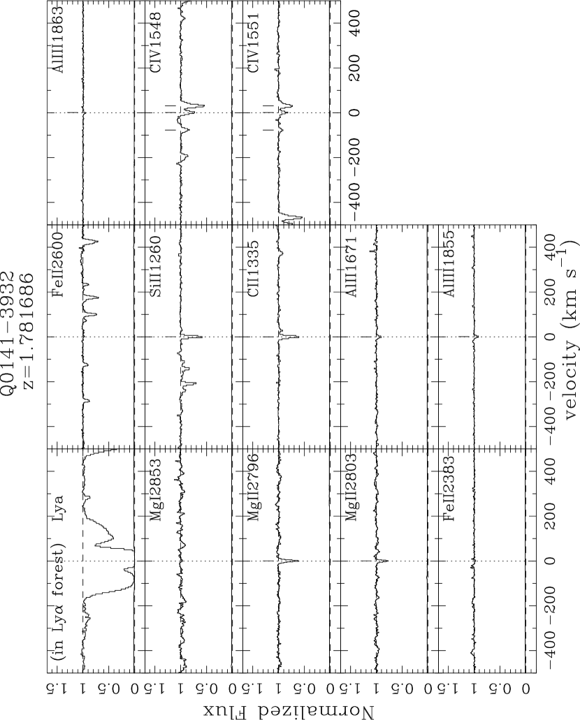
Figure 1.— A few example systems plots from the $100$ weak Mg ii absorbers in our sample represented on a velocity scale with the system redshift corresponding to $0$ km s^-1. The vertical axis is continuum normalized scale for the spectra. The vertical tick marks correspond to the centroid of the absorption components in each spectral feature, derived from Voigt profile fitting. Regions that are blueward of the Ly-$\alpha$ emission of the quasar are labeled in the respective panels as in Ly-$\alpha$ forest. The quasar name and redshift of the system are also labeled in each system plot. (Note: The full set of system plots will be presented in the online version of the journal.)

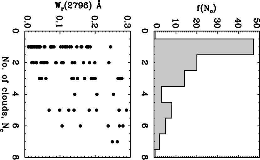
Figure 2.— The top panel shows the frequency distribution of the number of weak Mg ii clouds (i.e. number of Voigt profile components) in our sample. Single cloud systems account for 48% of the total number of systems.The bottom panel compares the rest-frame integrated equivalent width of $\hbox{{\rm Mg~{}}\kern 1.00006pt{\sc ii}}\lambda 2796$ line as a function of the number of clouds. Most of the weaker systems [$W_{r}(2796)<0.1$ Å] have absorption only in one or two clouds.

Figure 3.— Distribution of single and multiple cloud weak Mg ii systems as a function of redshift. The redshift distribution is comparable between the two types of systems (N${}_{c}=1$ and N${}_{c}\geq 2$; i.e., single and multiple cloud) and they do not exhibit preference for either low ($z\sim 1$) or high ($z\sim 2$) redshift.

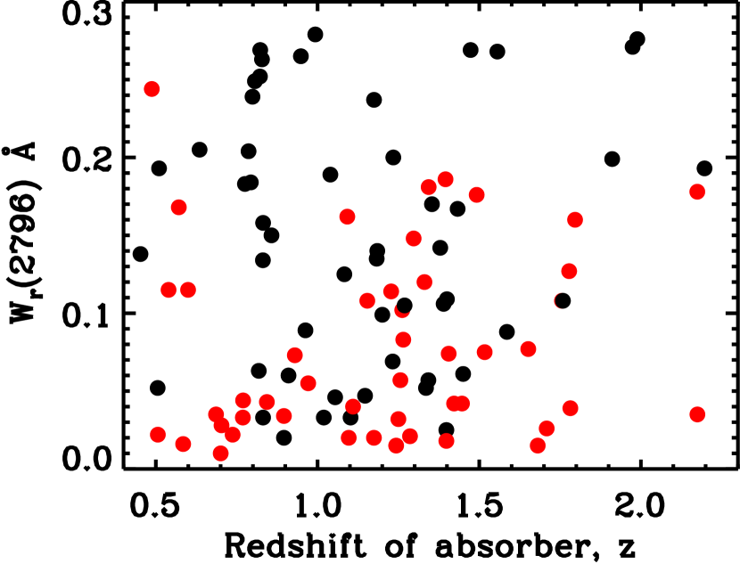
Figure 4.— The total (i.e. integrated) rest-frame equivalent width of $\hbox{{\rm Mg~{}}\kern 1.00006pt{\sc ii}}\lambda 2796$ Å in each absorber, as a function of the absorber’s redshift. The red and black data points correspond to single and multiple cloud systems respectively. It is evident that there is no significant correlation between the strength of weak absorber and its redshift.

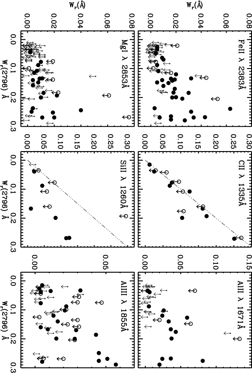
Figure 5.— The comparison of the total rest-frame equivalent widths of Mg ii ($W_{r}(2796)$) in each absorber, with other corresponding low ionization transitions and Al iii. The large solid dots are 3$\sigma$ detections, the large open circles are detections that are affected by blending with an absorption feature at some other redshift, in which case the measurement is considered as an upper limit, indicated by a downward pointing arrow from the open circle. Non-detections at the 3$\sigma$ level are plotted using just the downward pointing arrow. In most cases, the blending was from H i lines of the Ly-$\alpha$ forest. The equivalent width corresponding to non-detections at the 3$\sigma$ level are plotted using downward pointing arrows. The dash-dot line in the C ii and Si ii panels are the $y=x$ line for comparison with Mg ii. The correlation coefficients (Spearman’s $\rho$) between $W_{r}(\hbox{{\rm Mg~{}}\kern 1.00006pt{\sc ii}})$ and $W_{r}(\hbox{{\rm Fe~{}}\kern 1.00006pt{\sc ii}})$, $W_{r}(\hbox{{\rm Mg~{}}\kern 1.00006pt{\sc i}})$, $W_{r}(\hbox{{\rm C~{}}\kern 1.00006pt{\sc ii}})$, $W_{r}(\hbox{{\rm Si~{}}\kern 1.00006pt{\sc ii}})$, $W_{r}(\hbox{{\rm Al~{}}\kern 1.00006pt{\sc ii}})$, $W_{r}(\hbox{{\rm Al~{}}\kern 1.00006pt{\sc iii}})$ are 0.64(0.00), 0.50(0.00), 0.75(0.00), 0.38(0.20), 0.67(0.00), and 0.38(0.00) respectively. The value in parentheses represents the significance level, i.e., the probability that the observed value of $\rho$ would be greater than or equal to the actual value by chance.

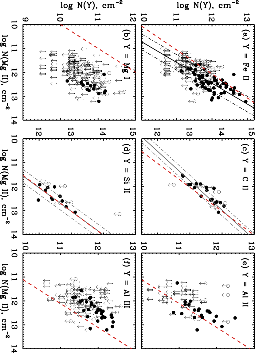
Figure 6.— The comparison of Mg ii column densities with the column density of other low ionization transitions and Al iii. The large solid dots are 3$\sigma$ detections, the large open circles are detections that are affected by blending with an absorption feature at some other redshift, in which case the measurement is considered as an upper limit, indicated by a downward pointing arrow from the open circle. The column density of non-detections, estimated from the $3\sigma$ equivalent width limit, are plotted using just the downward pointing arrows. The solid line is a linear regression fit formalizing the relationship between the two ions. The standard deviation of the corresponding fits are indicated by the dashed-dot line. The regression lines are drawn for the three ions (Fe ii, C ii and Si ii) that display the least scatter with N(Mg ii). The red dashed line in each panel indicates the solar abundance pattern based on values given in Grevesse & Sauval (1998); Allende Prieto et al. (2001, 2002) and Holweger et al. (2001). In the lower left panel, the red dashed line therefore corresponds to $y=x$.

Figure 7.— Cloudy photoionization curves indicating how the column density of Si ii, C ii, Mg ii, Fe ii, Al ii and Mg i change with ionization parameter (log $U$), metallicity ($Z$) and neutral hydrogen column density [$N(\hbox{{\rm H~{}}\kern 1.00006pt{\sc i}})$]. The density ($n_{\hbox{{\rm H}}}$) was calculated using the expression log $n_{\hbox{{\rm H}}}$ = log $n_{\gamma}$ - log $U$, for log $n_{\gamma}$ = -4.70, corresponding to the number density of ionizing photons ($h\nu\geq 13.6$ eV) at $z=2$.

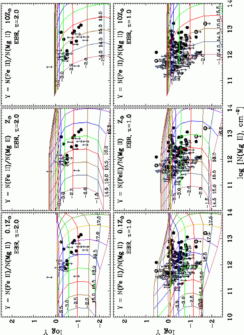
Figure 8.— Cloudy grid of photoionization models for 0.1Z_⊙, Z_⊙ and 10Z_⊙ metallicity with measurements of Fe ii and Mg ii column density over-plotted. Vertical curves correspond to lines of constant $N(\hbox{{\rm H~{}}\kern 1.00006pt{\sc i}})$ and the horizontal curves lines of constant ionization parameter (log $U$). The Cloudy models were computed for the intensity of the extragalactic ionizing background radiation (EBR) at $z=2$ and $z=1$. Weak Mg ii clouds at $z\geq 1.5$ are plotted in the EBR at $z=2$ panel and clouds at $z<1.5$ are plotted in the EBR at $z=1$ panel. The large solid dots are 3$\sigma$ detections, the large open circles are detections that are affected by blending with an absorption feature at some other redshift, in which case the measurement is considered as an upper limit, indicated by a downward pointing arrow from the open circle. The column density of non-detections, estimated from the $3\sigma$ equivalent width limit, are plotted using just the downward pointing arrows.

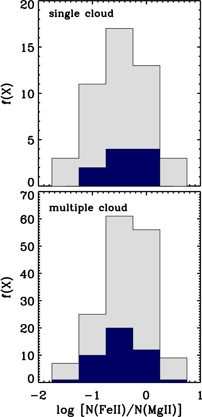
Figure 9.— The distribution of Fe ii to Mg ii column density ratio for single and multiple cloud systems. The histogram filled with the light color includes measurements that are upper limits in Fe ii, whereas the histogram filled with the dark color excludes those. For multiple clouds, we have included the Fe ii to Mg ii ratio in individual clouds. It is evident from the figure that both single and multiple cloud systems span roughly the same range of Fe ii to Mg ii column density ratios.

Figure 10.— Cloudy grid of photoionization models with measurements of Mg i and Mg ii column density over-plotted. The description of the Cloudy curves and the data points are the same as in Figure 8.

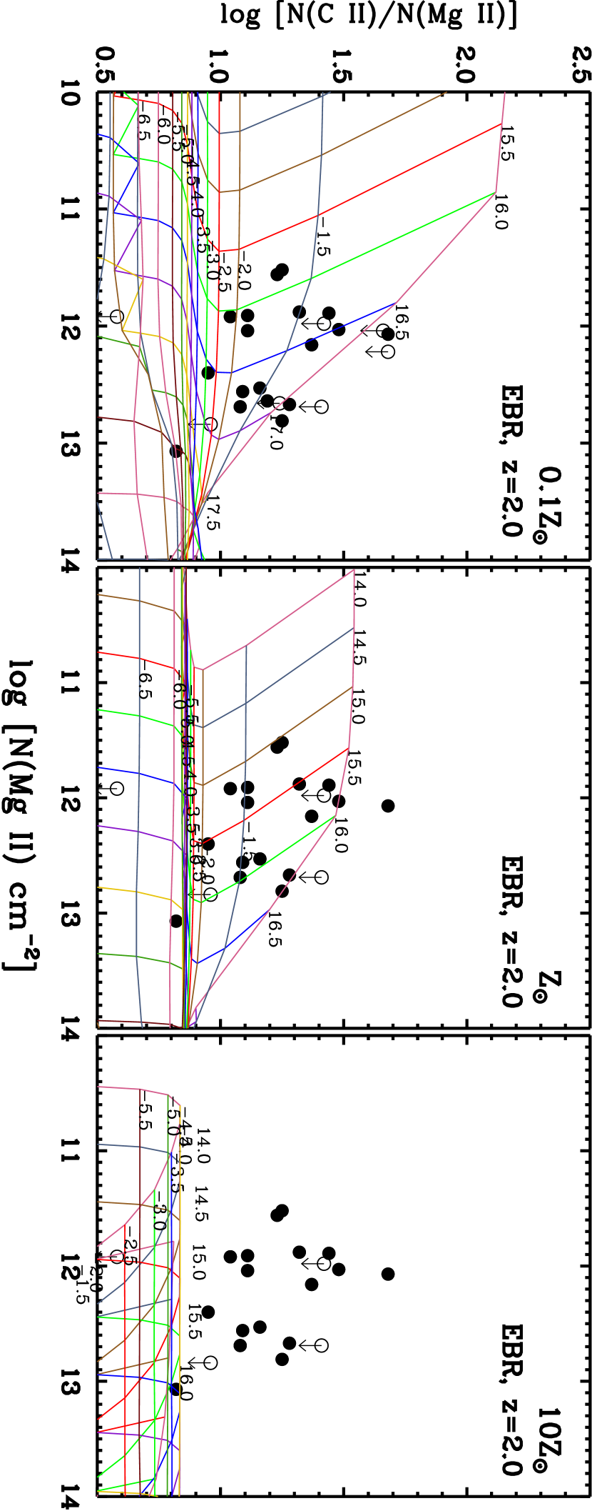
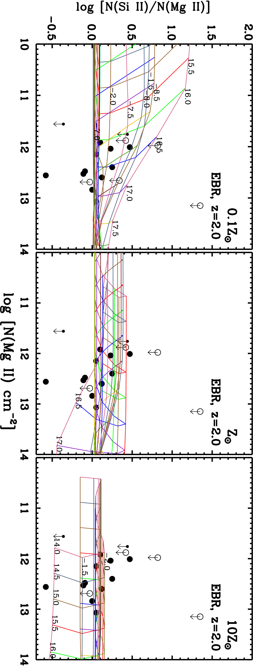
Figure 11.— Cloudy grid of photoionization models with measurements of C ii and Mg ii column density over-plotted. The description of the Cloudy curves and the data points are the same as in Figure 8. Almost all weak Mg ii absorbers with coverage of $\hbox{{\rm C~{}}\kern 1.00006pt{\sc ii}}\lambda 1335$ are at $z\geq 1.5$ and therefore we plot all of them on the $z=2$ EBR plot.

Figure 12.— Cloudy grid of photoionization models with measurements of Si ii and Mg ii column density over-plotted. The description of the Cloudy curves and the data points are the same as in Figure 8. Almost all weak Mg ii clouds with coverage of $\hbox{{\rm Si~{}}\kern 1.00006pt{\sc ii}}\lambda 1260$ are at $z\geq 1.5$ and therefore we plot all of them on the $z=2$ EBR plot.

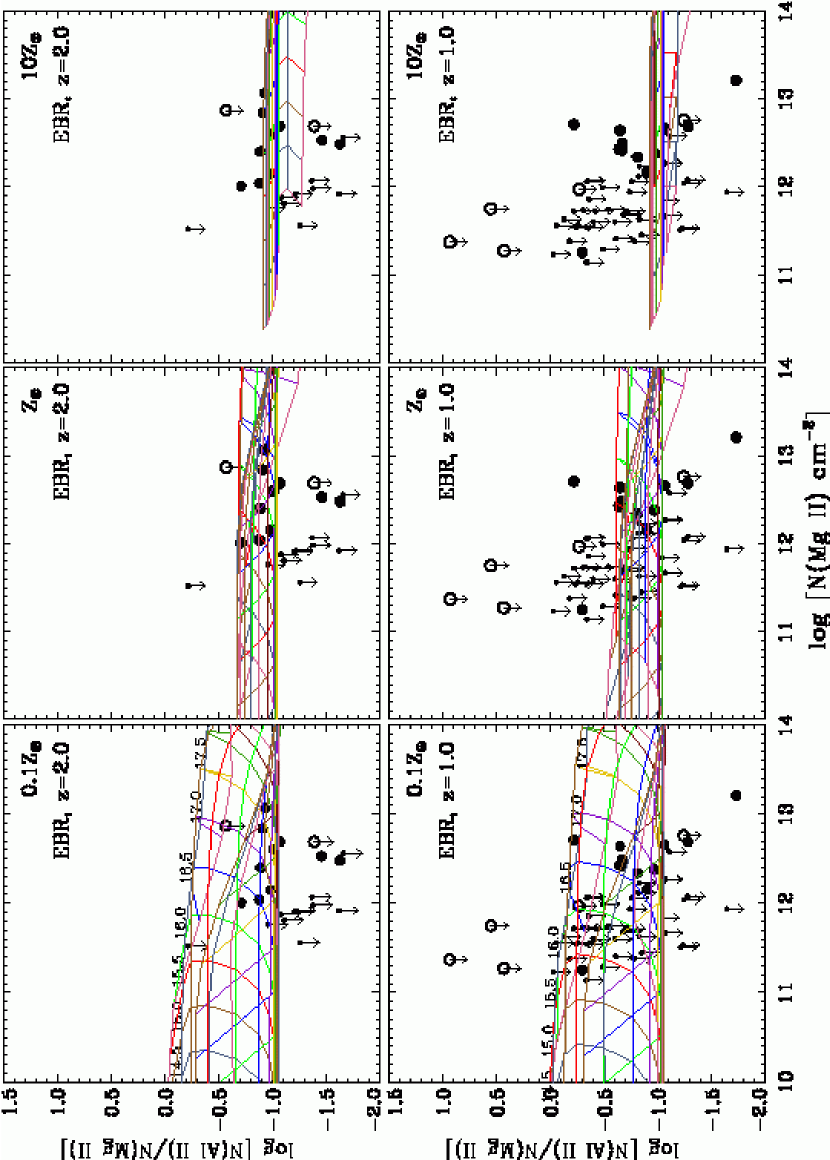
Figure 13.— Cloudy grid of photoionization models with measurements of Al ii and Mg ii column density over-plotted. The description of the Cloudy curves and the data points are the same as in Figure 8.

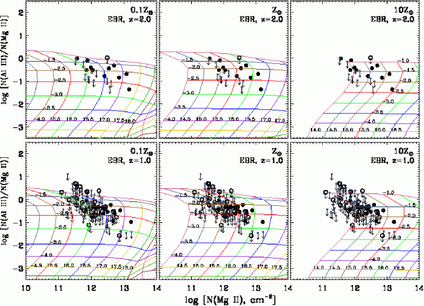
Figure 14.— Cloudy grid of photoionization models with measurements of Al iii and Mg ii column density over-plotted. The description of the Cloudy curves and the data points are the same as in Figure 8.

Figure 15.— Left Panel : The figure compares the C ii to Mg ii ratio with Fe ii to Mg ii in weak Mg ii clouds that have measurements for both C ii and Fe ii. The filled circles correspond to weak Mg ii clouds that had firm measurements for both C ii and Fe ii. The open circles correspond to data points in which either C ii or Fe ii or both have measurements that are upper limits. Middle Panel : compares the Al iii to Mg ii ratio with Al ii to Mg ii in weak Mg ii clouds that have measurements for both Al iii and Al ii. Right Panel : compares the C ii to Mg ii ratio with Si ii to Mg ii in weak Mg ii clouds that have simultaneous measurements for both C ii and Si ii.

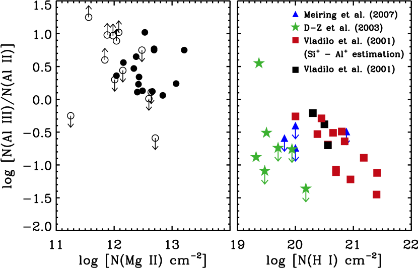
Figure 16.— On the left panel is the Al iii to Al ii ratio in weak Mg ii clouds discussed in this paper. Measurements that are upper limits in Al iii and Al ii are indicated using downward and upward pointing arrows respectively. The right panel shows the Al iii to Al ii ratio in sub-DLA and DLA systems taken from the literature. If weak Mg ii clouds are optically thin in H i (i.e. $N(\hbox{{\rm H~{}}\kern 1.00006pt{\sc i}})<10^{17}$ cm^-2), then the measurements indicate that the anti-correlation between $N(\hbox{{\rm H~{}}\kern 1.00006pt{\sc i}})$ and Al iii to Al ii ratio that is observed for DLA and sub-DLA systems, also extends to lower $N(\hbox{{\rm H~{}}\kern 1.00006pt{\sc i}})$ values.

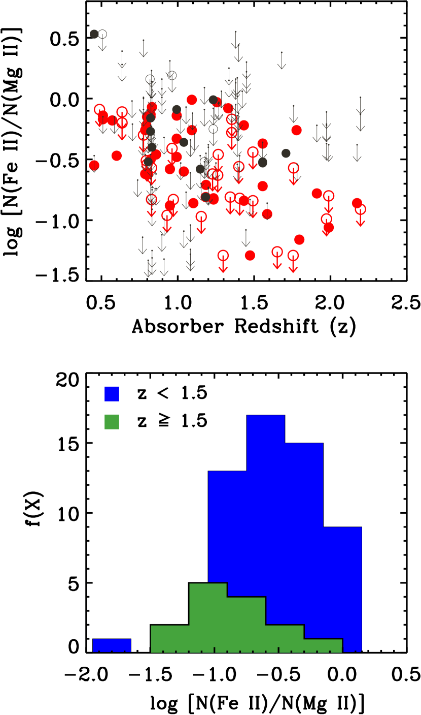
Figure 17.— Top panel : shows the Fe ii to Mg ii ratio in all the weak Mg ii clouds as a function of redshift of the system. The filled circles are firm detections (i.e. detections that are not limits), the large open circles with arrow pointing downward corresponds to Fe ii lines that are affected by blending with an absorption feature at some other redshift, in which case the measurement is considered as an upper limit. The non- detections at the $3\sigma$ level are plotted using downward pointing arrows. Those weak Mg ii clouds in which $N(\hbox{{\rm Mg~{}}\kern 1.00006pt{\sc ii}})>10^{12.2}$ cm^-2 are plotted in red. Bottom panel : shows the distribution of Fe ii to Mg ii in absorbers at $z\geq 1.5$ and $z<1.5$. The width of each bin in the distribution is 0.3. The data used to create the frequency distribution includes only those weak Mg ii clouds in which $N(\hbox{{\rm Mg~{}}\kern 1.00006pt{\sc ii}})>10^{12.2}$ cm^-2, below which a large fraction of systems only have upper limits for Fe ii.

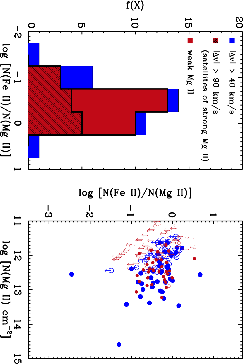
Figure 18.— The figure compares the column density ratio between Fe ii and Mg ii for weak Mg ii clouds and the high velocity components (i.e. satellite clouds) of strong Mg ii systems. In the right panel the downward pointing arrows indicate measurements that are upper limits in $N(\hbox{{\rm Fe~{}}\kern 1.00006pt{\sc ii}})$. The Fe ii and Mg ii column densities for the satellite clouds of strong Mg ii systems is taken from Churchill & Vogt (2001), and are represented as large blue points. The small red points correspond to weak Mg ii clouds presented in this paper. The left panel compares the distribution of the column density ratio between Fe ii and Mg ii for weak Mg ii clouds and the satellite clouds of strong Mg ii systems. The blue histogram is for the satellite clouds that are offset in velocity from the main absorbing component by $|\Delta v|>40$ km s^-1. The histogram shaded with lines is for the satellite clouds that are offset in velocity by $|\Delta v|>90$ km s^-1. The red histogram is the distribution for the sample of weak Mg ii clouds presented in this paper.

References

- Abraham et al. (1996) Abraham, R. G., van den Bergh, S., Glazebrook, K., Ellis, R. S., Santiago, B. X., Surma, P., & Griffiths, R. E. 1996, ApJS, 107, 1.
- Adelberger et al. (2005a) Adelberger, K. L., Shapley, A. E., Steidel, C. C., Pettini, M., Erb, D. K., & Reddy, N. A. 2005, ApJ, 629, 636.
- Adelberger et al. (2003) Adelberger, K. L., Steidel, C. C., Shapley, A. E., & Pettini, M. 2003, ApJ, 584, 45.
- Allende Prieto et al. (2001) Allende Prieto, C., Lambert, D. L., & Asplund, M. 2001, ApJ, 556, L63.
- Allende Prieto et al. (2002) Allende Prieto, C., Lambert, D. L., & Asplund, M. 2002, ApJ, 573, L137.
- Aracil et al. (2006) Aracil, B., Tripp, T. M., Bowen, D. V., Prochaska, J. X., Chen, H. -W., & Frye, B. L. 2006, MNRAS, 367. 139.
- Bauer et al. (2005) Bauer, A. E., Drory, N., Hill, G. J., & Feulner, G. 2005, ApJ, 621, 89.
- Bergeron et al. (1991) Bergeron, J., & Boissé, P. 1991, A&A, 243, 344.
- Bond et al. (2001) Bond, N. A., Churchill, C. W. C., Charlton, J. C., & Vogt, S. S. 2001, ApJ, 562, 641.
- Bouwens et al. (2003) Bouwens, R. J. et al. 2003, ApJ, 595, 589.
- Charlton et al. (2003) Charlton, J. C., Ding, J., Zonak, S. G., Churchill, C. W., Bond, N. A., & Rigby, J. R. 2003, ApJ, 589, 111.
- Charlton & Churchill (1998) Charlton, J. C., & Churchill, C. W. C. 1998, ApJ, 499, 181.
- Choi et al. (2006) Choi, P. I. et al. 2006, ApJ, 637, 227.
- Churchill (1997) Churchill, C. W. 1997, Ph.D. Thesis
- Churchill et al. (2007) Churchill, C. W. C., Kacprzak, G. G., Steidel, C. C., & Evans, J. L. 2007, ApJ, 661, 714.
- Churchill et al. (2005) Churchill, C. W. C., Kacprzak, G. G., Steidel, C. C. 2005, IAU Colloquium Proceedings, Cambridge University Press, pp 24-41.
- Churchill & Le Brun (1998) Churchill, C. W., & Le Brun, V. 1998, ApJ, 499, 677.
- Churchill et al. (1999) Churchill, C. W., Rigby, J. R., Charlton, J. C., & Vogt, S. S. 1999, ApJS, 120, 51.
- Churchill et al. (1996) Churchill, C. W., Steidel, C. C., & Vogt, S. S. 1996, ApJ, 471, 164.
- Churchill & Vogt (2001) Churchill, C. W., & Vogt, S. S. 2001, AJ, 122, 679.
- Churchill et al. (2003) Churchill, C. W. C., Vogt, S. S., & Charlton, J. C. 2003, ApJ, 125. 98
- Collins et al. (2004) Collins, J. A., Shull, J. M., & Giroux, M. L. 2004, ApJ, 605, 216
- Conselice et al. (2003) Conselice, C. J., Bershady, M. A., Dickinson, M., & Papovich, C. 2003, AJ, 126, 1183.
- Davé et al. (1997) Davé, R., Hernquist, L., Weinberg, D. H., & Katz, N. 1997, ApJ, 477, 21.
- Dekker et al. (2000) Dekker, H., D’Odorico, S., Kaufer, A., Delabre, B., & Kotzlowski, H. 2000, SPIE, 4008, 534.
- Dessauges-Zavadsky et al. (2003) Dessauges-Zavadsky, M., Péroux, C., Kim, T. S., D’Odorico, S., & McMahon, R. G. 2003, MNRAS, 345, 447.
- Ding et al. (2003) Ding, J., Charlton, J. C., Bond, N. A., Zonak, S. G., & Churchill, C. W. 2003, ApJ, 587, 551.
- Ellison et al. (2004) Ellison, S. L., Ibata, R., Pettini, M., Lewis, G. F., Aracil, B., Petitjean, P., & Srianand, R. 2004, A&A, 414, 79.
- Elmegreen et al. (2005) Elmegreen, D. M., Elmegreen, B. G., Rubin, D. S., & Schaffer, M. A. 2005, ApJ, 631, 85.
- Feigelson, & Nelson (1985) Feigelson, E. D., & Nelson, P. I. 1985, ApJ, 293, 192.
- Ferland et al. (1998) Ferland, G., Korista, K. T., Verner, D. A., Ferguson, J. W., Kingdon, J. B., & Verner, E. M. 1998, PASP, 110, 76.
- Fox et al. (2005) Fox, A. J., Wakker, B. P., Savage, B. D., Tripp, T. M., Sembach, K. R., & Bland-Hawthorn, J. 2005, ApJ, 630, 332
- Ganguly et al. (2005) Ganguly, R., Sembach, K. R., Tripp, T. M., & Savage, B. D. 2005, ApJS, 157, 251
- Grevesse & Sauval (1998) Grevesse, N., & Sauval, A. J. 1998, Space Science Reviews, 85, 161-174.
- Haardt & Madau (1996) Haardt, F., & Madau, P. 1996, ApJ, 461, 20.
- Heckman et al. (2000) Heckman, T. M., Lehnert, M. D., Strickland, D. K., & Armus, L. 2000, ApJS, 129, 493.
- Heckman et al. (2001) Heckman, T. M., Sembach, K. R., Meurer, G. R., Strickland, D. K., Martin, C. L., Clazetti, D., & Leitherer, C. 2001, ApJ, 554, 1021.
- Holweger et al. (2001) Holweger, H. 2001, Solar and Galactic Composition Workshop, Ed. by Robert F. Wimmer-Schweingruber. Pub. American Institute of Physics Conference Proceedings. Vol 598.
- Isobe et al. (1986) Isobe, T., Feigelson, E. D., & Nelson, P. I. 1986, ApJ, 306, 490.
- Kauffmann et al. (2004) Kauffmann, G., White, S. D. M., Heckman, T. M., Ménard, B., Brinchmann, J., Charlot, S., Tremonti, C., & Brinkmann, J. 2004, MNRAS, 353, 713.
- Keeney et al. (2006) Keeney, B. A., Stocke, J. T., Rosenberg, J. L., Tumlinson, J., & York, D. G. 2006, AJ, 132. 2496.
- Khare et al. (2005) Khare, P., et al. 2005, IAU Colloq. 199: Probing Galaxies through Quasar Absorption Lines, 427
- Kingdon et al. (1996) Kingdon, J. B., & Ferland, G. F. 1996, ApJS, 106, 205.
- Lanzetta et al. (1987) Lanzetta, K. M., Wolfe, A. M., & Turnshek, D. A. 1987, ApJ, 322, 739.
- Lavalley et al. (1992) Lavalley, M., Isobe, T., & Feigelson, E. 1992, 25, 245.
- Lynch et al. (2006) Lynch, R. S., Charlton, J. C., & Kim, T. -S. 2006, ApJ, 640, 81.
- Lynch & Charlton (2007) Lynch, R. S., & Charlton, J. C. 2007, ApJ, 666, 64.
- Masiero et al. (2005) Masiero, J. R., Charlton, J. C., Ding, J., Churchill, C. W., & Kacprzak, G. 2005, ApJ, 623, 57.
- Meiring et al. (2007) Meiring, J. D., Lauroesch, J. T., Kulkarni, V. P., Péroux, C., Khare, P., York, D. G., & Crotts, A. P. S. 2007, MNRAS, 376, 557.
- Milutinović et al. (2006) Milutinović, N., Rigby, J. R., Masiero, J. R., Lynch, R. S., Palma, C., & Charlton, J. C. 2006, ApJ, 641, 190.
- Misawa et al. (2007) Misawa, T., Charlton, J. C., & Narayanan, A. 2007, ApJ submitted.
- Mshar et al. (2007) Mshar, A. C., Charlton, J. C., Lynch, R. S., Churchill, C. W. C., & Kim, T. S. 2007, ApJ in press, arXiv0706.0515.
- Narayanan et al. (2005) Narayanan, A., Charlton, J. C., Masiero, J. R., & Lynch, R. 2005, ApJ, 632, 92.
- Narayanan et al. (2007) Narayanan, A., Misawa, T., Charlton, J. C., & Kim, T. S. 2007, ApJ, 660. 1093.
- Nestor et al. (2005) Nestor, D. B., Turnshek, D. A., & Rao, S. M. 2005, ApJ, 628, 637.
- Pettini et al. (2001) Pettini, M., Shapley, A. E., Steidel, C. C., Cuby, J. -G., Dickinson, M., Moorwood, A. F. M., Adelberger, K. L., & Giavalisco, M. 2001, ApJ, 554, 981.
- Putman et al. (2003) Putman, M. E., Bland-Hawthorn, J., Veilleux, S., Gibson, B. K., Freeman, K. C., & Maloney, P. R. 2003, ApJ, 597, 948
- Rauch et al. (1999) Rauch, M., Sargent, W. L. W., & Barlow, T. A. 1999, ApJ, 515, 500.
- Rauch et al. (2002) Rauch, M., Sargent, W. L. W., Barlow, T. A., & Simcoe, R. A. 2002, ApJ, 576, 45.
- Richter et al. (2008) Richter, P., Charlton, J. C., Fangano, A. P. M., Bekhti, N. B., & Masiero, J. R. 2008, ApJ submitted.
- Rigby et al. (2002) Rigby, J. R., Charlton, J. C., & Churchill, C. W. 2002, ApJ, 565, 743.
- Rupke et al. (2002) Rupke, D. S., Veilleux, S., & Sanders, D. B. 2002, ApJ, 570, 588.
- Sargent et al. (1989) Sargent, W. L. W., Steidel, C. C., & Boksenberg, A. 1989, ApJS, 69, 703.
- Schaye et al. (2007) Schaye, J., Carswell, R. F., & Kim, T. S. 2007, MNRAS, 379, 1169.
- Schwartz et al. (2006) Schwartz, C. M., Martin, C. L., Chandar, R., Leitherer, C., Heckman, T. M., & Oey, M. S. 2006, ApJ, 646, 858.
- Simcoe et al. (2004) Simcoe, R. A., Sargent, W. L. W., & Rauch, M. 2004, ApJ, 606, 92.
- Simcoe et al. (2006) Simcoe, R. A., Sargent, W. L. W., Rauch, M., & Becker, G. 2006, ApJ, 637, 648.
- Steidel et al. (1994) Steidel, C. C., Dickinson, M., & Persson, S. E. 1994, ApJ, 437, 75.
- Steidel et al. (2002) Steidel, C. C., Kollmeier, J. A., Shapley, A. E., Churchill, C. W., Dickinson, M., & Pettini, M. 2002, ApJ, 570, 526.
- Steidel & Sargent (1992) Steidel, C. C., & Sargent, W. L. W. 1992, ApJS, 80, 1.
- Stengler-Larrea et al. (1995) Stengler-Larrea et al. . 1995, ApJ, 444, 64.
- Stocke et al. (2004) Stocke, J. T., Keeney, B. A., McLin, K. M., Rosenberg, J. L., Weymann, R. J. & Giroux, M. L. 2004, ApJ, 609, 94.
- Tappe & Black (2004) Tappe, A. & Black, J. H. 2004, A&A, 423, 943.
- Timmes et al. (1995) Timmes, F. X., Woosley, S. E., & Weaver, T. A. 1995, ApJS, 98, 617.
- Tripp et al. (2006) Tripp, T. M., Aracil, B., Bowen, D. V., & Jenkins, E. B. 2006, ApJ, 643, 77.
- Tripp & Bowen (2005) Tripp, T. M., & Bowen, D. V. 2005, IAU Colloquium Proceedings, Cambridge University Press, pp 5-23.
- van den Bergh et al. (1996) van den Bergh, S., Abraham, R. G., Ellis, R. S., Tanvir, N. R., Santiago, B. X., & Glazebrook, K. G. 1996, AJ, 112, 359.
- Vladilo et al. (2001) Vladilo, G., Centurión, M., Bonifacio, P., & Howk, J. C. 2001, ApJ, 557, 1007.
- Wakker & van Woerden (1997) Wakker, B. P., & van Woerden, H. 1997, ARA&A, 35, 217
- Wang et al. (2006) Wang, W.-H., Cowie, L. L., & Barger, A. J. 2006, ApJ, 647, 74.
- York et al. (2006) York, D. G., et al. 2006, MNRAS, 367, 945
- Zonak et al. (2004) Zonak, S. G., Charlton, J. C., Ding, J., & Churchill, C. W. C. 2004, ApJ, 606, 196.