Numerical Simulation of Particle Flow in a Sand Trap

Abstract

Sand traps are used to measure Aeolian flux. Since they modify the surrounding wind velocity field their gauging represents an important challenge. We use numerical simulations under the assumption of homogeneous turbulence based on FLUENT to systematically study the flow field and trapping efficiency of one of the most common devices based on a hollow cylinder with two slits. In particular, we investigate the dependence on the wind speed, the Stokes number, the permeability of the membrane on the slit and the saltation height.

I Introduction

Dune motion, sand encroachment and desertification are based on sand transport by wind. Saltation is the basic mechanism of Aeolian sand flux Bagnold ; Owen ; Roux . The simplest and most common devices to measure it in the field are so called sand traps. They consist of cavities into which the sand bearing wind enters, drops the sand inside and then leaves again without the sand. In that way they accumulate inside the sand that would have crossed them during a given time, giving a measure for the flux through their cross section. The difficulty to quantitative gauge them arises in properly estimating this cross section because the trap being an extended fixed object modifies considerably the wind velocity field in its surrounding. The issue boils down to understand how much wind actually enters into the cavity and therefore strongly depends on the geometrical shape of the trap.

Among the many different trap designs that have been used in the past one of the simplest and most popular is a hollow cylinder with two slits, one open and the other covered by a membrane that is impermeable to the grains Maia see Fig. 1. It has been extensively implemented in field studies along the Northern coast of Brazil with much success. We will therefore study this particular device in detail by numerically solving the turbulent flow around an object having the corresponding geometry. We will calculate the trajectories of grains released at different positions in the area in front of the trap to assess if they are captured or not and do this for various Reynolds and Stokes numbers as well as different membrane permeabilities.

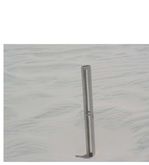
Figure 1: Cylindrical sand trap in use on a field dune.

This paper is organized as follows. In Section $2$, we introduce the model and briefly summarize the algorithm used in our simulation. In Section $3$ we present the qualitative and quantitative results. We conclude in Section $4$ by discussing the importance of these results in some practical applications.

II Model Formulation

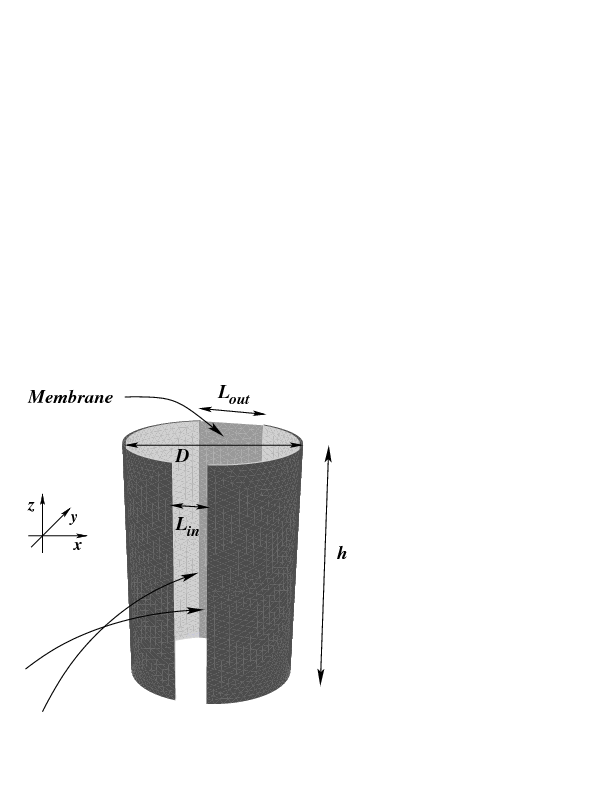
Figure 2: The geometry of the sand trap investigated here. $D$ is the diameter and $h$ the height. The widths of the vertical slits at the front and back sides are $L_{in}$ and $L_{out}$, respectively. Two possible grain trajectories are sketched.

As shown in Fig. 2 the sand trap that we study consists of a hollow cylinder of diameter $D$ and height $h$ closed on the top and the bottom, and having two vertical slits, one at the front and another at the back side. For simplicity we will neglect the width of the cylinder walls. A membrane covers the slit of the back side in order to capture particles with diameters larger than $0.01~{}mm$. The slits at the front and back sides have widths $L_{in}$ and $L_{out}$, respectively. We chose a height $h=1m$, a diameter $D=0.05m$ and slit widths $L_{in}=0.01m$ on the front side and $L_{out}=0.02m$ on the back side in agreement with typical dimensions of real devices. The membrane has a thickness of $\Delta m=0.001m$. Its permeability $\alpha$ can be modified and will be one of the control parameters of our simulation. In order to simulate the conditions of a realistic wind field we consider a box of size $1.5\times 1.5\times 1m$ with moving boundaries on top, left and right, i.e. in all directions transverse to the wind direction except for the bottom. On the fixed walls, i.e. the trap surface and the bottom we impose non-slip boundary conditions, which means that the velocity is equal to zero at the interfaces between solid and fluid. In order to reduce the size effects the simulation box was chosen to be one order of magnitude larger than diameter $D$ of the trap.

We assume that atmospheric air is an incompressible and Newtonian fluid having a viscosity of $\mu=1.7895\times 10^{-5}kg~{}m^{-1}~{}s^{-1}$ and a density of $\rho=1.225~{}kg/m^{3}$. The Reynolds number is defined as $Re\equiv\rho VL_{x}/\mu$, where $V$ is the average velocity and $L_{x}$ the linear size of the box in $x$ direction. This gives in our case $Re\approx 40000$ meaning that we can assume to be in a fully developed homogeneous turbulent state. The standard $k-\epsilon$ model is therefore an adequate way to solve the corresponding Reynolds-averaged Navier-Stokes equations of motion. Their numerical solution can be achieved by discretizing the velocity and pressure fields and using a control volume finite-difference technique Patankar ; Fluent . The convergence criteria of this scheme can be defined in terms of residuals, which measure up to which degree the conservation laws are satisfied. In our simulation we consider that convergence is achieved when each of the normalized residuals is smaller than $10^{-6}$.

A fully turbulent atmospheric boundary layer over a flat surface shows a logarithmic increase of the velocity $v(z)$ with the distance $z$ from the surface. Therefore, we impose a logarithmic velocity profile on the inlet, i.e. in the $x=0$ plane, of the form

$$v(z)=\frac{u_{*}}{\kappa}\ln\frac{z}{z_{0}},$$ (1)

where $u_{*}=0.36m/s$ denotes the shear velocity, $z_{0}=1.0\times 10^{-3}m$ the so called roughness length and $\kappa=0.4$ is the von Kármán constant Sauermann .

We model the fabric covering the opening at the backside of the trap as a special type of boundary condition mimicking a porous medium where the velocity/pressure drop characteristics are known. If $\Delta m$ is the thickness of this membrane then the pressure drop is defined according to Darcy’s law as:

$$\Delta p=-\frac{\mu}{\alpha}v\Delta m,$$ (2)

where $\alpha$ is the permeability of the medium and $v$ is the velocity normal to the membrane. In order to understand the effect of the membrane on the wind velocity field, we perform simulations using different membrane permeabilities, namely $\alpha=1.0\times 10^{-6}$, $1.0\times 10^{-8}$, $1.0\times 10^{-9}$ and $1.0\times 10^{-10}$.

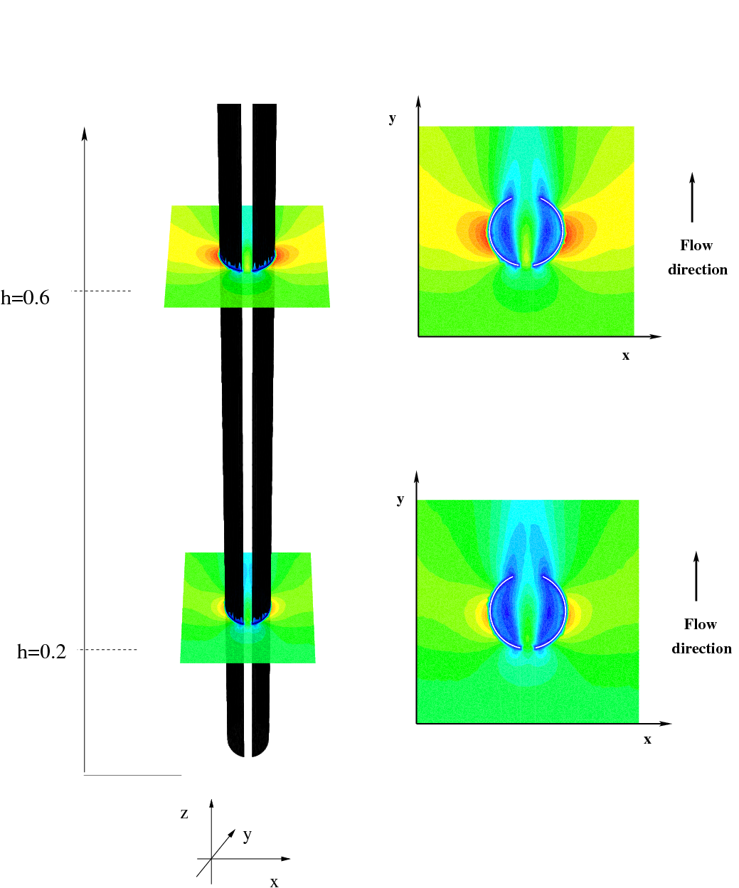
Figure 3: The pictures show the velocity profile in and around the sand trap. The images at right, show two different velocity profiles in a two dimensional cut (plane) through the sand trap at height $z=0.2$ and $z=0.6$. The wind velocity profile input at the surface $y=0$ comes form Eq. (1). The colors indicate the magnitude of the velocity varying from blue (low value) to red (high value). The picture corresponds to permeabilities $\alpha=1.0\times 10^{-6}$.

For simplicity we will only consider spherical particles. We also assume that the density of flying particles is so low that we can neglect collisions between them. For the same reason we will also neglect the momentum loss exerted by the particles on the fluid. Consequently the wind velocity and pressure fields can be calculated without knowing the particle positions and one can then obtain the trajectory of each particle by just integrating its equation of motion:

$$m_{p}\frac{d{\bf u}_{p}}{dt}=\sum{\bf F}_{p},$$ (3)

where $m_{p}$ and ${\bf u}_{p}$ are the mass and the velocity of a particle of diameter $d_{p}$ and $\sum{\bf F_{p}}$ is the total force acting on this particle. Let us assume that drag and gravity are the only relevant forces and that the particles do not interact with each other. Then the equation of motion for one particle can be rewritten as

$$\frac{d{\bf u}_{p}}{dt}=F_{D}({\bf u}-{\bf u}_{p})+{\bf g}\frac{(\rho_{p}-\rho)}{\rho_{p}},$$ (4)

where ${\bf g}$ is gravity acceleration and $\rho_{p}=2650~{}kg~{}m^{-3}$ is a typical value for the density of sand particles. The term $F_{D}({\bf u}-{\bf u}_{p})$ in Eq. (4) represents the drag force per unit particle-mass where

$$F_{D}=\frac{18\mu}{\rho_{p}d^{2}_{p}}\;\;\frac{C_{D}{\rm Re_{p}}}{24}.$$ (5)

Here $Re_{p}\equiv\rho d_{p}|{\bf u}-{\bf u}_{p}|/\mu$ is the particle Reynolds number and for the drag coefficient $C_{D}$ we use an empirical expression taken from Ref. Morsi . The trajectories of the particles are calculated by numerically integrating the equation of motion Eq. (4).

We characterize the effect of inertia on the air borne grains in the flow field through the dimensionless Stokes number $St$ which is defined by $St\equiv\rho_{p}{d_{p}}^{2}V/18L_{x}\mu$. For $St\gg 1$, inertia will dominate and the particles will move along straight lines not following the fluid, i.e. they will move in the air ballistically. For $St\ll 1$ particles behave as tracers and will perfectly follow the streamlines of the fluid. In our simulation we will vary the Stokes number by changing the particle diameter keeping all the other parameters constant. If a particle hits the outer surface of the sand trap it will be reflected elastically. If it hits the inner part of the trap it will stop moving, i.e. is counted as captured.

III Results and Discussions

We first present a study of the influence of the permeability $\alpha$ of the membrane on the fluid velocity field without the presence of particles. In order to understand essential features of the flow field around and inside the sand trap, we have performed extensive simulations by analyzing the flow for several values of permeability $\alpha$. To see the flow field we focus our attention on horizontal cuts through the trap, at a different distances $z=0.2$, and $z=0.6$ from the ground.

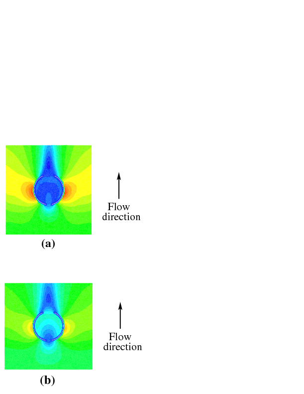
Figure 4: The pictures show the velocity profile in and around the sand trap. The images at right, show two different velocity profiles in a two dimensional cut through the sand trap at height $z=0.6$ $(a)$ and $z=0.2$ $(b)$. The wind velocity profile input comes from Eq. (1). The colors indicate the magnitude of the velocity varying from blue (low value) to red (high value). The picture correspond to permeabilities $\alpha=1.0\times 10^{-10}$.

Fig. 3 and Fig. 4 depict the velocity field around the sand trap for two different values of permeability, $\alpha=1.0\times 10^{-6}$ and $\alpha=1.0\times 10^{-10}$, respectively. Here we focus our discussion on the velocity profile, in the horizontal cuts through the trap at different heights $z$. We will first discuss the case of high permeability. In this case we can see in Fig. 3 that the wind velocity presents a parabolic profile in the channel inside the sand trap and also the existence of stagnation zones beside this channel.

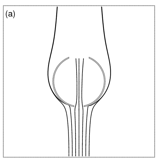
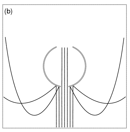
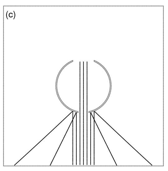
Figure 5: The $2D$ view of typical particles trajectories for three different Stokes numbers, $(a)$ $St=0.014$, $(b)$$St=1.43$ and $(c)$ $St=14.34$. The membrane permeability is $\alpha=1.0\times 10^{-6}$. The particles concentrate in the region of high velocities for all values of $St$.

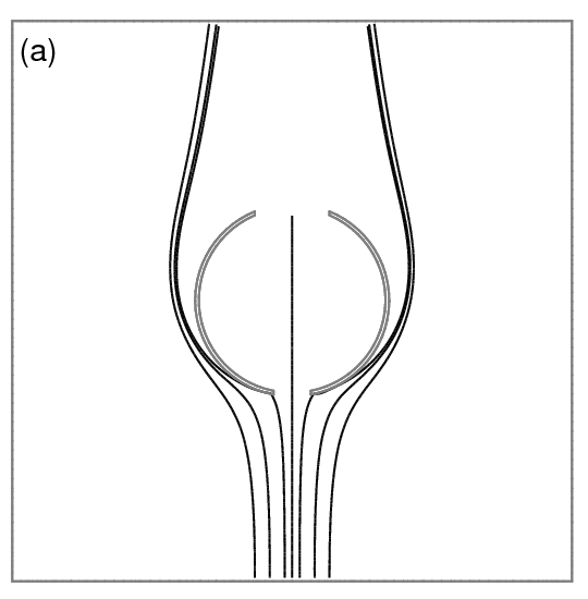
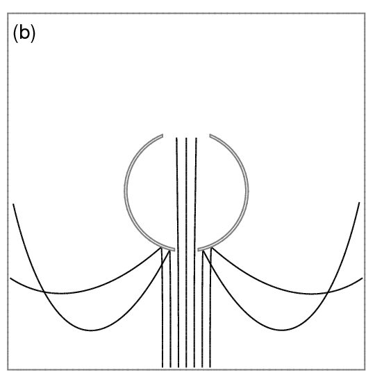
Figure 6: Typical particle trajectories projected on the $x-y)$ surface, for three different Stokes numbers, $St=0.014$ $St=1.43$ and $St=14.34$ correspond to $(a)$, $(b)$ and $(c)$, respectively. The value of the membrane permeability is $\alpha=1.0\times 10^{-10}$.

For low permeability, see Fig. 4, the velocity decreases along the center line to form a zone of low velocity close to the entrance of the sand trap while it increases around the trap. This increase of flow is due to the obstruction caused by the trap to the incompressible fluid. For larger heights $z$, the zone of low velocity reaches almost the entire region inside of the sand trap. With a decreasing membrane permeability also the formation of shadow zones can be observed behind the sand trap.

Our central issue is the study of sand transport and in particular the effect of the membrane permeability on the sand flux. Therefore we calculate particle trajectories by extensive simulations for different Stokes numbers and membrane permeabilities. In order to quantify the capture process the sand trap efficiency $\eta$ is defined as

$$\eta\equiv\frac{\phi}{\phi_{0}}$$ (6)

where $\phi_{0}$ is the total number of particles released during the interval $\Delta x$ and $\phi$ is the number of particles among these that have been captured. We will discuss in the following the efficiency $\eta$ as function of membrane permeability and Stokes number.

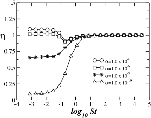
Figure 7: Semi-log plot of the efficiency $\eta$ of the sand trap as function of the Stokes number. The symbols correspond to different values of permeabilities $\alpha$, namely, (circles) $\alpha=1.0\times 10^{-6}$, (squares) $\alpha=1.0\times 10^{-8}$, (stars) $\alpha=1.0\times 10^{-9}$ and (triangles) $\alpha=1.0\times 10^{-10}$.

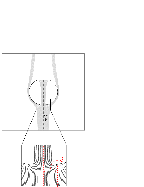
Figure 8: 2D view of typical particle trajectories for high permeability $\alpha=1.0\times 10^{-6}$ and low Stokes number $St=0.14$ at height $z=0.2$. The distance $\delta$ is the maximum distance from the symmetry line for which the particles bend towards the entrance of the sand trap. The stagnation zones are shown in more detail in the inset revealing how the particle trajectories can bend towards the symmetry line of the sand trap.

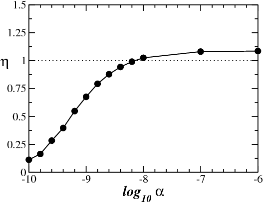
Figure 9: Semi-log plot of the efficiency $\eta$ as function of the membrane permeability $\alpha$, for fixed Stokes number $St=1.0\times 10^{-2}$. The doted line is included as guide to eye and corresponds to $\eta=1$.

Initially the grains are placed at $y=0$, a given height $z$ and randomly within the interval, $-0.01m<x<0.01m$. For a fixed value of $St$ and $\alpha$, we release up to $1000$ particles to determine the efficiency of the sand trap. We show in Figs. 5 and 6 the trajectories of $7$ particles for two different permeabilities, $\alpha=1.0\times 10^{-6}$ and $\alpha=1.0\times 10^{-10}$, respectively, and different Stokes numbers. For both figures the Stokes numbers are from top to bottom: $St=0.014$, $St=1.43$ and $St=14.34$. In the case of high permeability, as shown in Fig. 5, the grains concentrate in the regions of large velocities. Inside of the trap the particle trajectories do spread apart more with decreasing Stokes number. This effect is more pronounced at lower permeability. For high Stokes numbers some particles collide with the trap surface revers their direction and leave the box simulation. For intermediate Stokes numbers these particles also collide but are then deviated by the wind flow. This effect is independent of the permeability.

The dependence of the sand trap efficiency $\eta$ on the Stokes number is shown in Fig. 7 for different values of $\alpha$. We performed simulations for membrane permeabilities $\alpha=1.0\times 10^{-6}$, $1.0\times 10^{-8}$, $1.0\times 10^{-9}$ and $1.0\times 10^{-10}$ at many different heights $z$, with an inlet velocity given by Eq. 1. The value of $\eta$ was obtained from the average over different heights $z$, where at each one we released $1000$ particles. We see that $\eta$ presents two different regimes as function of the permeability $\alpha$. Let us first discuss the case of low permeabilities. In the limit of small Stokes numbers the efficiency of the sand trap is small and remains essentially constant close to zero. Since $St\ll 1$ the particles can be considered as tracers that nearly exactly follow the streamlines of the flow, avoiding trapping because practically no streamline crosses the interior of the trap as consequence of the low membrane permeability. Indeed we observe in these cases stagnation zones inside the sand trap. Above $St\approx 0.05$ the efficiency $\eta$ increases as function of the Stokes number. For high values of $St$ the efficiency reaches a saturation value close to unity. In this limiting case the particles move ballistically towards the sand trap and those that have been released within the range $-0.005m<x<0.005m$ are captured.

For high permeabilities $\alpha$, the efficiency $\eta$ presents an unexpected behavior in the region of low $St$, as shown in Fig. 7. For large Stokes numbers the efficiency $\eta$ remains constant until $St\approx 10.0$. Below this value surprisingly we detect a small minimum followed by an increase to a value that can be above one. We can explain this behavior observing the particle trajectories in the region close to the entrance of the sand trap as shown in Fig. 8.

For small membrane permeability the sand trap behaves like a solid cylinder. In this case a stagnation region appears in front of the trap around the symmetry line. As the permeability $\alpha$ increases some air can cross the sand trap and two stagnation zones appear beside the entrance and outside of the trap. Each of them has a separation point and all particle trajectories between these two separation points bend towards the center and enter the trap as confirmed in the simulation for low Stokes number as shown in Fig. 8. Therefore the number of captured particles and the efficiency of the sand trap can increase beyond the ballistic case.

For a fixed value of $St$ and different permeabilities $\alpha$, we search the maximum distance from the symmetry line $\delta$ at which the particles bend towards the entrance of the sand trap. This $\delta$ can be used as a measure for the increase in the sand trap efficiency. In Fig. 9, we show in a semi-log plot the efficiency $\eta$, which has been calculated from the parameter $\delta$, against the membrane permeability $\alpha$. Clearly, the curves display a strong change starting at the permeability $\alpha=1.0\times 10^{-8}$. This is the smallest permeability which still affects the efficiency of the sand trap.

IV Conclusions

In this paper, we have studied numerically the behavior of a sand trap frequently used to measure aeolian sand transport in the field. We solved the turbulent wind velocity field in the presence of the sand trap and investigated the effect of the membrane permeability. We studied quantitatively the particle trajectories carried by the fluid for different membrane permeabilities.

We have shown how the efficiency of the sand trap depends on the Stokes number and gave some insight about the effect of the membrane permeability on the capturing process.

As previously observed the membrane permeability strongly influences the capture process at low Stokes numbers. The sand trap efficiency $\eta$ exhibits a surprising increase above one, for large permeabilities and small Stokes numbers. Let us point out that only at higher $St$ values, when the trajectories of the particles are completely ballistic, the efficiency $\eta$ becomes independent on the membrane permeability. This is a useful result since for natural sand, for example on dunes, the grain size is around $200\mu m$ which corresponds to a rather high Stokes number. Our results therefore confirm that this type of sand trap is adequate to measure aeolian sand flux. The area of the slit at the entrance essentially equals the cross section over which the sand flux is measured independently on the details of the membrane on the back side.

V Acknowledgments

We would like to thank André Moreira for helpful discussions. We acknowledge CNPq, CAPES, FINEP and FUNCAP/CNPq/PPP and the Max Planck prize for financial support.

References

- (1) L.P. Maia Procesos Costeros y Balance Sedimentario a lo largo de Fortaleza (NE Brazil): Implicaciones para una Gestión Adecuada de la Zona litoral (PhD thesis, Faculty of Geology, University of Barcelona) (1998).
- (2) R.A. Bagnold, The Physics of Blown Sand and Desert Dunes (Methuen, London, 1939).
- (3) P.R. Owen, “Saltation of uniform grains in air,” J. Fluid Mech. 20, 225-242 (1964).
- (4) J.P. Le Roux, “Grains in motion: A review,” Sedimentary Geology 178, 285-313 (2005).
- (5) S.V. Patankar, Numerical Heat Transfer and Fluid Flow (Hemisphere, Washington, DC, 1980).
- (6) The FLUENT (trademark of FLUENT Inc.) commercial package for fluid dynamics analysis is used in this calculation.
- (7) G. Sauermann, J.S. Andrade Jr., L.P. Maia, U.M.S. Costa, A.D. Araújo and H.J. Herrmann, “Wind velocity and sand transport on barchan dune,” Geomorphology 54, 245-255, (2003).
- (8) S.A. Morsi and A.J. Alexander, “An investigation of particle trajectories in two-phase flow systems,” J. Fluid Mech. 55, 193 (1972).
- (9) A.D. Araújo, J.S. Andrade, Jr., and H.J. Herrmann, “Critical role of gravity filters,” Phys.Rev. Lett. 97, 138001 (2006).