Berry Phase and the Breakdown of the Quantum to Classical Mapping for the Quantum Critical Point of the Bose-Fermi Kondo model

Abstract

The phase diagram of the Bose-Fermi Kondo model contains an SU(2)-invariant Kondo-screened phase separated by a continuous quantum phase transition from a Kondo-destroyed local moment phase. We analyze the effect of the Berry phase term of the spin path integral on the quantum critical properties of this quantum impurity model. For a range of the power-law exponent characterizing the spectral density of the dissipative bosonic bath, neglecting the influence of the Berry phase term makes the fixed point Gaussian. For the same range of the spectral density exponent, incorporating the Berry phase term leads instead to an interacting fixed point, for which a quantum to classical mapping breaks down. Some general implications of our results are discussed.

Quantum criticality has become a new paradigm in the study of the overall phase diagram of strongly correlated electron systems. Universal properties of a quantum critical point (QCP) are traditionally described in terms of a mapping to the classical critical fluctuations of an order parameter in elevated dimensions Sachdev (1999). The quantum to classical mapping is based on the notion that slow fluctuations of the order parameter are the only critical degrees of freedom. This notion has been challenged in a number of contexts. In the heavy fermion metals, an anti-ferromagnetic QCP can accommodate new quantum modes, which are characterized by a critical destruction of the Kondo effect Si et al. (2001); Coleman et al. (2001); v. Löhneysen et al. (2007); Gegenwart et al. (2008).

In addition to lattice Kondo systems, the critical Kondo destruction has also been studied in the Bose-Fermi Kondo model (BFKM) Zhu and Si (2002); Zaránd and Demler (2002). The first indication for the violation of the quantum to classical mapping came from a study in a dynamical large-$N$ limit of the spin-isotropic BFKM Zhu et al. (2004). For the spectral density of the bosonic bath of the form $|\omega|^{1-\epsilon}\text{sgn}\omega$, the large-$N$ limit yields an interacting fixed point not only for $0<\epsilon<1/2$ but also for $1/2\leq\epsilon<1$. Related conclusions were drawn based on the numerical renormalization group (NRG) studies of the related quantum impurity models with Ising anisotropy Vojta et al. (2005); Glossop and Ingersent (2005). Very recently, the results of the Ising anisotropic models have been the subject of renewed interest, in light of the contrasting behavior between the NRG results and those from Monte Carlo simulations of a classical Ising chain Kirchner and Si ; Winter et al. ; ? .

Given these recent developments, it is timely to address the issue of the quantum to classical mapping in the spin-isotropic BFKM. For this purpose, we consider the model in terms of a coherent-state spin path integral representation, which highlights the role of the Berry phase term. By separately considering the cases in the presence/absence of the Berry phase term, we establish that the breakdown of the quantum to classical mapping originates from the interference effect of the Berry phase term.

The spin-isotropic Bose-Fermi Kondo model:   The model is specified by the Hamiltonian,

$${\cal H}_{\text{\small bfkm}} = j_{K}~{}{\bf S}\cdot{\bf s}_{c}+\sum_{p\sigma}E_{p}~{}c_{p\sigma}^{\dagger}~{}c_{p\sigma}$$ (1)

$$+ \;g_{0}\sum_{p}{\bm{S}}\cdot\left({\bm{\phi}}_{p}+{\bm{\phi}}_{-p}^{\;\dagger}\right)+\sum_{p}w_{p}\,{\bm{\phi}}_{p}^{\;\dagger}{\bm{\phi}}_{p}\;.$$

Here ${\bf S}$ is a spin-$1/2$ local moment, $j_{K}$ and $g_{0}$ are the Kondo coupling and the coupling constant to the bosonic bath respectively, $c_{p\sigma}^{\dagger}$ describes a fermionic bath with a constant density of states, $\sum_{p}\delta(\omega-E_{p})=N_{0}$, and ${\bm{\phi}}_{p}^{\;\dagger}$ is the bosonic bath with the spectral density:

$$\mbox{Im}\chi_{0}^{-1}(\omega)\, \equiv \,\sum_{p}[\delta(\omega-w_{p})-\delta(\omega+w_{p})]$$ (2)

$$\,\sim \,|\omega|^{1-\epsilon}\text{sgn}(\omega)\Theta(\omega_{c}-|\omega|).$$

The partition function of this model is

$${\mathcal{Z}}\, = \,\int{\mathcal{D}}[\bar{c}_{\sigma},c_{\sigma},{\bm{\bar{}}{\phi}},{\bm{\phi}},\vec{n}]\,\delta(|\vec{n}|^{2}-1)$$ (3)

$$~{}~{}~{}~{}~{}~{}~{}\exp[{-S(\bar{c}_{\sigma},c_{\sigma},{\bm{\bar{}}{\phi}},{\bm{\phi}},\vec{n})}],$$

where $c_{\sigma}$ is a Grassmann variable for the fermionic coherent state, while $\phi$ and $\vec{n}$ are c-numbers for the bosonic and spin coherent states respectively. The action is given by

$$S = \,is[\omega(\vec{n})]+\int_{0}^{\beta}d\tau\,\sum_{p}(\Sigma_{\sigma}\bar{c}_{p\sigma}\partial_{\tau}c_{p\sigma}+{\bm{\bar{}}{\phi}_{p}}\partial_{\tau}{\bm{\phi}}_{p})$$ (4)

$$+ \,\int_{0}^{\beta}d\tau\,H_{\mbox{\tiny bfkm}}(\bar{c},c,{\bm{\bar{}}{\phi}},{\bm{\phi}},s\vec{n}).$$

Berry phase of the coherent-state spin path integral:   Eq. (4) is written in terms of the spin (or SU(2)) coherent states Perelomov (1986); Inomata et al. (1992). Just like bosonic coherent states, spin coherent states are generated by a unitary operator

$$|\xi>=T(\xi)|0>;~{}T(\xi)=e^{[\xi J^{\dagger}-\bar{\xi}J^{-}]}$$ (5)

acting on a suitably defined vacuum $|0>$ footnote . $J^{\dagger}$/$J^{-}$ is the raising/lowering operator of the spin algebra. and $\xi$ is a c-number. Alternatively, the coherent state can be represented as a point on the three-dimensional unit sphere, $\vec{n}$, which is parameterized by the two angles $\Theta$ and $\phi$; $\xi=(1/2)\Theta e^{i\phi}$.

In Eq. (4), the path integral runs over all periodic paths, i.e. $\vec{n}(0)=\vec{n}(\beta)$. $\omega(\vec{n})$ is a geometrical phase and equals the area on the unit sphere enclosed by $\vec{n}(\tau)$. $s$ is the spin of the local moment. In the following, we will be considering the appropriate SU(N) or O(N) generalizations of the SU(2) model.

Model in the absence of the Berry phase:   We consider first the quantum critical properties of the BFKM without the Berry phase term. Simply removing the Berry phase term from the functional integral, Eq. (4), results in an ill-defined measure. Restraining however the spin path integral to a subset of paths with identical Berry phase, e.g. the subset of all great circles, the Berry phase term can be absorbed into the normalization of the partition function. After integrating out the bosonic bath, this leads to

$${\mathcal{L}}\, = \,i\mu(\tau)[\sum_{i}^{3}n_{i}^{2}-1]+J_{K}\vec{n}(\tau)\cdot\bar{c}(\tau)\vec{\sigma}c(\tau)$$

$$+ \,\sum_{\sigma}\int_{0}^{\beta}d\tau^{{}^{\prime}}\bar{c}_{\sigma}(\tau)G_{c}^{-1}(\tau-\tau^{{}^{\prime}})c_{\sigma}(\tau^{{}^{\prime}})$$

$$+ \,g^{2}\int_{0}^{\beta}d\tau^{{}^{\prime}}\vec{n}(\tau)G_{\phi}(\tau-\tau^{{}^{\prime}})\vec{n}(\tau^{{}^{\prime}}),$$ (6)

with $i\mu(\tau)$ being a Lagrangian multiplier enforcing the constraint $\sum_{i}^{3}n_{i}^{2}=1$, $J_{K}=sj_{K}/2$, and $g=sg_{0}$. $G_{c}=-\langle T_{\tau}c_{\sigma\alpha}(\tau)c_{\sigma\alpha}^{\dagger}(0)\rangle_{0}$, and ${\cal G}_{\phi}=\langle T_{\tau}\phi(\tau)\phi^{\dagger}(0)\rangle_{0}$. The terms involving the electron fields are quadratic in them, so the electron fields can be exactly integrated out as well:

$${\mathcal{Z}}\, = \,\int{\mathcal{D}}[\vec{n}]\,Det\Big{[}G_{c}^{-1}(\tau-\tau^{{}^{\prime}})\delta_{\sigma\sigma^{{}^{\prime}}}\!+\!J_{K}\vec{n}(\tau)\cdot\vec{\sigma}\delta(\tau-\tau^{{}^{\prime}})\Big{]}$$ (7)

$$\times\exp[-\int_{0}^{\beta}d\tau i\mu(\tau)[\sum_{i}^{3}n_{i}^{2}(\tau)-1]$$

$$+g^{2}\int_{0}^{\beta}d\tau\int_{0}^{\beta}d\tau^{{}^{\prime}}\vec{n}(\tau)G_{\phi}(\tau-\tau^{{}^{\prime}})\vec{n}(\tau^{{}^{\prime}})].$$

With the help of $\exp[\ln DetM]=\exp[Tr\ln M]$ the effective action can be expressed as

$$S\, = \,\int_{0}^{\beta}d\tau\,i\mu(\tau)[\sum_{i}^{3}n_{i}^{2}-1]$$

$$+ \,g^{2}\int_{0}^{\beta}d\tau\int_{0}^{\beta}d\tau^{{}^{\prime}}\vec{n}(\tau)G_{\phi}(\tau-\tau^{{}^{\prime}})\vec{n}(\tau^{{}^{\prime}})$$

$$+ \,Tr\ln(-G_{c}^{-1}\delta_{s,s^{{}^{\prime}}})$$

$$+ \,Tr\ln[{\bm{1}}-J_{K}G_{c}\vec{n}(\tau)\cdot\vec{\sigma}_{s,s^{{}^{\prime}}}\delta(\tau-\tau^{{}^{\prime}})].$$ (8)

The logarithm can be expanded in powers of $J_{K}G_{c}\vec{n}(\tau)\cdot\vec{\sigma}_{s,s^{{}^{\prime}}}\delta(\tau-\tau^{{}^{\prime}})$. The odd powers in this expansion vanish, since the Pauli matrices are traceless.

In order to systematically study this action, we will first generalize it in such a way that the fluctuations around a saddle point vanish. To do so, we extend the O(3) invariance of the action to an $O(N^{2}-1)$ symmetry, with $\vec{n}$ containing $M\equiv N^{2}-1$ components. This corresponds to a generalization of Eq. (6) to the case with an $O(N^{2}-1)\times SU(N)$ symmetry. We rescale the coupling constants $J_{K}$ and $g$ in terms of N, so that a non-trivial large-N limit ensues. The required rescaling of $J_{K}$ is determined by the N-dependence of the quadratic term in the expansion of the logarithm of Eq. (8). $Tr(J_{K}\vec{n}\cdot\vec{A}\,G_{c})^{2}=Tr(J_{K}\sum_{i=1}^{N^{2}-1}n_{i}{\bm{A}}^{i}\,G_{c})^{2}$, where the trace is over the (extended) spin space. The ${\bm{A}}^{i}$ are Hermitean $N\times N$ matrices of unit determinant. We make use of the invariance of the trace and expand the generators in terms of N$\times$N matrices ${\bm{B}}^{l}$ ($l=1,\cdots,N^{2}$): ${\bm{A}}^{i}=\sum_{i}^{N^{2}}a_{i,l}{\bm{B}}^{l}$. The set ${\bm{B}}^{l}$ is chosen such, that the $l$th matrix ${\bm{B}}^{l}$ has ${\bm{B}}^{l}|_{s,t}=e^{i\phi}$ and ${\bm{B}}^{l}|_{t,s}=e^{-i\phi}$ if and only if $l=N(s-1)+t$ with $s=1,\ldots,N$ and $t=1,\ldots,N$. All other elements of ${\bm{B}}^{l}$ vanish identically. The particular value of $\phi$ is left unspecified since it will only affect the expansion coefficients $a_{i,l}$. $G_{c}$ is diagonal in the spin space. Therefore, the quadratic term should scale as $N\cdot M$. Rescaling $J_{K}^{2}\rightarrow J_{K}^{2}/M=\tilde{J}_{K}^{2}$ renders the second term proportional to $N$. Rescaling $g\rightarrow g/N=\tilde{g}$ has the same effect on the similar term in the the effective action involving the bosonic bath. Finally, the constraint needs to be generalized to $\sum_{i}^{N}n_{i}^{2}=q_{0}N$.

Taking all these together, the large-N limit of the $O(N^{2}-1)\times SU(N)$ model leads to a saddle-point equation

$$\chi^{-1}_{\mbox{\tiny loc}}(\tau)\,=\,\mu_{0}+\tilde{J}_{K}^{2}G_{c,x}(\tau)G_{c,\tilde{y}}(-\tau)+\tilde{g}^{2}G_{\phi}(\tau).$$ (9)

At the saddle point, $i\mu(\tau)=\mu_{0}$ satisfies

$$\sum_{n}\chi_{\mbox{\tiny loc}}(i\omega_{n})=q_{0}.$$ (10)

The second term of the RHS of Eq. (9) is just the particle hole bubble of the conduction electrons, with $G^{c}_{x}(\tau)G^{c}_{\tilde{y}}(-\tau)\sim 1/\tau^{2}$. The long-time behavior of $G_{\phi}(\tau)$ is specified by Eq. (2), $G_{\phi}(\tau)\sim 1/\tau^{2-\epsilon}$. Solving the saddle point equation for a diverging $\chi_{\mbox{\tiny loc}}(\tau)$ results in a critical $\chi_{\mbox{\tiny loc}}$ with $\chi_{\mbox{\tiny loc}}(\tau)\sim 1/\tau^{\epsilon}$, implying

$$\chi_{\mbox{\tiny loc}}(\omega,T=0)\sim 1/(-i\omega)^{1-\epsilon}.$$ (11)

Away from the saddle point, i.e. for a finite $N$, additional interactions are present. The Lagrangian multiplier $\mu$ acquires a $\tau$ dependence, $i\mu(\tau)=\mu_{0}+\Delta\mu(\tau)/N$ to the sub-leading order. This generates a new interaction vertex of the form $\Delta\mu(\tau)n^{2}(\tau)/N$, which gives rise to a quartic coupling of the field $n(\tau)$:

$$\frac{u}{N}\prod_{i}^{4}\int d\omega_{i}\delta(\sum_{i}^{4}\omega_{i})\prod_{i}^{4}n(\omega_{i}).$$ (12)

The scaling dimension of the field $[n(\omega)]=(2-\epsilon)/2$ follows from Eq. (2). As a result, the scaling dimension of the quartic coupling is $[u]=2(\frac{1}{2}-\epsilon)$ Fisher et al. (1972). For $\epsilon<1/2$, $u$ is a relevant perturbation and the low-energy properties of the system will be governed by an interacting fixed point with $u^{*}\neq 0$ and consequently hyperscaling and $\omega/T$-scaling. This interacting fixed point is the Ginzburg-Wilson-Fisher fixed point of the local $\phi^{4}$-theory. For $1/2\leq\epsilon<1$, $u$ is irrelevant and will flow to zero; the Gaussian fixed point will be stable. A vanishing quartic coupling makes the approach to the fixed point singular; in other words, $u$ is dangerously irrelevant and therefore spoils hyperscaling and $\omega/T$-scaling. In the context of the long-ranged Ising model this process has been discussed recently in Kirchner and Si . The dangerously irrelevant coupling leads to

$$\chi_{\mbox{\tiny loc}}(\omega=0,T)\sim 1/T^{\frac{1}{2}}$$ (13)

Comparing Eqs. (11,13) shows that $\chi_{\mbox{\tiny loc}}(\omega,T)$ disobeys an $\omega/T$ scaling.

Model in the presence of the Berry phase:  

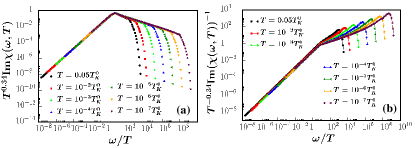
Figure 1: Scaling plot of (a) $T^{0.34}\mbox{Im}\chi_{\mbox{\tiny loc}}(\omega,T)$ and (b) $T^{-0.34}\mbox{Im}\big{(}1/\chi_{\mbox{\tiny loc}}(\omega,T)\big{)}$ for $\epsilon=2/3$. Numerical parameters are specified in the main text.

In order to generalize SU(2) to SU(N) within a path integral formulation it is necessary to use proper coherent states over SU(N). Such coherent states can be constructed in analogy to the SU(2) case and a corresponding Berry phase term for the SU(N) spin path integral with similar topological properties emerges Nemoto (2000); Mathur and Mani (2002); Read and Sachdev (1989). This model in the presence of the Berry phase term can be studied in a dynamical large-$N$ limit Zhu et al. (2004) of the SU(N)$\times$ SU($\kappa$ N) BFKM:

$${\cal H}_{\text{MBFK}} = ({J_{K}}/{N})\sum_{\alpha}{\bf S}\cdot{\bf s}_{\alpha}+\sum_{p,\alpha,\sigma}E_{p}~{}c_{p\alpha\sigma}^{\dagger}c_{p\alpha\sigma}$$ (14)

$$+ ({g}/{\sqrt{N}}){\bf S}\cdot{\bf\Phi}+\sum_{p}w_{p}\,{\bf\Phi}_{p}^{\;\dagger}\cdot{\bf\Phi}_{p},$$

where $\sigma=1,\ldots,N$ and $\alpha=1,\ldots,M$ are the spin and channel indices respectively, and ${\bf\Phi}\equiv\sum_{p}({\bf\Phi}_{p}+{\bf\Phi}_{-p}^{\;\dagger})$ contains $N^{2}-1$ components. The local moment is expressed in terms of pseudo-fermions $S_{\sigma,\sigma^{\prime}}=f^{\dagger}_{\sigma}f_{\sigma^{\prime}}-\delta_{\sigma,\sigma^{\prime}}Q/N$, where $Q$ is related to the chosen irreducible representation of SU(N) Parcollet and Georges (1998); Cox and Ruckenstein (1993). The quartic term between conduction electrons and pseudo-fermions is expressed in terms of a bosonic decoupling field $B_{\alpha}$. The large-$N$ saddle-point equations are

$$\Sigma_{B}(\tau) = -G_{c}(\tau)G_{f}(-\tau);$$

$$\Sigma_{f}(\tau) = \kappa G_{c}(\tau)G_{B}(\tau)+g^{2}G_{f}(\tau){\cal G}_{\Phi}(\tau);$$

$$G_{B}^{-1}(i\omega_{n}) = 1/{J_{K}}-\Sigma_{B}(i\omega_{n});$$

$$G_{f}^{-1}(i\omega_{n}) = i\omega_{n}-\lambda-\Sigma_{f}(i\omega_{n});$$ (15)

together with a constraint $G_{f}(\tau\rightarrow 0^{-})=Q/N$. Here, $\kappa=M/N$ and $\lambda$ is a Lagrangian multiplier. The analytically continued equations (15) can be self-consistently solved for any frequency ($\omega$) and temperature ($T$) Zhu et al. (2004). Eqs. (15) completely capture the (full) quantum dynamics of the problem and contain the effect of the Berry phase in the path integral approach. At the QCP, the order parameter susceptibility Zhu et al. (2004) behaves as

$$\chi_{\mbox{\tiny loc}}(\omega,T=0)\sim 1/\omega^{1-\epsilon};~{}~{}\chi_{\mbox{\tiny loc}}(\omega=0,T)\sim 1/T^{1-\epsilon}$$ (16)

for all $0<\epsilon<1$. Fig. 1(a) shows the the $\omega-T$-scaling of $\chi_{\mbox{\tiny loc}}(\omega,T)$ for $\epsilon=2/3>1/2$. The numerical parameters are $\kappa=1/2$, $Q/N=1/2$, and $N_{0}(\omega)=(1/\pi){\rm exp}(-\omega^{2}/\pi)$ for the conduction electron density of states. The nominal bare Kondo scale is $T_{K}^{0}N_{0}(0)\equiv{\rm exp}(-1/N_{0}(0)J_{K})\approx 0.06$, for fixed $J_{K}N_{0}(0)=0.8$. The bosonic bath spectral function $\sum_{p}\delta(\omega-w_{p})\sim\omega^{1-\epsilon}$ is cut off smoothly at $2\omega_{c}N_{0}(0)\approx 0.05$.

The $\omega/T$-scaling of $\chi_{\mbox{\tiny loc}}(\omega,T)$ for $1/2\leq\epsilon<1$ implies the breakdown of the quantum to classical mapping, since the mapped classical critical point does not obey $\omega/T$-scaling for this range of $\epsilon$. An important issue is whether the SU(N)$\times$ SU($\kappa$ N) result anchored around large N can be extended to a finite N or whether it is susceptible to the presence of dangerously irrelevant couplings. In order to address this question we introduce a self-energy for the order parameter susceptibility,

$$M(\omega,T)\equiv g_{c}^{2}\chi_{0}^{-1}(\omega)-1/\chi_{\mbox{\tiny loc}}(\omega,T),$$ (17)

where $\chi_{0}^{-1}(\omega)$ follows from Eq. (2) and $g^{2}_{c}(J_{K})$ is the value of the coupling constant $g^{2}$ at which the system becomes critical for a given $J_{K}$. The self-energy $M(\omega,T)$ thus defined will be $T$-dependent, since $\chi_{0}^{-1}(\omega)$ is $T$-independent but the inverse of $\chi_{\mbox{\tiny loc}}(\omega,T)$ shows non-trivial $\omega/T$-scaling, see Fig. 1(b). [By contrast, at the Gaussian fixed point arising in the case without the Berry phase term, described in the previous section, the corresponding self-energy $M(\omega,T)$ at $N=\infty$ is $T$-independent.] In Fig. 2(a) we show $\mbox{Im}(1/\chi_{\mbox{\tiny loc}}(\omega,T_{1}))$ for $T_{1}=10^{-7}T_{K}^{0}$. It shows power-law behavior over several decades of frequency, with the exponent very close to $1-\epsilon=1/3$. The power-law behavior is cut off at around $\omega\sim T_{1}$. The constant part of the self-energy $M(\omega=0,T=0)$ determines the critical value of $g^{2}$. The temperature and frequency dependent part of the self-energy, $\Delta M(\omega,T)=M(\omega,T)-M(\omega=0,T=0)$, is shown in Fig. 2(b) for $\omega=0$. It has the important property

$$\Delta M(\omega=0,T)\sim T^{1-\epsilon}.$$ (18)

Since the exponent in this temperature dependence is the same as that of its frequency dependence at $T=0$, it cannot be modified by any subleading temperature-dependent terms that could possibly be generated by a dangerously irrelevant coupling at a finite N. [By contrast, in the absence of the Berry phase term, the temperature dependence $\Delta M(\omega=0,T)$ is entirely determined by the $T^{1/2}$ term associated with the $1/N$ corrections.] This implies that the observed $\omega/T$-scaling, even for $1/2\leq\epsilon<1$, survives beyond the large-$N$ saddle point of the SU(N)$\times$ SU($\kappa$ N) BFKM, extending to subleading orders in $1/N$.

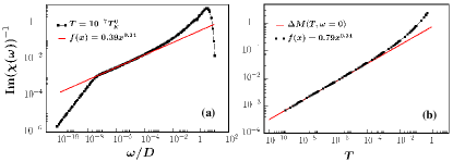
Figure 2: (a) $\mbox{Im}\big{(}\chi^{-1}_{\mbox{\tiny loc}}(\omega,T)\big{)}$ displays power law behavior $\sim\omega^{1-\epsilon}$ for $\omega>T$. (b) temperature dependent part of the saddle point self-energy $\Delta M(T,\omega=0)\sim T^{1-\epsilon}$.

The qualitative difference caused by the Berry phase term implies that the quantum interference effect is important for the universal properties of the QCP in the spin-isotropic BFKM. This is a natural manifestation of the fact that the Kondo effect – the formation of a Kondo singlet state and its critical destruction – involves the quantum entanglement of the local moment and spins of the conduction electrons. By bringing out the explicit effect of the Berry phase term, the spin-isotropic BFKM represents a prototype case in which the breakdown of the quantum-to-classical mapping can be studied. The situation in the Ising-anisotropic cases Vojta et al. (2005); Glossop and Ingersent (2005); Kirchner and Si ; Winter et al. is not as clear-cut. Still, since the SU(2) symmetry is restored in the Kondo screened phase of any spin-anisotropic Kondo system, it is plausible that related effects also come into play in the quantum criticality of the spin-anisotropic dissipative Kondo-like models.

In summary, we have analyzed the influence of the Berry phase, the topological phase term of the spin path integral, on the quantum critical properties of the Bose-Fermi Kondo model. We have done so using large-$N$ approaches based on appropriate generalizations of the model with and without the Berry phase term, and taking into account effects beyond the leading order in $1/N$. Without the Berry phase term, an interacting fixed point with the $\omega/T$-scaling occurs for $0<\epsilon<1/2$ but a Gaussian fixed point spoiling the $\omega/T$-scaling arises for $1/2\leq\epsilon<1$. With the Berry phase term, the Bose-Fermi Kondo model shows an interacting fixed point with $\omega/T$-scaling over the entire range $0<\epsilon<1$.

We thank C. J. Bolech, A. Inomata, S. Yamamoto and L. Zhu for useful discussions. This work has been supported in part by NSF Grant No. DMR-0706625, the Robert A. Welch Foundation, the W. M. Keck Foundation, and the Rice Computational Research Cluster funded by NSF and a partnership between Rice University, AMD and Cray.

References

- Sachdev (1999) S. Sachdev, Quantum Phase Transitions (Cambridge Univ. Press, Cambridge, 1999).
- Si et al. (2001) Q. Si, S. Rabello, K. Ingersent, and J. Smith, Nature 413, 804 (2001).
- Coleman et al. (2001) P. Coleman, C. Pépin, Q. Si, and R. Ramazashvili, J. Phys. Cond. Matt. 13, R723 (2001).
- v. Löhneysen et al. (2007) H. v. Löhneysen, A. Rosch, M. Vojta, and P. Wölfle, Rev. Mod. Phys. 79, 1015 (2007).
- Gegenwart et al. (2008) P. Gegenwart, Q. Si, and F. Steglich, Nat. Phys. 4, 186 (2008).
- Zhu and Si (2002) L. Zhu and Q. Si, Phys. Rev. B 66, 024426 (2002).
- Zaránd and Demler (2002) G. Zaránd and E. Demler, Phys. Rev. E 66, 024427 (2002).
- Zhu et al. (2004) L. Zhu, S. Kirchner, Q. Si, and A. Georges, Phys. Rev. Lett. 93, 267201 (2004).
- Vojta et al. (2005) M. Vojta, N.-H. Tong, and R. Bulla, Phys. Rev. Lett. 94, 070604 (2005).
- Glossop and Ingersent (2005) M. T. Glossop and K. Ingersent, Phys. Rev. Lett. 95, 067202 (2005).
- (11) S. Kirchner and Q. Si, arXiv:0808.0916.
- (12) A. Winter, H. Rieger, M. Vojta, and R. Bulla, arXiv:0807.4716.
- (13) M. Guidon, P. Werner, and M. Troyer, (unpublished).
- Perelomov (1986) A. Perelomov, Generalized Coherent States and Their Applications (Springer-Verlag, 1986).
- Inomata et al. (1992) A. Inomata, Path Integrals and coherent states of SU(2) and SU(1,1) (World Scientific, 1992).
- Parcollet and Georges (1998) O. Parcollet and A. Georges, Phys. Rev. B 58, 3794 (1998).
- Fisher et al. (1972) M. E. Fisher, S. Ma, and B. G. Nickel, Phys. Rev. Lett. 29, 917 (1972).
- Nemoto (2000) K. Nemoto, J. Phys. A 33, 3493 (2000).
- Mathur and Mani (2002) M. Mathur and H. S. Mani, J. Math. Phys. 43, 5351 (2002).
- Read and Sachdev (1989) N. Read and S. Sachdev, Nucl. Phys. B 316, 609 (1989).
- Cox and Ruckenstein (1993) D. L. Cox and A. L. Ruckenstein, Phys. Rev. Lett. 71, 1613 (1993).
- (22) for SU(2) coherent states can be any of the 2s+1 states with . Customary choices are or , so that the coherent states can be generated by either or alone. The determination of the normalizing factor which gives rise to the Berry phase in the path integral requires the proper use of the Baker-Cambell-Hausdorf formula in analogy to bosonic coherent states, .