Quantum-entanglement aspects of polaron systems

Abstract

We describe quantum entanglement inherent to the polaron ground states of coupled electron-phonon (or, more generally, particle-phonon) systems based on a model comprising both local (Holstein-type) and nonlocal (Peierls-type) coupling. We study this model using a variational method supplemented by the exact numerical diagonalization on a system of finite size. By way of subsequent numerical diagonalization of the reduced density matrix, we determine the particle-phonon entanglement as given by the von Neumann and linear entropies. Our results are strongly indicative of the intimate relationship between the particle localization/delocalization and the particle-phonon entanglement. In particular, we find a compelling evidence for the existence of a nonanalyticity in the entanglement entropies with respect to the Peierls-coupling strength. The occurrence of such nonanalyticity – not accompanied by an actual quantum phase transition – reinforces analogous conclusion drawn in several recent studies of entanglement in the realm of quantum-dissipative systems. In addition, we demonstrate that the entanglement entropies saturate inside the self-trapped region where the small-polaron states are nearly maximally mixed.

I Introduction

In recent years entangled quantum systems Ple ; Bengtsson and Życzkowski (2006) have garnered interest as a resource for quantum information processing. Bennett (1995) In addition, a great deal of research effort has been expended towards clarifying the role of entanglement in the (zero-temperature) quantum phase transitions of many-particle systems. Ost ; Galindo and Martin-Delgado (2002); Wu et al. (2006) Perhaps the most compelling, however, is the need to elucidate its possible bearing on the macroscopic properties of physical systems. ved ; Fac Namely, while the entanglement entropies are simply related to the many-body density matrix of the system, they bear no a priori relation to any observable physical quantity. Attempts to associate a physical meaning with entanglement were made, for example, in mesoscopic physics: schemes have been proposed for detection Choi et al. (2000) and even measurement of entanglement by exploiting its emergent relation to the quantum noise. mes ; Beenakker (2006)

Central to all the above developments is the problem of quantifying entanglement in diverse physical systems, such as quantum spin chains, Verstraete et al. (2004); Garcia-Ripoll et al. (2004); Fan et al. (2004) interacting bosons and/or fermions, Brandão (2005); Larsson and Johannesson (2005); Vollbrecht and Cirac (2007); Bañuls et al. (2007) quantum-dissipative sta ; Le Hur (2008) and disordered systems, Kopp et al. (2007) to name but a few. Ami In this regard, one of the areas of condensed-matter physics whose quantum-entanglement aspects have heretofore received only scanty consideration is that of the polaron problem. Ever since its inception by Landau and Pekar, lan the polaron concept Firsov (1975); Alexandrov and Mott (1995); Pol – a quantum particle interacting with a bosonic environment – has played an immensely important role in theoretical studies of coupled electron– or exciton–phonon (henceforth e-ph) systems. pol (a) What is more, this truly ubiquitous concept is lately finding resurgence in seemingly unrelated physical situations, the realm of ultracold atoms being a case in point. Col

The main body of polaron-related work is focussed on the study of a single electron interacting with the harmonic lattice vibrations through a short-range, non-polar potential that is linear in the lattice displacements and describes the dependence of the electronic on-site energies on the lattice degrees of freedom. The traditional starting point in describing such interaction, dubbed local e-ph coupling, is the paradigmatic molecular-crystal model due to Holstein. pol (a) As is being amply appreciated lately, pol (b); Perroni et al. (2004, 2005) however, local coupling is not the only type of short-range e-ph interaction relevant in realistic systems: nonlocal (off-diagonal) e-ph coupling accounts for the phonon-modulation of the electronic hopping integrals and bears relevance to several classes of molecule-based systems. The most common form of nonlocal coupling is Peierls-type coupling, Zaanen and Littlewood (1994); Zaanen (1996); Yonemitsu and Maeshima (2007) widely studied within the framework of the semi-classical Su-Schrieffer-Heeger (SSH) model SSH ; Zoli (2007); zol that describes the anomalous transport properties of nonlinear excitations (solitons, polarons) along the quasi-one-dimensional polyacetilene chain. In an implicit way – becoming manifest by carrying out the Jordan-Wigner transformation – this coupling forms the basis of the $XY$ spin-Peierls model, Cross and Fisher (1979); Barford and Bursill (2005) hence the name. Likewise, coupling to the breathing mode in cuprate superconductors is of Peierls’ type and – as transpires from recent investigations based on generalizations of the $t-J$ model – plays an important role in these systems, especially in the regime of weak doping. pol (b) Somewhat different forms of nonlocal coupling have been shown to be of relevance for charge transport in organic molecular crystals, Hannewald et al. (2004); Stojanović et al. (2004) carbon nanotubes, FoaTorres and Roche (2006) and DNA wires. Schmidt et al. (2007) It is worth of mention that a form of nonlocal coupling has also been incorporated in a generic electron-boson coupling model recently proposed by Alvermann et al.. Alvermann et al. (2007)

Given the abiding interest in the polaron problem in condensed-matter physics, the quantum-entanglement aspects of this problem have so far not been given due attention. While the changeover from a small to a large polaron is known to have the nature of a smooth crossover (with no broken symmetry), rather than a phase transition, Ger it is still tempting to quantify it using the entanglement measures. Entanglement in the one-dimensional Holstein model was studied by Zhao et al. Zhao et al. (2004) The authors emphasized the relation between the self-trapping process and the quantum (hetero-) entanglement between the phonon subsystem and electronic excitation. Effects of Peierls-type coupling, however, are as yet totally unexplored; given the wealth of intriguing implications of such interaction it appears interesting to elucidate the role it plays in particle localization as seen through entanglement measures. Additional motivation comes from recent investigations of entanglement in the realm of quantum dissipative systems. sta ; Le Hur (2008) One of the most important conclusions of these studies is that entanglement measures can have non-analyticities away from any phase transition and that these non-analyticities are intimately related to the loss of coherence. To be more specific, Stauber and Guinea sta found a nonanalyticity at the transition from underdamped to overdamped oscillations in the Ohmic case Porras et al. (2008) of the spin-boson model. Moreover, this nonanalyticity proved to be even more pronounced than the one occurring at the actual localization phase transition.

As a matter of fact, an evidence that non-analytic behavior of entanglement-related quantities does not necessarily coincide with the quantum phase transitions had already been found before. Ost Besides, a study of localizable entanglement in a gapped quantum spin system Verstraete et al. (2004) has showed that entanglement length diverges despite the fact that the correlation length remains finite, the latter indicating absence of a quantum phase transition. On the other hand, in disordered systems, for example, no such cases have been reported. It is therefore of interest to investigate whether the polaron problem – somewhat related to the spin-boson model, but with no phase transitions taking place – may also defy the tenet whereby an occurrence of a nonanalyticity in the entanglement entropy is a telltale signature of a quantum phase transition.

In the present work, we study entanglement in polaron systems. In order to address the problem from as general a viewpoint as possible, we start from a polaron model that includes both local (Holstein-type) and nonlocal (Peierls-type) short-range e-ph coupling. Given that this Hamiltonian does not admit an exact solution in any physically-relevant limit, we analyze it using a variational method supplemented by an exact diagonalization on a finite-size system. Proceeding in this way, we find that entanglement exhibits non-analyticities as a function of Peierls-type coupling, which are not accompanied by a phase transition. We argue that the occurrence of such “accidental” nonanalyticities in the problem at hand is related to the loss of coherence, much like in the quantum-dissipative systems.

The outline of the remainder of this paper is as follows. In Sec. II we present the model and notation to be used throughout. Sec. III contains details of our variational approach: we first introduce our variational Ansatz, then provide details of analytical derivations needed to implement it, and finally describe our computational method of variational minimization. The following Sec. IV contains essential details of the exact diagonalization method. In Sec. V we introduce the entanglement measures and lay out the method for calculating them. The obtained results are presented in Sec. VI, accompanied by a discussion of their salient features. We conclude, with some general remarks, in Sec. VII.

II Model

The system under study consists of an excess particle (electron, hole, exciton) interacting with harmonic lattice vibrations – dispersionless (Einstein) phonons – through a short-range interaction. As our starting point, we adopt a one-dimensional e-ph Hamiltonian obtained by dovetailing the Peierls-type coupling term on the conventional Holstein Hamiltonian. (Restriction to a one-dimensional system is not a severe limitation given the short-range nature of the e-ph interactions discussed here.) The compact form of this extended Holstein model reads

$$\hat{H}=\sum_{i}\varepsilon_{i}(\{\hat{\mathbf{u}}\})\>\hat{a}_{i}^{\dagger}\hat{a}_{i}+\sum_{i}t_{i+1,i}(\{\hat{\mathbf{u}}\})\>(\hat{a}_{i+1}^{\dagger}\hat{a}_{i}+\mathrm{h.c.})\\ +\omega\sum_{i}\>\hat{b}_{i}^{\dagger}\hat{b}_{i}\>,$$ (1)

where $\hat{a}_{i}^{\dagger}$($\hat{a}_{i}$) creates (destroys) a particle at $i$-th site (at position $R_{i}$, $i=0,1,\ldots,N-1$), $\hat{b}_{i}^{\dagger}$($\hat{b}_{i}$) creates (destroys) a dispersionless phonon with frequency $\omega$ at the same site. The effective on-site energy

$$\varepsilon_{i}(\{\hat{\mathbf{u}}\})=\varepsilon+{\alpha}_{\scriptscriptstyle H}\hat{u}_{i}\>,$$ (2)

and hopping integral

$$t_{i+1,i}(\{\hat{\mathbf{u}}\})=-t+{\alpha}_{\scriptscriptstyle P}(\hat{u}_{i+1}-\hat{u}_{i})\>,$$ (3)

depend on the lattice displacements $\hat{u}_{i}\equiv(2M\omega)^{-\scriptscriptstyle 1/2}(\hat{b}_{i}+\hat{b}_{i}^{\dagger})$, where ${\alpha}_{\scriptscriptstyle H}$ and ${\alpha}_{\scriptscriptstyle P}$ are the local (Holstein-type) and nonlocal (Peierls-type) coupling constants, respectively, and $M$ is the mass of molecules in the underlying crystal. The bare on-site energy and hopping integral are denoted by $\varepsilon$ and $t$, respectively. For simplicity we take $\varepsilon=0$ in what follows. More explicitly, the Hamiltonian can be written as

$$\hat{H}=\hat{H}_{\rm e}+\hat{H}_{\rm ph}+\hat{H}_{g}+\hat{H}_{\phi}\>,$$ (4)

where

$$\hat{H}_{\rm e} =-t\sum_{i}(\hat{a}^{\dagger}_{i+1}\hat{a}_{i}+\mathrm{h.c.})\>,$$ (5)

$$\hat{H}_{\rm ph} =\omega\sum_{i}\hat{b}^{\dagger}_{i}\hat{b}_{i}\>,$$ (6)

$$\hat{H}_{g} =g\omega\sum_{i}\hat{a}^{\dagger}_{i}\hat{a}_{i}(\hat{b}^{\dagger}_{i}+\hat{b}_{i})\>,$$ (7)

$$\hat{H}_{\phi} =\phi\omega\sum_{i}(\hat{a}^{\dagger}_{i+1}\hat{a}_{i}+\mathrm{h.c.})(\hat{b}^{\dagger}_{i+1}+\hat{b}_{i+1}-\hat{b}^{\dagger}_{i}-\hat{b}_{i})\>,$$ (8)

with $g\equiv{\alpha}_{\scriptscriptstyle H}/\sqrt{2M\omega^{3}}$ and $\phi\equiv{\alpha}_{\scriptscriptstyle P}/\sqrt{2M\omega^{3}}$ being the dimensionless local and nonlocal coupling constants, respectively. The two important limiting cases of our model are the Holstein model ($\phi=0$) and the quantized version of the SSH model ($g=0$).

The eigenstates of Hamiltonian (4) ought to be the good-quasi-momentum states, i.e., eigenstates of the total crystal momentum operator

$$\hat{K}=\sum_{k}k\>\hat{a}^{\dagger}_{k}\hat{a}_{k}+\sum_{q}q\>\hat{b}^{\dagger}_{q}\hat{b}_{q}\>\>,$$ (9)

since the latter commutes with $\hat{H}$. In the following, the eigenvalues of $\hat{K}$ will be labelled with $\kappa$. By making use of the Born-von Karman periodic boundary conditions, the quasi-momenta in the first Brillouin zone are given by $\kappa=(2\pi/a)(m/N)$ ($a$ – the lattice spacing; $m=0,1,\ldots,N-1$). For convenience, we express quasi-momenta in units of $a^{-1}$, so that $\kappa R_{n}=\kappa na\to\kappa n$.

III Variational method

III.1 Choice of variational Ansatz

While not being exactly-soluble, Hamiltonian in Eq. (4) can be treated variationally; in the studies of coupled e-ph systems methods of this type have been shown to yield quantitatively trustworthy results that compare well with those obtained by the exact (numerical) diagonalizations. Weiße et al. (2000); Ku et al. (2002) An important class of such methods is furnished by Toyozawa’s Ansatz state Toyozawa (1961) and generalizations thereof. Rom ; Ku et al. (2002); Barišić (2002) While these Ansatz states have been widely used in the studies of the Holstein model, they are also capable of describing systems with simultaneous local and nonlocal coupling.

Omitting the most conventional form of Toyozawa’s Ansatz state, we purposefully cast it in a way that renders manifest its entangled nature:

$$|\psi_{\kappa}\rangle=\frac{1}{N}\sum_{n,m}e^{i\kappa n}\gamma^{\kappa}_{m-n}\>\hat{a}_{m}^{\dagger}|0\rangle_{\textrm{e}}\otimes\prod_{l}\hat{D}_{l}(\xi_{l-n}^{\kappa})|0\rangle_{\textrm{ph}}\>,$$ (10)

where $|0\rangle_{\textrm{e}}$ ($|0\rangle_{\textrm{ph}}$) is the electron (phonon) vacuum, and $\hat{D}_{l}(\alpha)\equiv\exp(\alpha\hat{b}_{l}^{\dagger}-\alpha^{*}\hat{b}_{l})$ is Glauber’s displacement operator that creates the phonon coherent state $|\xi_{l-n}^{\kappa}\rangle_{\textrm{ph}}\equiv\hat{D}_{l}(\xi_{l-n}^{\kappa})|0\rangle_{\textrm{ph}}$ at site $l$. This (overcomplete) set of phonon coherent states captures the multi-phononic nature of the polaron ground state. Importantly, it is the dependence of the variational parameters $\gamma_{m-n}^{\kappa}$ on both $m$ and $n$ that renders Ansatz state $|\psi_{\kappa}\rangle$ entangled: the sums over these indices cannot be decoupled, implying that this state cannot be expressed as a separable (direct-product) state in the Hilbert space ${\mathcal{H}}={\mathcal{H}}_{\textrm{e}}\otimes{\mathcal{H}}_{\textrm{ph}}$.

Generally speaking, the use of variational methods invariably involves the trade-off between flexibility of the variational wave-function (which increases with the growing number of parameters) and numerical difficulty of finding reliably the global minimum of the ground-state-energy expectation value (complexity grows rapidly with parameter number; see Sec. III.2 for additional details). In this regard, the major drawback of Toyozawa’s Ansatz is that it involves a large number – $2N$ for each $\kappa$ – of variational parameters. Alternative methods have been proposed that provide accurate results, while involving smaller number of parameters. Adopting this point of view, we seek the polaron eigenstates of Hamiltonian (4) in the form of translationally-invariant Bloch states

$${|{\psi}_{\kappa}\rangle}=\frac{1}{\sqrt{N}}\sum_{n}e^{i\kappa n}\>{|{\psi}_{\kappa}(n)\rangle}\>,$$ (11)

with “form-factors” ${|{\psi}_{\kappa}(n)\rangle}$ given by Perroni et al. (2004)

$${|{\psi}_{\kappa}(n)\rangle}=\sum_{m}{\Phi}_{\kappa}(m)\;e^{i\kappa m}\>\hat{a}^{\dagger}_{n+m}{|0\rangle}_{\rm e}\\ \otimes\exp\Big{(}\sum_{j=-2}^{2}\hat{U}_{\kappa;j}(n+j)\Big{)}{|0\rangle}_{\rm ph}\>.$$ (12)

The skew-Hermitian operators $\hat{U}_{\kappa;j}$ ($j=0,\pm 1,\pm 2$) are defined as

$$\hat{U}_{\kappa;j}(n)=\frac{1}{\sqrt{N}}\sum_{q}\Big{(}f_{\kappa;j}(q)\;e^{iqn}\;\hat{b}_{q}-\textrm{h.c.}\Big{)}\>,$$ (13)

with

$$f_{\kappa;j}(q)=\frac{{\alpha}_{\kappa;j}}{1+2\;(t/\omega)\;{\beta}_{\kappa;j}[\cos(\kappa)-\cos(\kappa+q)]}\>.$$ (14)

Using trial wave-functions (11), the lowest polaron band $E_{\textrm{\tiny{GS}}}(\kappa)$ can be obtained by minimizing the energy expectation value over variational parameters $V_{\kappa}=\big{\{}{\alpha}_{\kappa;\scriptscriptstyle 0},{\alpha}_{\kappa;\scriptscriptstyle\pm 1},{\alpha}_{\kappa;\scriptscriptstyle\pm 2};{\beta}_{\kappa;\scriptscriptstyle 0},{\beta}_{\kappa;\scriptscriptstyle\pm 1},{\beta}_{\kappa;\scriptscriptstyle\pm 2};{\Phi}_{\kappa}(-5),\ldots,{\Phi}_{\kappa}(5)\big{\}}$:

$$E_{\textrm{\tiny{GS}}}(\kappa)=\min_{\displaystyle V_{\kappa}}\>\frac{\langle\psi_{\kappa}|\>\hat{H}\>|\psi_{\kappa}\rangle}{\langle\psi_{\kappa}|\psi_{\kappa}\rangle}\>.$$ (15)

[Note that for each $\kappa$ there are in total twenty variational parameters; this number is fixed, rather than being proportional to the system size as in Toyozawa’s Ansatz. Importantly, among eleven parameters ${\Phi}_{\kappa}(j)$ only ten are independent because of the normalization condition on the trial wave-function in Eq. (11).] In the following, we will be particularly interested in the polaron ground-state energy $E_{\textrm{\tiny{GS}}}(\kappa=0)\equiv E_{0}$. The corresponding variationally-optimized ground-state wave-function will hereafter be denoted with $|\textrm{GS}\rangle$.

III.2 Matrix elements and computational scheme

Here we present the derivation of the expression for the energy expectation value, followed by the details of our numerical method for variational minimization. To facilitate further derivations we first note that

$$\exp\Big{(}\sum_{j=-2}^{2}\hat{U}_{\kappa;j}(n+j)\Big{)}=\prod_{q}\hat{D}_{q}\Big{(}-\frac{e^{-iqn}w_{\kappa}^{*}(q)}{\sqrt{N}}\Big{)}\>,$$ (16)

where $\hat{D}_{q}(\alpha_{q})\equiv\exp(\alpha_{q}\hat{b}_{q}^{\dagger}-\alpha_{q}^{*}\hat{b}_{q})$ is Glauber’s displacement operator that creates a coherent state of phonons with quasi-momentum $q$, and $w_{\kappa}(q)$ is defined as

$$w_{\kappa}(q)\equiv\sum_{j=-2}^{2}f_{\kappa;j}(q)\>e^{iqj}\>.$$ (17)

It is straightforward to show that

$$\langle{\psi}_{\kappa}|{\psi}_{\kappa}\rangle=\sum_{mm^{\prime}}{\Phi}_{\kappa}^{*}(m^{\prime}){\Phi}_{\kappa}(m)\;Z^{\kappa}_{m-m^{\prime}}\>,$$ (18)

where

$$\begin{array}[]{rl}&\displaystyle Z^{\kappa}_{m-m^{\prime}}\equiv\\ &{}_{\textrm{\tiny{ph}}}\Big{\langle}0\Big{|}\prod_{q}\hat{D}_{q}^{\dagger}\Big{(}-\frac{e^{-iqm}w_{\kappa}^{*}(q)}{\sqrt{N}}\Big{)}\hat{D}_{q}\Big{(}-\frac{e^{-iqm^{\prime}}w_{\kappa}^{*}(q)}{\sqrt{N}}\Big{)}\Big{|}0\Big{\rangle}_{\textrm{\tiny{ph}}}\>.\end{array}$$ (19)

By making use of the well-known expression Scully and Zubairy (1997) for the overlap of coherent states $\langle\alpha|\beta\rangle$ ($\alpha,\beta\in\mathbb{C}$)

$${\langle\alpha|}\beta\rangle=\langle 0|\>\hat{D}^{\dagger}(\alpha)\hat{D}(\beta)\>|0\rangle=e^{\alpha^{*}\beta}\>e^{-\frac{1}{2}(|\alpha|^{2}+|\beta|^{2})}$$ (20)

we obtain

$$Z^{\kappa}_{m-m^{\prime}}=\exp\Big{[}-\frac{1}{N}\sum_{q}\Big{(}1-e^{iq(m-m^{\prime})}\Big{)}|w_{\kappa}(q)|^{2}\Big{]}\>.$$ (21)

Other relevant matrix elements are given by

$${\langle{\psi}_{\kappa}|}\;\hat{H}_{\rm e}\;{|{\psi}_{\kappa}\rangle}=-t\sum_{mm^{\prime}}{\Phi}_{\kappa}^{*}(m^{\prime}){\Phi}_{\kappa}(m)\\ \times\Big{(}e^{-i\kappa}\>Z^{\kappa}_{m-m^{\prime}+1}+e^{i\kappa}\>Z^{\kappa}_{m-m^{\prime}-1}\Big{)}\>,$$ (22)

$${\langle{\psi}_{\kappa}|}\;\hat{H}_{\rm ph}\;{|{\psi}_{\kappa}\rangle}=\frac{\omega}{N}\sum_{mm^{\prime}}{\Phi}_{\kappa}^{*}(m^{\prime}){\Phi}_{\kappa}(m)\;Z^{\kappa}_{m-m^{\prime}}\\ \times\sum_{q}e^{iq(m-m^{\prime})}\;|w_{\kappa}(q)|^{2}\>,$$ (23)

$${\langle{\psi}_{\kappa}|}\;\hat{H}_{g}\;{|{\psi}_{\kappa}\rangle}=-\frac{g\omega}{N}\sum_{mm^{\prime}}{\Phi}_{\kappa}^{*}(m^{\prime}){\Phi}_{\kappa}(m)\;Z^{\kappa}_{m-m^{\prime}}\\ \times\sum_{q}\Big{(}e^{-iqm^{\prime}}w_{\kappa}(q)+e^{iqm}w_{\kappa}^{*}(q)\Big{)}\>,$$ (24)

$${\langle{\psi}_{\kappa}|}\;\hat{H}_{\phi}\;{|{\psi}_{\kappa}\rangle}=\frac{\phi\omega}{N}\sum_{mm^{\prime}}{\Phi}_{\kappa}^{*}(m^{\prime}){\Phi}_{\kappa}(m)\sum_{q}\\ \times\Big{(}e^{i\kappa}\;Z^{\kappa}_{m-m^{\prime}-1}(1-e^{-iq})-e^{-i\kappa}\;Z^{\kappa}_{m-m^{\prime}+1}(1-e^{iq})\Big{)}\\ \times\Big{(}e^{-iqm^{\prime}}w_{\kappa}(q)-e^{iqm}w_{\kappa}^{*}(q)\Big{)}\>.$$ (25)

The above formulae are easily derived using identity

$$e^{\hat{A}}e^{\hat{B}}=e^{\hat{A}+\hat{B}}e^{\frac{1}{2}[\hat{A},\hat{B}]}\>,$$ (26)

which holds if operators $\hat{A}$ and $\hat{B}$ satisfy condition $[\hat{A},[\hat{A},\hat{B}]]=[\hat{B},[\hat{A},\hat{B}]]=0$, as well as identity

$$\big{[}\>\hat{b},f(\hat{b}^{\dagger},\hat{b})\>\big{]}=\frac{\partial f(\hat{b}^{\dagger},\hat{b})}{\partial\hat{b}^{\dagger}}\>,$$ (27)

valid for an arbitrary analytic function $f(\hat{b}^{\dagger},\hat{b})$ of bosonic operators.

An important measure of the multi-phononic nature of the polaron ground state is the average number of phonons

$$\bar{N}_{\textrm{ph}}=\>\Big{\langle}\textrm{GS}\Big{|}\>\sum_{i}\hat{b}_{i}^{\dagger}\hat{b}_{i}\Big{|}\textrm{GS}\Big{\rangle}\>,$$ (28)

which can be obtained using Eq. (23).

Based on the expressions for $\langle\psi_{\kappa}|\>\hat{H}\>|\psi_{\kappa}\rangle$ and $\langle\psi_{\kappa}|\psi_{\kappa}\rangle$, we perform variational minimization in order to find the polaron ground state ($\kappa=0$) for a system with $N=32$ sites. Due to the large number ($n=20$) of variational parameters involved, the energy expectation value is a function of these parameters with multiple local minima. Finding the global minimum thus constitutes a rather nontrivial numerical optimization problem. We perform this complex task using the multi-start-based global random search method: Törn and Žilinskas (1989) we first generate a large sample ($\sim 10^{5}$) of random points in the space of variational parameters; we then select a smaller number ($\sim 20$) of them that have the smallest values of the function to be minimized and perform local searches for minima [$O(n^{3})$ computation] around each of these points: the one with the smallest energy is then adopted as the sought-after global minimum. The fidelity of this approach is corroborated by the stability of the final result for the global minimum upon varying the initial number of random points.

Regarding the choice of our numerical method a remark is in order here. In the local-coupling-only case ($\phi=0$, i.e., the Holstein model), the system is exactly soluble in the “unphysical” limit of zero hopping ($t\rightarrow 0$) by the well-known Lang-Firsov canonical transformation. pol (a) The natural way to proceed in finding the optimal variational parameters for finite $t$ is then to start from the exact solution for $t=0$ and gradually change $t$, using optimal values of variational parameters obtained for given value of $t$ as the initial guess for the next, slightly higher value. However, for finite $\phi$ the model is not exactly-soluble in any relevant limit. Therefore, the procedure just described does not carry over to the $\phi\neq 0$ case and one needs a careful sampling of the entire space of variational parameters, afforded by the multi-start-type methods, to reliably find the global minimum of the ground-state-energy expectation value.

III.3 Application scope of our variational method and comparison with other methods

While Ansatz state in Eqs. (11)-(12) was originally introduced for use in the Peierls-coupling-only case (quantized SSH model), we here demonstrate the that it can also be utilized for the local-coupling-only case (Holstein model), and accordingly for the case with simultaneous local and nonlocal couplings. The nearly-perfect agreement of our results in the $\phi=0$ case with another known variational approach, suggested by Cataudella et al. Cataudella et al. (1999), is illustrated in Fig. 1a,b. The latter was shown to agree well with the Global-Local method Rom implying the general agreement of all three methods. Therefore the trial states used here are generally applicable to short-ranged e-ph interactions with Einstein phonons. The agreement between the results obtained by the variational methods of the present type and other approaches (density-matrix renormalization group method, Jeckelmann and White (1998) quantum Monte Carlo Pol ) is also well established. Rom

FIG. 1: Comparison of the ground-state energies obtained using the variational method of Cataudella et al. Cataudella et al. (1999) (circles) and the method of the present work (solid curve) in the $\phi=0$ case: $t/\omega=1.0$ (a) and $t/\omega=2.0$ (b).

IV Exact diagonalization

To supplement our variational method, we also perform an exact numerical diagonalization of Hamiltonian (4) on a system of finite size. We study system of $N=6$ sites, varying the maximal number of phonons between $M=8$ and $M=10$. The states in the truncated Hilbert space are given by

$$|\Psi\rangle=\sum_{\mathbf{n},\mathbf{m}}C_{\mathbf{n,m}}\>|\mathbf{n}\rangle\otimes|\mathbf{m}\rangle\>,$$ (29)

where $\mathbf{n}=(n_{\scriptscriptstyle 0},...,n_{\scriptscriptstyle N-1})$ and $\mathbf{m}=(m_{\scriptscriptstyle 0},...,m_{\scriptscriptstyle N-1})$ are the sitewise electron and phonon occupation numbers ($\sum_{i}n_{i}=1,\>\sum_{i}m_{i}\leq M$). Coefficients $C_{\mathbf{n,m}}$ contain the information about the phonon content of state $|\Psi\rangle$.

FIG. 2: Phonon distribution sitewise in the polaron ground state for $t/\omega=1.0$, $\phi=1.3$ ($N=6$, $M=10$). The states $\mathbf{m}$ with the same total number of phonons $m=\sum_{i}m_{i}$ are indicated by the bins at the bottom portion of the plot.

One of the crucial prerequisites for a successful application of the exact-diagonalization approach in the present context is a proper truncation of the (otherwise infinite-dimensional) phonon Hilbert space. In other words, the maximal total number of phonons on a lattice has to be large enough as to be capable to account for the phonon distribution in the polaron ground state in the strong-coupling regime. Typical phonon content (sitewise) of the polaron ground state obtained by exact diagonalization is illustrated in Fig. 2, where the $n$-th group of peaks represents the phonon distribution for the case when the electron is located at site $n$ ($n=0,...,N-1$). Within each group of peaks, coefficients $C_{\mathbf{n},\mathbf{m}}$ are given in the ascending order of the phonon occupation numbers. For weak coupling, phonon distribution $p_{m}=\sum_{\mathbf{m}}|C_{\mathbf{n},\mathbf{m}}|^{2}$ (where $m=\sum_{i}m_{i}$) peaks at $m=0$ phonons, while in the strong-coupling regime it peaks at $m=3$ or $4$ phonons. This a posteriori corroborates that our choice of the maximal number of phonons (between $8$ and $10$) was pertinent.

V Entanglement

V.1 Entanglement entropies: generalities

In order to make the present work self-contained, before embarking on the calculation of entanglement in our coupled e-ph system we review the general prescription for characterization of bipartite quantum entanglement. We consider a composite quantum system that can be divided up into two parts A and B, where A denotes the subsystem of interest and B the environment whose details are unimportant. The Hilbert space of the full system has the form of a tensor product: $\mathcal{H}=\mathcal{H}_{\textrm{\tiny{A}}}\otimes\mathcal{H}_{\textrm{\tiny{B}}}$. In a pure state $|\Psi\rangle$, the density matrix of the full system is given by

$$\hat{\rho}=\frac{|\Psi\rangle\langle\Psi|}{\langle\Psi|\Psi\rangle}\>.$$ (30)

We then construct the reduced (marginal) density matrix $\hat{\rho}_{\textrm{\tiny{A}}}$ by tracing over the environmental degrees of freedom: $\hat{\rho}_{\textrm{\tiny{A}}}=\mathop{Tr}_{\textrm{\tiny{B}}}\hat{\rho}$. The von Neumann (entanglement) entropy, defined by

$$S=-\textrm{Tr}_{\textrm{\tiny{A}}}(\hat{\rho}_{\textrm{\tiny{A}}}\ln\hat{\rho}_{\textrm{\tiny{A}}})\>,$$ (31)

contains information about the quantum correlations present in the pure quantum state under study. It represents the most widely used measure of bipartite quantum entanglement. Note that $S=-\mathop{Tr}_{\textrm{\tiny{A}}}(\hat{\rho}_{\textrm{\tiny{A}}}\ln\hat{\rho}_{\textrm{\tiny{A}}})=-\mathop{Tr}_{\textrm{\tiny{B}}}(\hat{\rho}_{\textrm{\tiny{B}}}\ln\hat{\rho}_{\textrm{\tiny{B}}})$, where the reduced density matrix $\hat{\rho}_{\textrm{\tiny{B}}}$ is obtained by tracing over the degrees of freedom in subsystem A. The upper bound $S_{\textrm{max}}=\ln(D)$ of $S$, where $D$ is dimensionality of the reduced density matrix, is reached when the reduced density matrix is maximally mixed.

The so-called linear entropy is defined as

$$S_{\scriptscriptstyle L}=1-\textrm{Tr}_{\textrm{\tiny{A}}}(\hat{\rho}^{2}_{\textrm{\tiny{A}}})\>,$$ (32)

and has the advantage (compared to the von Neumann entropy) of being easier to calculate. It is worth of mention that both the von Neumann and linear entropies are closely related to the quantum Rényi entropies Bengtsson and Życzkowski (2006) $S_{q}(\hat{\rho})\equiv(1-q)^{-1}\ln(\textrm{Tr}\hat{\rho}^{q})$ ($q\geq 0$): $S(\hat{\rho})$ is the $q\rightarrow 1$ limit of $S_{q}(\hat{\rho})$, while $S_{\scriptscriptstyle L}(\hat{\rho})$ is simply related to $S_{2}(\hat{\rho})$. The upper bound of $S_{\scriptscriptstyle L}$, reached for the maximally-mixed reduced density matrix, is given by $S_{{\scriptscriptstyle L},\textrm{max}}=1-D^{-1}$.

V.2 Reduced density matrix from variational approach

In accordance with general relation (30), the density matrix corresponding to the state $|\psi_{\kappa}\rangle$ on the tensor-product Hilbert space ${\mathcal{H}}={\mathcal{H}}_{\textrm{e}}\otimes{\mathcal{H}}_{\textrm{ph}}$ is given by

$$\hat{\rho}_{\textrm{e-ph}}(\kappa)=\frac{|\psi_{\kappa}\rangle\langle\psi_{\kappa}|}{\langle\psi_{\kappa}|\psi_{\kappa}\rangle}\>.$$ (33)

The reduced particle (electron) density matrix is given by the partial trace over the phonon Hilbert space ${\mathcal{H}}_{\textrm{ph}}$:

$$\hat{\rho}_{\textrm{e}}(\kappa)=\textrm{Tr}_{\textrm{ph}}\big{[}\hat{\rho}_{\textrm{e-ph}}(\kappa)\big{]}\>.$$ (34)

Straightforward derivation, with the aid of Eq. (19), yields

$$\begin{array}[]{rl}&\displaystyle\textrm{Tr}_{\textrm{ph}}\big{(}{|{\psi}_{\kappa}\rangle}{\langle{\psi}_{\kappa}|}\big{)}=\frac{1}{N}\sum_{nn^{\prime}}\>\Big{(}\sum_{m,m^{\prime}}\Phi_{\kappa}^{*}(m^{\prime})\Phi_{\kappa}(m)\\ &\displaystyle\times\>Z^{\kappa}_{m-m^{\prime}+n^{\prime}-n}\Big{)}\>e^{i\kappa(n-n^{\prime})}{|n\rangle}_{\textrm{e}}\>{}_{\textrm{e}}{\langle n^{\prime}|}\>,\end{array}$$ (35)

where ${|n\rangle}_{\textrm{e}}\equiv a^{\dagger}_{n}|0\rangle_{\textrm{e}}$ is the state with electron at site $n$. The last equation, when combined with Eq. (18), readily leads to the expression for the general matrix element of the reduced density matrix $\hat{\rho}_{\textrm{e}}(\kappa=0)\equiv\hat{\rho}_{\textrm{e}}$ in the polaron ground state:

$$\big{(}\hat{\rho}_{\textrm{e}}\big{)}_{nn^{\prime}}=\frac{1}{N}\frac{\sum_{\scriptscriptstyle mm^{\prime}}\Phi_{\kappa\scriptscriptstyle=0}^{*}(m^{\prime})\Phi_{\kappa\scriptscriptstyle=0}(m)\;Z^{\kappa\scriptscriptstyle=0}_{m-m^{\prime}+n^{\prime}-n}}{\sum_{\scriptscriptstyle mm^{\prime}}{\Phi}_{\kappa\scriptscriptstyle=0}^{*}(m^{\prime}){\Phi}_{\kappa\scriptscriptstyle=0}(m)\;Z^{\kappa\scriptscriptstyle=0}_{m-m^{\prime}}}\>.$$ (36)

The corresponding von Neumann entropy

$$S=-\textrm{Tr}_{\textrm{e}}(\hat{\rho}_{\textrm{e}}\ln\hat{\rho}_{\textrm{e}})$$ (37)

can be expressed as

$$S=-\sum_{i}\lambda_{i}\ln\lambda_{i}\>,$$ (38)

where $\left\{\lambda_{i}\>|\>i=0,1,\ldots,N-1\right\}$ are the eigenvalues ($\lambda_{i}>0\>,\>\sum_{i}\lambda_{i}=1$) of $\hat{\rho}_{\textrm{e}}$. Based on our variational approach, the linear entropy

$$S_{\scriptscriptstyle L}=1-\textrm{Tr}_{\textrm{e}}(\hat{\rho}_{\textrm{e}}^{2})$$ (39)

can readily be obtained in an analytical form using Eq. (36); however, we here omit the ensuing cumbersome expression. In the exact-diagonalization approach, the reduced density matrix $\hat{\rho}_{\textrm{e}}$ is obtained from the corresponding eigenvectors. The results illustrating dependence of the entanglement entropies on the e-ph coupling strengths are presented in the following section.

VI Results and Discussion

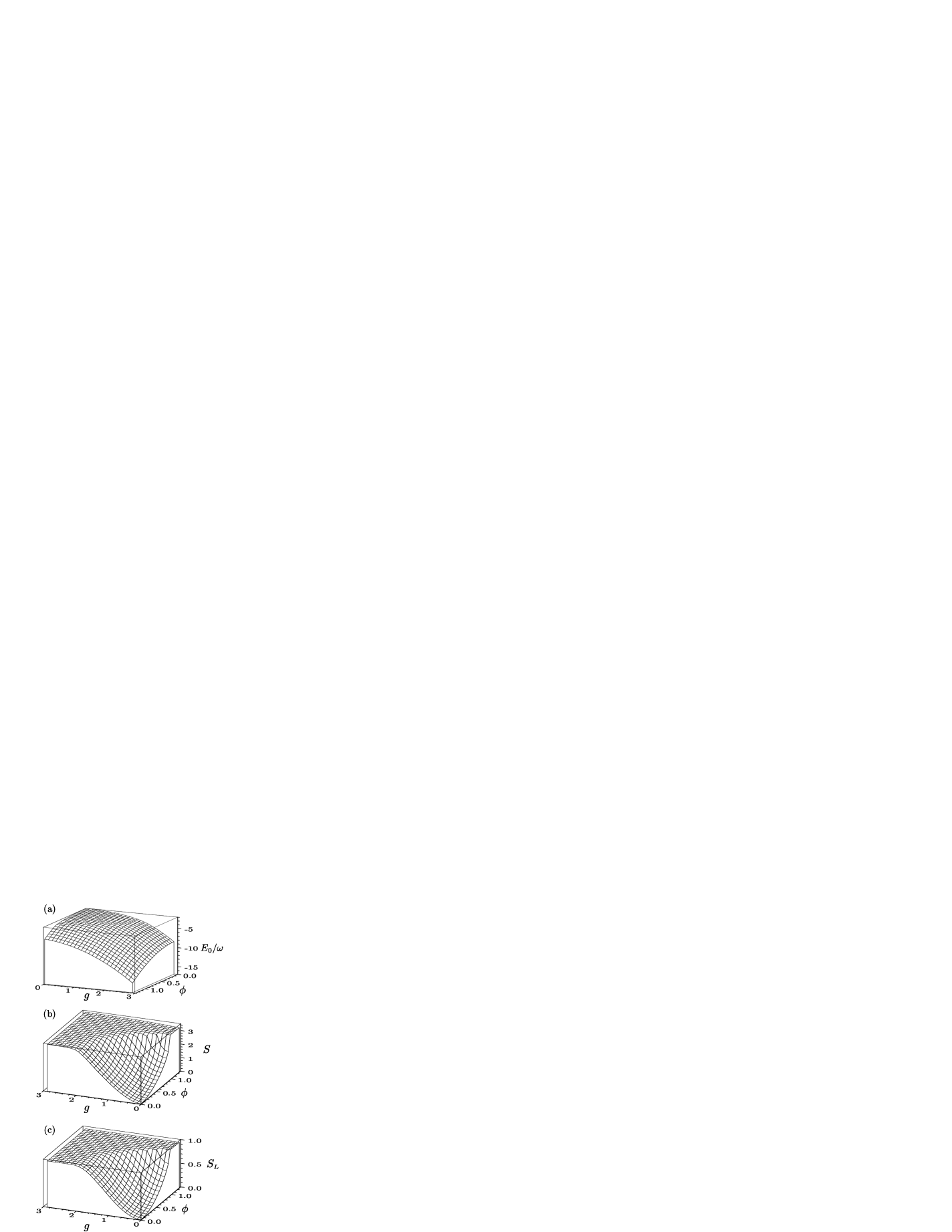
FIG. 3: Variational ground-state energy (a), the von Neumann entropy (b), and linear entropy (c) as functions of dimensionless local ($g$) and nonlocal ($\phi$) coupling strengths, for $t/\omega=1.0$ and $N=32$.

Our numerical results, obtained using variational approach, correctly reproduce a continuous dependence of the polaron ground-state energy, displayed in Fig. 3a for $t/\omega=1.0$, on local and nonlocal coupling strengths, reflecting the well-known absence of phase transitions in coupled e-ph systems. Ger

The entanglement entropies, depicted in Fig. 3b,c for $t/\omega=1.0$, both behave in a similar way: they increase with increasing coupling strengths, saturating and remaining essentially unchanged in the self-trapped region where the particle becomes localized. The saturation values of the two entropies are close to those of the maximally-mixed density matrix: $S_{\textrm{max}}=\ln(N)$, $S_{{\scriptscriptstyle L},\textrm{max}}=1-N^{-1}$. For example, for $N=32$, $S_{\textrm{max}}=3.46$, $S_{{\scriptscriptstyle L},\textrm{max}}=0.97$ (cf. Fig. 3).

Importantly, for $t/\omega\gtrsim 0.85$ we find a strong nonanalyticity in the dependence of entanglement entropies on the nonlocal coupling strength. This nonanalyticity has the character of a jump-discontinuity and is more pronounced in the case of von Neumann entropy (Fig. 3b) than for the linear entropy (Fig. 3c). It becomes more and more pronounced with increasing value of $t/\omega$, i.e., upon approaching the adiabatic regime $t\gg\omega$. In order to emphasize that discontinuous behavior sets in for sufficiently large value of the ratio $t/\omega$, in Fig. 4a we depict the von Neumann entropy for $t/\omega=0.25$ where the nonanalyticity does not exist at all, and for $t/\omega=2.0$ (Fig. 4b) where the nonanalyticity is noticeably more pronounced than for $t/\omega=1.0$.

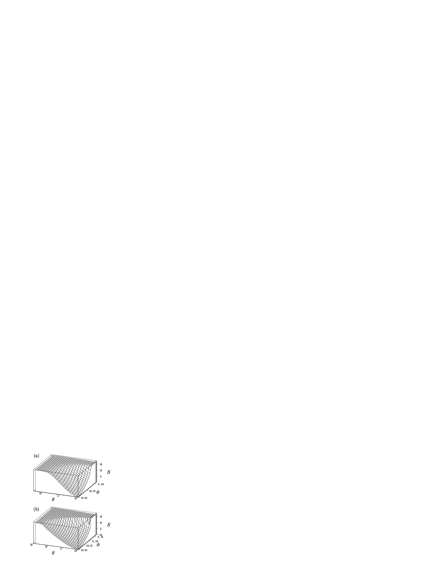
FIG. 4: The von Neumann entropy $S$, obtained variationally, as a function of dimensionless local ($g$) and nonlocal ($\phi$) coupling strengths. Displayed are results for $t/\omega=0.25$ (a) and $t/\omega=2.0$ (b), with $N=32$.

To emphasize the appearance of a nonanalyticity in the entanglement entropies as a function of nonlocal coupling strength, we study the nonlocal-coupling-only case making comparisons between the results of the two approaches (variational and exact diagonalization). Typical results are depicted in Fig. 5. Figure 5a illustrates very good agreement between the two approaches as far as the ground-state energy is concerned. In Figs. 5b,c the entanglement entropies are shown as obtained from two different variational calculations (for $N=6$ and $N=32$) and two different exact-diagonalizations (with $N=6$ and maximum $M=8$ or $10$ phonons used). The only sizeable discrepancy is in the behavior of $S$, which clearly stems from the finite-size effects: while values of $S$ corresponding to the variational calculation with $N=32$ deviate considerably from those of exact diagonalizations with $N=6$, the difference between the two approaches when applied to a system with the same number of sites is not very drastic. However, the most important feature of the obtained results, manifest in all the cases considered, is the non-analytic behavior of $S$ and $S_{\scriptscriptstyle L}$ with respect to $\phi$.

Detailed analysis shows that the observed nonanalyticities occur for values of $\phi$ at which the lowest energy states of $\hat{H}(\phi)$ undergo avoided crossings. The crossings are avoided (rather than real ones) because $[\hat{H},\hat{H}_{\phi}]\neq 0$, Sachdev (1999) leading to a smooth dependence of the polaron ground-state energy on the coupling strength $\phi$ (and, accordingly, the absence of a phase transition in the conventional sense of the term). There is, however, no general principle that would rule out the occurrence of nonanalyticities in the entanglement entropies at these avoided-crossing points.

FIG. 5: Ground-state energy (a), the von Neumann entropy (b), and linear entropy (c) for $t/\omega=1.0$ and $g=0$, as calculated using the variational (var.) and exact diagonalization (e.d.) approaches. $N$ is the number of sites, while $M$ stands for the maximal number of phonons used for exact diagonalization. The arrows indicate the entropies for the maximally-mixed reduced density matrix.

The fact that nonanalyticities of the type discussed here do not exist in the case with local e-ph coupling – nor in the “statically”-disordered systems described by the Anderson model – and that for Peierls-type coupling they show up only when $t$ is larger or of the same order as $\omega$ point to the possible importance of “dynamical disorder” (retardation, i.e., nonlocality in time) effects, which are here bringing about the nonlocal particle-phonon correlations. Namely, when the relevant electron energy scale (set by the hopping integral $t$) becomes comparable to or larger than the characteristic phonon energy ($\omega$), the lattice deformation does not follow instantaneously the electron motion. Consequently, the phonon modes that are excited by the passage of the electron take a long time to relax. Therefore, a lattice deformation can be observed far away from the current position of the electron. As a consequence, the effects of retardation in the e-ph interaction become prominent. Such effects are known to be much more pronounced for the Peierls-type interaction than for the purely local Holstein-type interaction, even when the effects of phonon dispersion are accounted for in the latter. zol This can be traced back to the fact that unlike local coupling, which is momentum-independent, the Peierls-type coupling depends strongly on both the electron and phonon momenta. More precisely, in momentum-space this coupling reads

$$\hat{H}_{\phi}=\frac{1}{\sqrt{N}}\sum_{k,q}\gamma(k,q)\>\hat{a}_{k+q}^{\dagger}\hat{a}_{k}(\hat{b}_{-q}^{\dagger}+\hat{b}_{q})\>,$$ (40)

where $\gamma(k,q)$ is the e-ph interaction vertex function

$$\gamma(k,q)=i\>\frac{2\alpha_{\scriptscriptstyle P}}{\sqrt{2M\omega}}\>\Big{(}\sin(k)-\sin(k+q)\Big{)}\>.$$ (41)

In particular, at small phonon momenta $\gamma$ behaves as

$$\gamma(k,q)\propto\>q\qquad(\>q\rightarrow 0\>)\>,$$ (42)

which is a very strong momentum dependence, and different than that of the Fröhlich e-ph interaction. Pol Localization of a “Peierls polaron” is therefore expected to have a much more dramatic impact on the nature of the accompanying e-ph correlations than that of a “Holstein polaron”. Additionally, the more pronounced character of the nonanalyticity observed for larger $t/\omega$ also appears to be in consistency with this argument; it demonstrates the increasing “inertia” of the more and more spatially-extended phonon cloud to electron’s localization.

In the light of our findings and those of Stauber and Guinea, sta it is tempting to draw some parallels between the two models involved, or more specifically, between our model and ’Ohmic systems’. However, our polaron model – at least in its full form – does not seem to bear a direct relation to any of the known quantum-dissipative models, because of the intrinsically off-diagonal nature in the electron bilinear operators and the dispersionless character of phonons that it involves. [Besides, based on Eq. (42) we can infer that the Peierls’-coupling term with acoustic (rather than optical) phonons would be the most similar to the super-Ohmic systems with spectral density $J(\omega)\propto\omega^{2}$, even though we are here concerned with a one-dimensional system.] The link to these models appears much easier to establish for the local-coupling-only Holstein model ($\phi=0$): the two-site version of this model, discussed long time ago by Shore and Sander, Shore and Sander (1973) represents a simplistic (single-mode) form of the spin-boson model. However, the nonanalyticities of entanglement entropies that we find in the present work occur in the polaron crossover regime, and are accompanied by the growth in the average number of phonons in the polaron ground state [cf. Eq. (28)]. This can indeed be considered as a physical situation analogous to the loss of coherence in the spin-boson-type models.

A few remarks regarding our variational method are in order. While examples are known of artifacts Chen and Wong (2008) in the variational approaches to coupled e-ph or quantum-dissipative systems – a prominent one being the failure of variational methods to predict a continuous transition in the sub-Ohmic case of the spin-boson model – in the case at hand such an approach correctly reproduces the smooth dependence of the polaron ground-state energy on both local and nonlocal coupling strengths (the polaron crossover). The obtained nonanalyticities in the entanglement entropies, corroborated through the exact diagonalizations, represent a robust feature that underscores the connection between entanglement and localization.

VII Conclusions

In summary, we have investigated the quantum-entanglement aspects of polaron systems. As our point of departure, we have adopted a very general polaron model that includes both local (Holstein-type) and nonlocal (Peierls-type) particle-phonon coupling. We have studied this Hamiltonian using a sophisticated variational approach supplemented by the exact (numerical) diagonalization on a finite-size system. We have established a close connection between the entanglement and phonon-induced localization. Our results make it transparent that the entanglement entropies constitute much more sensitive indicators of the change of polaron states than the ground-state energy. While the intuition as to the relationship between entanglement and localization has already been manifest from studies of other classes of systems Brand et al. (2008) – most prominently the disordered ones – our findings add to it some other elements.

As a salient feature, we have demonstrated that – above some threshold value for the ratio of the hopping integral and the phonon frequency – entanglement entropies exhibit a nonanalyticity as a function of the nonlocal (Peierls) coupling strength. This nonanalyticity is physically related to the loss of coherence and is not accompanied by a phase transition. In this sense, the present work reinforces the conclusions drawn in some recent studies of related quantum-dissipative systems, such as the spin-boson model. sta Furthermore, our findings underscore the fact that the nature of the phonon-induced localization in the presence of nonlocal particle-phonon interactions is different than that of the purely local interactions. This may have bearing not only on the solid-state systems exhibiting polaronic behavior, but possibly also on certain classes of cold-atom systems – with (in principle) tunable couplings – where phonons can be introduced in a controlled way. Col The need to investigate the interplay between entanglement and the phonon-induced localization in other relevant models Zhang+:08pre is clearly compelling.

- (1) For an introduction, see M. B. Plenio and S. Virmani, Quantum Inf. Comput. , 1 (2007).
- Bengtsson and Życzkowski (2006) I. Bengtsson and K. Życzkowski, Geometry of Quantum States: An introduction to quantum entanglement (Cambridge University Press, Cambridge, 2006).
- Bennett (1995) C. H. Bennett, Physics Today 48, 24 (1995).
- (4) A. Osterloh, L. Amico, G. Falci, and R. Fazio, Nature (London) , (); T. J. Osborne and M. A. Nielsen, Phys. Rev. Lett. , ().
- Galindo and Martin-Delgado (2002) A. Galindo and M. A. Martin-Delgado, Rev. Mod. Phys. 74 (2002).
- Wu et al. (2006) L.-A. Wu, M. S. Sarandy, D. A. Lidar, and L. J. Sham, Phys. Rev. A 74, 052335 (2006).
- (7) V. Vedral, Nature (London) , 28 (2003); New J. Phys , 102 (2004); G. De Chiara, Č. Brukner, R. Fazio, G. M. Palma, and V. Vedral, New J. Phys , 95 (2006).
- (8) Entanglement measures may signify the occurrence of factorized quantum states which is not observed in conventional thermodynamic properties of the system. See, for example, T. Roscilde, P. Verrucchi, A. Fubini, S. Haas, and V. Tognetti, Phys. Rev. Lett. , 167203 (); , 147208 (); F. Baroni, A. Fubini, V. Tognetti, and P. Verrucchi, J. Phys. A: Math. Theor. , 9845 (); S. M. Giampaolo, G. Adesso, and F. Illuminati, Phys. Rev. Lett. , 197201 ().
- Choi et al. (2000) M.-S. Choi, C. Bruder, and D. Loss, Phys. Rev. B 62, 13569 (2000).
- (10) G. Burkard, D. Loss, and E. V. Sukhorukov, Phys. Rev. B , R (); N. M. Chtchelkatchev, G. Blatter, G. B. Lesovik, and T. Martin, Phys. Rev. B , (R) (); P. Samuelsson, E. V. Sukhorukov, and M. Büttiker, Phys. Rev. Lett. , (); M. Kindermann, Phys. Rev. Lett. , (); I. Klich and L. Levitov, arXiv:0804.1377v2 (unpublished).
- Beenakker (2006) C. W. J. Beenakker, in Proc. Int. School of Physics ”E. Fermi”, Vol. 162, edited by G. Casati, D. L. Shepelyansky, P. Zoller, and G. Benenti (IOS Press, Amsterdam, 2006), pp. 307–347.
- Verstraete et al. (2004) F. Verstraete, M. A. Martin-Delgado, and J. I. Cirac, Phys. Rev. Lett. 92, 087201 (2004).
- Garcia-Ripoll et al. (2004) J. J. Garcia-Ripoll, M. A. Martin-Delgado, and J. I. Cirac, Phys. Rev. Lett. 93, 250405 (2004).
- Fan et al. (2004) H. Fan, V. Korepin, and V. Roychowdhury, Phys. Rev. Lett. 93, 227203 (2004).
- Brandão (2005) F. G. S. L. Brandão, New J. Phys. 7, 254 (2005).
- Larsson and Johannesson (2005) D. Larsson and H. Johannesson, Phys. Rev. Lett. 95, 196406 (2005).
- Vollbrecht and Cirac (2007) K. G. H. Vollbrecht and J. I. Cirac, Phys. Rev. Lett. 98, 190502 (2007).
- Bañuls et al. (2007) M.-C. Bañuls, J. I. Cirac, and M. M. Wolf, Phys. Rev. A 76, 022311 (2007).
- (19) T. Stauber and F. Guinea, Phys. Rev. A , (); , ().
- Le Hur (2008) K. Le Hur, Ann. Phys. 323, 2208 (2008).
- Kopp et al. (2007) A. Kopp, X. Jia, and S. Chakravarty, Ann. Phys. 322, 1466 (2007).
- (22) For an extensive review, see L. Amico, R. Fazio, A. Osterloh, and V. Vedral, Rev. Mod. Phys. , 517-576 (2008).
- (23) L. D. Landau, Z. Phys. , (); L. D. Landau and S. I. Pekar, Zh. Eksp. Teor. Fiz. , ().
- Firsov (1975) Y. A. Firsov, Polarons (Mir, Moscow, 1975).
- Alexandrov and Mott (1995) A. S. Alexandrov and N. Mott, Polarons and Bipolarons (World Scientific, Singapore, 1995).
- (26) J. Ranninger, in Proc. Int. School of Physics “E. Fermi”, Course CLXI, edited by G. Iadonisi, J. Ranninger, and G. De Filippis (IOS Press, Amsterdam, 2006), pp. 1–25; O. S. Barišić and S. Barišić, Eur. Phys. J. B , ().
- pol (a) T. Holstein, Ann. Phys. , 343 (1959); I. G. Lang and Yu. A. Firsov, Zh. Eksp. Teor. Fiz. , 1843 (1962) [ Sov. Phys. JETP , 1301 (1963)]; J. Ranninger and U. Thibblin, Phys. Rev. B , 7730 (1992); G. Wellein and H. Fehske, Phys. Rev. B , 4513 (1997).
- (28) I. E. Mazets, G. Kurizki, N. Katz, and N. Davidson, Phys. Rev. Lett. , (); E. Pazy and A. Vardi, Phys. Rev. A , (); K. Günter, T. Stöferle, H. Moritz, M. Köhl, and T. Esslinger, Phys. Rev. Lett. , (); F. M. Cucchietti and E. Timmermans, Phys. Rev. Lett. , (); L. Mathey and D.-W. Wang, Phys. Rev. A , (); M. Bruderer, A. Klein, S. R. Clark, and D. Jaksch, Phys. Rev. A , (R) (); L. Pollet, C. Kollath, U. Schollwöck, and M. Troyer, Phys. Rev. A , ().
- pol (b) S. Ishihara and N. Nagaosa, Phys. Rev. B , (); O. Rösch and O. Gunnarsson, Phys. Rev. Lett. , (); C. Slezak, A. Macridin, G. A. Sawatzky, M. Jarrell, and T. A. Maier, Phys. Rev. B , ().
- Perroni et al. (2004) C. A. Perroni, E. Piegari, M. Capone, and V. Cataudella, Phys. Rev. B 69, 174301 (2004).
- Perroni et al. (2005) C. A. Perroni, V. Cataudella, G. De Filippis, and V. M. Ramaglia, Phys. Rev. B 71, 054301 (2005).
- Zaanen and Littlewood (1994) J. Zaanen and P. B. Littlewood, Phys. Rev. B 50, 7222 (1994).
- Zaanen (1996) J. Zaanen, The Classical Condensates: From Crystals to Fermi-liquids (Lorentz Institute for Theoretical Physics, Leiden, 1996).
- Yonemitsu and Maeshima (2007) K. Yonemitsu and N. Maeshima, Phys. Rev. B 76, 075105 (2007).
- (35) W. P. Su, J. R. Schrieffer, and A. J. Heeger, Phys. Rev. Lett. , (); A. J. Heeger, S. Kivelson, J. R. Schrieffer, and W. P. Su, Rev. Mod. Phys. , ().
- Zoli (2007) M. Zoli, in Polarons in Advanced Materials, edited by A. S. Alexandrov (Canopus Books, Bristol, 2007).
- (37) M. Zoli, Phys. Rev. B , (); , (); , ().
- Cross and Fisher (1979) M. C. Cross and D. S. Fisher, Phys. Rev. B 19, 402 (1979).
- Barford and Bursill (2005) W. Barford and R. J. Bursill, Phys. Rev. Lett. 95, 137207 (2005).
- Hannewald et al. (2004) K. Hannewald, V. M. Stojanović, J. M. T. Schellekens, P. A. Bobbert, G. Kresse, and J. Hafner, Phys. Rev. B 69, 075211 (2004).
- Stojanović et al. (2004) V. M. Stojanović, P. A. Bobbert, and M. A. J. Michels, Phys. Rev. B 69, 144302 (2004).
- FoaTorres and Roche (2006) L. E. F. FoaTorres and S. Roche, Phys. Rev. Lett. 97, 076804 (2006).
- Schmidt et al. (2007) B. B. Schmidt, M. H. Hettler, and G. Schön, Phys. Rev. B 75, 115125 (2007).
- Alvermann et al. (2007) A. Alvermann, D. M. Edwards, and H. Fehske, Phys. Rev. Lett. 98, 056602 (2007).
- (45) B. Gerlach and H. Lowen, Phys. Rev. B , (); , ().
- Zhao et al. (2004) Y. Zhao, P. Zanardi, and G. Chen, Phys. Rev. B 70, 195113 (2004).
- Porras et al. (2008) D. Porras, F. Marquardt, J. von Delft, and J. I. Cirac, Phys. Rev. A 78, 010101(R) (2008).
- Weiße et al. (2000) A. Weiße, H. Fehske, G. Wellein, and A. R. Bishop, Phys. Rev. B 62, R747 (2000).
- Ku et al. (2002) L.-C. Ku, S. A. Trugman, and J. Bonča, Phys. Rev. B 65, 174306 (2002).
- Toyozawa (1961) Y. Toyozawa, Prog. Theor. Phys. 26, 29 (1961).
- (51) A. H. Romero, D. W. Brown, and K. Lindenberg, J. Chem. Phys. , (); Phys. Rev. B , ().
- Barišić (2002) O. S. Barišić, Phys. Rev. B 65, 144301 (2002).
- Scully and Zubairy (1997) M. O. Scully and M. S. Zubairy, Quantum Optics (Cambridge University Press, Cambridge, 1997).
- Törn and Žilinskas (1989) A. Törn and A. Žilinskas, Global Optimization (Springer, New York, 1989).
- Cataudella et al. (1999) V. Cataudella, G. De Filippis, and G. Iadonisi, Phys. Rev. B 60, 15163 (1999).
- Jeckelmann and White (1998) E. Jeckelmann and S. R. White, Phys. Rev. B 57, 6376 (1998).
- (57) H. De Raedt and A. Lagendijk, Phys. Rev. B , (); , (); P. E. Kornilovitch and E. R. Pike, Phys. Rev. B , R ().
- Sachdev (1999) S. Sachdev, Quantum Phase Transitions (Cambridge University Press, New York, 1999).
- Shore and Sander (1973) H. B. Shore and L. M. Sander, Phys. Rev. B 7, 4537 (1973).
- Chen and Wong (2008) Z.-D. Chen and H. Wong, Phys. Rev. B 78, 064308 (2008).
- Brand et al. (2008) J. Brand, S. Flach, V. Fleurov, L. S. Schulman, and D. Tolkunov, Europhys. Lett. 83, 40002 (2008).