Density-matrix renormalization group methods for momentum- and frequency-resolved dynamical correlation functions

Abstract

Several density-matrix renormalization group methods have been proposed to compute the momentum- and frequency-resolved dynamical correlation functions of low-dimensional strongly correlated systems. The most relevant approaches are discussed in this contribution. Their applications in various studies of quasi-one-dimensional strongly correlated systems (spin chains, itinerant electron systems, electron-phonon systems) are reviewed.

1 Introduction

The density-matrix renormalization group (DMRG) method [1, 2] was developed in 1992 to improve the real-space renormalization group approach to quantum lattice systems such as the Heisenberg and Hubbard models. Since then density-matrix renormalization approaches have been applied to a great variety of problems in all fields of physics and even in quantum chemistry. In this contribution I will review the calculation of momentum- and frequency-resolved dynamical correlation functions in low-dimensional strongly correlated systems using DMRG methods. Numerous other extensions and applications of DMRG are discussed in various review articles [3, 4] and books. [5, 6] Additional information about DMRG can be found at http://www.dmrg.info.

The outline of this contribution is as follows: In the rest of this section I introduce the basic DMRG algorithm for computing quantum states in lattice models. In the next section I discuss four DMRG methods for calculating dynamical correlation functions (the Lanczos-vector method, the correction-vector method, the variational method, and the time-evolution approach) and the techniques used to obtain momentum-resolved spectra with DMRG. In the last section I review important applications of these methods to low-dimensional strongly correlated systems.

1.1 DMRG and matrix-product states

The key idea of DMRG is the renormalization of a quantum system using the information provided by a reduced density matrix rather than an effective Hamiltonian as done in most other renormalization group methods. Recently, the connection between DMRG and matrix-product states (MPS) has lead to significant progress. [7] DMRG is now considered to be the most efficient algorithm for optimizing a variational MPS wavefunction. The conceptual background of DMRG and MPS is discussed in Ref. Peschel and the basic DMRG algorithms are presented in detail in several publications. [2, 5, 9, 10] Here I will summarize some basic features of the DMRG approach which are necessary to understand its extension to the computation of dynamical correlation functions. For this purpose I will use both the new MPS formalism and the traditional formulation in terms of blocks and superblocks.

We consider a quantum lattice system with $N$ sites $n=1,\dots,N$. Let $\{|s_{n}\rangle;s_{n}=1,\dots,d_{n}\}$ denotes a complete orthonormal basis of the Hilbert space for site $n$. (For instance, $\{|\uparrow\rangle,|\downarrow\rangle\}$ for the spin-$\frac{1}{2}$ Heisenberg model.) The tensor product of these bases yields a complete basis of the system Hilbert space $\cal{H}$

$$\{|\boldsymbol{s}=(s_{1},\dots,s_{N})\rangle=|s_{1}\rangle\otimes\dots\otimes|s_{N}\rangle\}.$$ (1)

Any state $|\psi\rangle$ of $\cal{H}$ can be expanded in this basis

$$|\psi\rangle=\sum_{\boldsymbol{s}}c(\boldsymbol{s})|\boldsymbol{s}\rangle.$$ (2)

In the DMRG approach the coefficients $c(\boldsymbol{s})$ take the form of a particular MPS

$$c(\boldsymbol{s})=\boldsymbol{A}_{1}(s_{1})\dots\boldsymbol{A}_{j}(s_{j})\boldsymbol{C}_{j}\boldsymbol{B}_{j+1}(s_{j+1})\dots\boldsymbol{B}_{N}(s_{N}),$$ (3)

where $\boldsymbol{C}_{j}$ is a $(a_{j}\times b_{j+1})$-matrix (i.e., with $a_{j}$ rows and $b_{j+1}$ columns). The $(a_{n-1}\times a_{n})$-matrices $\boldsymbol{A}_{n}(s_{n})$ and the $(b_{n}\times b_{n+1})$-matrices $\boldsymbol{B}_{n}(s_{n})$ fulfill the orthonormalization conditions

$$\sum_{s_{n}=1}^{d_{n}}\left(\boldsymbol{A}_{n}(s_{n})\right)^{\dagger}\boldsymbol{A}_{n}(s_{n})=\boldsymbol{I}\hskip 11.38109pt{\rm and}\hskip 11.38109pt\sum_{s_{n}=1}^{d_{n}}\boldsymbol{B}_{n}(s_{n})\left(\boldsymbol{B}_{n}(s_{n})\right)^{\dagger}=\boldsymbol{I}$$ (4)

($\boldsymbol{I}$ is the identity matrix) and the boundary conditions $a_{0}=b_{N+1}=1$. Thus the square norm of $|\psi\rangle$ is given by $\langle\psi|\psi\rangle={\rm Tr}\ \boldsymbol{C}_{j}^{\dagger}\boldsymbol{C}_{j}$.

Any state $|\psi\rangle\in{\cal H}$ can be written in the form (3) using matrices with dimensions $a_{j}=\prod_{n=1}^{j}d_{n}$ and $b_{j+1}=\prod_{n=j+1}^{N}d_{n}$. However, this means that matrix dimensions become exponentially large with increasing system size (up to $2^{N/2}$ for a spin-$\frac{1}{2}$ model). Currently, a MPS is numerically tractable only if all matrix dimensions are relatively small (up to a few thousands). A MPS with restricted matrix sizes ($a_{j}\leq\prod_{n=1}^{j}d_{n}$, $b_{j+1}\leq\prod_{n=j+1}^{N}d_{n}$) can be considered as an approximation for states in $\cal{H}$. In particular, it can be used as a variational ansatz for the ground state of the system Hamiltonian $H$. Thus the system energy becomes a function of the matrices $\boldsymbol{A}_{n}(s_{n})$, $\boldsymbol{B}_{n}(s_{n})$, and $\boldsymbol{C}_{j}$

$$E=\frac{\langle\psi|H|\psi\rangle}{\langle\psi|\psi\rangle}=E(\{\boldsymbol{A}_{n}(s_{n})\},\{\boldsymbol{B}_{n}(s_{n})\},\boldsymbol{C}_{j})\ .$$ (5)

To determine the variational ground state this function has to be minimized with respect to the variational parameters $\boldsymbol{A}_{n}(s_{n})$, $\boldsymbol{B}_{n}(s_{n})$, and $\boldsymbol{C}_{j}$ subject to the constraints (4). In the following subsection I will discuss the finite-system DMRG method, which is the most efficient approach for carrying out this minimization.

Obviously, the MPS (3) splits the lattice sites in two groups. The sites $n=1,\dots,j$ make up a left block $L(j)$ and the sites $n=j+1,\dots,N$ constitute a right block $R(j+1)$, see fig. 1. Using matrices $\boldsymbol{A}_{n}(s_{n})$ and $\boldsymbol{B}_{n}(s_{n})$ which satisfy the orthonormalization conditions (4) one can define a set of $a_{j}$ orthonormal states in the Hilbert space associated with the left block

$$\left|\phi^{L}_{\alpha}\right\rangle=\sum_{s_{1}=1}^{d_{1}}\dots\sum_{s_{j}=1}^{d_{j}}\ \boldsymbol{A}_{1}(s_{1})\dots\boldsymbol{A}_{j}(s_{j})\ |s_{1}\rangle\otimes\dots\otimes|s_{j}\rangle$$ (6)

($\alpha$ is the column index of the matrices $\boldsymbol{A}_{j}(s_{j})$) and a set of $b_{j+1}$ orthonormal states in the Hilbert space associated with the right block

$$\left|\phi^{R}_{\beta}\right\rangle=\sum_{s_{j+1}=1}^{d_{j+1}}\dots\sum_{s_{N}=1}^{d_{N}}\ \boldsymbol{B}_{j+1}(s_{j+1})\dots\boldsymbol{B}_{N}(s_{N})\ |s_{j+1}\rangle\otimes\dots\otimes|s_{N}\rangle\$$ (7)

($\beta$ is the row index of the matrices $\boldsymbol{B}_{j+1}(s_{j+1})$).

These states span a subspace of the Hilbert space associated with the left block and the right block, respectively. Using these states one can build renormalized (i.e., approximate) block representations of chosen dimension $a_{j}$ and $b_{j+1}$. Combining the left block $L(j)$ with the right block $R(j+1)$, we obtain the so-called superblock $\{L(j)+R(j+1)\}$ which contains the sites $1$ to $N$. The set of orthonormal tensor-product states

$$\{|\alpha\ \beta\rangle=|\phi^{L}_{\alpha}\rangle\otimes|\phi^{R}_{\beta}\rangle\}$$ (8)

spans a ($a_{j}b_{j+1}$)-dimensional subspace of the system Hilbert space $\cal{H}$ and is called a superblock basis. A state represented by a MPS (3) can be expanded in this basis

$$|\psi\rangle=\sum_{\alpha=1}^{a_{j}}\sum_{\beta=1}^{b_{j+1}}[\boldsymbol{C}_{j}](\alpha,\beta)\ |\alpha\ \beta\rangle,$$ (9)

where $[\boldsymbol{C}_{j}](\alpha,\beta)$ denotes the matrix elements of $\boldsymbol{C}_{j}$, (i.e., the elements of the matrix $\boldsymbol{C}_{j}$ are the components of the state $|\psi\rangle$ in the superblock basis).

Figure 1: Schematic representations of the finite-system DMRG algorithm for a lattice with $N=8$ sites. Solid circles are lattice sites and ovals are blocks. Going from top to bottom corresponds to iterations from $j=2$ to $j=N-2=6$ in a sweep from left to right while going from bottom to top corresponds to iterations form $j=6$ to $j=2$ in a sweep from right to left.

1.2 Finite-system DMRG algorithm

The finite-system algorithm allows us to determine the optimal superblock basis (i.e. the optimal matrices $\boldsymbol{A}_{n}(s_{n})$ and $\boldsymbol{B}_{n}(s_{n})$ with restricted matrix dimensions) to represent selected quantum states (the so-called target states). It is the most versatile DMRG algorithm as it can readily be applied to almost any quantum lattice problem and has already been used to study spin, fermion, and boson systems in one and higher dimensions. It is also the most reliable DMRG algorithm as it always converges to the best possible MPS representation (3) for the target states. A detailed description of this algorithm can be found in Ref. Jeckelmann.

In the finite-system algorithm the superblock structure $\{L(j)+R(j+1)\}$ is moved iteratively by one site from $j=2$ to $j=N-2$ in a sweep from left to right and from $j=N-2$ to $j=2$ in a sweep from right to left, see fig. 1. At each iteration we first determine the matrix representations of quantum operators in the superblock basis (8), especially the Hamiltonian $H$. Then the superblock representations $\boldsymbol{C}_{j}$ of all target states are calculated, in particular the ground state of the superblock Hamiltonian. In DMRG calculations for dynamical correlation functions additional states are targeted (see the next section).

Once the superblock representations $\boldsymbol{C}_{j}$ of the target states have been calculated, a new basis which describes the target states as closely as possible is constructed for the next superblock with $j+1$ (left-to-right sweep) or $j-1$ (right-to-left sweep) substituted for $j$ in equ. (3). As discussed in Ref. Peschel this can be done using the Schmidt decomposition of $\boldsymbol{C}_{j}$ for a single target state. More generally, for several target states the optimal approach consists in selecting the eigenvectors of reduced density matrices with the highest eigenvalues. Therefore, if the DMRG calculation targets a state with a vector representation $\boldsymbol{C}_{j}$ in the superblock basis, we calculate the reduced density matrix for the left block

$$\rho(\alpha,\alpha^{\prime})=\sum_{\beta}\left([\boldsymbol{C}_{j}](\alpha,\beta)\right)^{*}[\boldsymbol{C}_{j}](\alpha^{\prime},\beta)$$ (10)

or for the right block

$$\rho(\beta,\beta^{\prime})=\sum_{\alpha}\left([\boldsymbol{C}_{j}](\alpha,\beta)\right)^{*}[\boldsymbol{C}_{j}](\alpha,\beta^{\prime}).$$ (11)

Reduced density matrices have eigenvalues $w_{\mu}\geq 0$ with $\sum_{\mu}w_{\mu}=1$. The $m$ eigenvectors with the largest eigenvalues $w_{\mu}$ are used to construct new block bases for the next iteration while the other eigenvectors are discarded. Thus, we can obtain a representation (basis) of chosen dimensions $a_{k},b_{k+1}\leq m$ ($k=j\pm 1$) for the blocks constituting the next superblock.

Iterations from one superblock to the next one are continued until the sweep is completed. Then we perform a sweep in the opposite direction. The superblock basis (i.e., the matrices $\boldsymbol{A}_{n}(s_{n})$ and $\boldsymbol{B}_{n}(s_{n})$) converges progressively to optimal values for representing the target states as we perform sweeps back and forth. For instance, in ground state calculations, the variational energy (5) decreases as the sweeps are performed because of the progressive optimization of the variational MPS (3) for the ground state. Figure 2 illustrates this convergence for the total energy of a 400-site Heisenberg chain. The matrix dimensions $a_{n}$, $b_{n}$ are chosen to be not greater than $m=20$ (the maximal number of density-matrix eigenstates kept at each iteration). The sweeps are repeated until the ground state energy remains (almost) constant. In fig. 2 the DMRG energy converges to a value $E_{\rm DMRG}(m=20)$ which lies about $0.008$ above the exact result for the 400-site Heisenberg chain as expected for a variational approach. The error introduced by the restriction of the matrix dimensions $a_{n},b_{n}\leq m$ is called a truncation error.

If we target $M>1$ states, the density matrix is formed as the sum

$$\rho=\sum_{s=1}^{M}\ c_{s}\rho_{s}$$ (12)

of the density matrices $\rho_{s}=|\psi_{s}\rangle\langle\psi_{s}|$ for each target state. As a result the DMRG algorithm produces a superblock basis describing these $M$ states as accurately as possible. Here the coefficients $c_{s}>0$ are normalized weighting factors ($\sum_{s}c_{s}=1$), which allow us to vary the influence of each target state in the formation of the density matrix. In most cases, however, this approach is limited to a small number $M$ of targets (of the order of ten) because DMRG truncation errors grow rapidly with the number of targeted states.

Figure 2: Convergence of the ground state energy calculated with the finite-system DMRG algorithm using $m=20$ density-matrix eigenstates as a function of the iterations in a 400-site spin-$\frac{1}{2}$ Heisenberg chain. Arrows show the sweep direction for the first three sweeps.

Once convergence is achieved, observables can be calculated. The finite-system algorithm yields accurate results for expectation values $\langle\psi|{\cal O}|\psi\rangle$ of operators ${\cal O}$ with respect to target states $|\psi\rangle$. For instance, in fig. 3 we show the staggered spin-spin correlation function $C(r)=(-1)^{r}\langle\boldsymbol{S}_{n}\boldsymbol{S}_{n+r}\rangle$ obtained in the 400-site Heisenberg chain using up to $m=200$ density-matrix eigenstates. For a distance up to $r\approx 100$ the staggered spin-spin correlation function $C(r)$ decreases approximately as a power-law $1/r$ as expected but a deviation from this behavior occurs for larger $r$ because of the chain edges. Finite-size and chain-end effects are unavoidable and sometimes troublesome features of the finite-size DMRG method.

Figure 3: Staggered spin-spin correlation function $C(r)=(-1)^{r}\langle\boldsymbol{S}_{n}\boldsymbol{S}_{n+r}\rangle$ calculated using the finite-system DMRG algorithm with $m=200$ in a 400-site spin-$\frac{1}{2}$ Heisenberg chain. The dashed line shows $C(r)=0.51/r$ and is a guide for the eye.

1.3 Truncation errors

There are various sources of numerical errors in the finite-system DMRG method. First, errors can originate in the computation of superblock representations $\boldsymbol{C}_{j}$ for target states in a given superblock basis. These errors can always be made negligible although in computations of dynamical correlation functions this can be very time consuming. Second, a superblock basis can be built using non-optimal matrices $\boldsymbol{A}_{n}(s_{n})$ and $\boldsymbol{B}_{n}(s_{n})$ for given matrix dimensions $a_{n}$ and $b_{n}$. If one performs enough sweeps through the lattice (up to several tens in hard cases), these errors can always be made smaller than truncation errors.

Truncation errors are the dominant source of inaccuracy in the finite-system DMRG method and it is important to control them. They can be systematically reduced by increasing the matrix dimensions $a_{n},b_{n}$. A truncation error is introduced at every iteration when a target state $|\psi\rangle$ which has been obtained in a superblock basis is approximated by a state $|\tilde{\psi}\rangle$ expanded in the next superblock basis. To minimize the difference $S=||\psi\rangle-|\tilde{\psi}\rangle|^{2}$ one has to select the eigenvectors with the highest eigenvalues $w_{\mu}$ from the reduced density-matrices (10) and (11). The minimum of $S$ is given by the weight $P$ of the discarded density-matrix eigenstates and, assuming $w_{1}\geq w_{2}\geq\dots$, it can be written $S_{\rm min}=P(a_{j})=1-\sum_{\mu=1}^{a_{j}}w_{\mu}$ for the left block $L(j)$ and $S_{\rm min}=P(b_{j+1})=1-\sum_{\mu=1}^{b_{j+1}}w_{\mu}$ for the right block $R(j+1)$. Thus truncation errors are small when the discarded weight is small. Experience shows that the accuracy of DMRG calculations depends significantly on the system investigated because the matrix-product state (3) with restricted matrix sizes can be a good or a poor approximation of targeted quantum states. For instance, the finite-system DMRG method yields excellent results for the ground state of gapped one-dimensional systems but is less accurate for critical systems, excited states, or in higher dimensions.

Figure 4: Error in the ground state energy calculated with the finite-system DMRG algorithm as a function of the number $m$ of density-matrix eigenstates kept. The system is the spin-$\frac{1}{2}$ Heisenberg model on a one-dimensional 100-site lattice with open (circles) and periodic (squares) boundary conditions.

There are two established methods for choosing the matrix dimensions in a systematic way in order to cope with truncation errors. First, we can use matrix dimensions which are (almost) constant, $a_{n},b_{n}\mathrel{\raise 1.29167pt\hbox{$<$\kern-7.5pt\lower 4.30554pt\hbox{$\sim$}}}m$. In that case, the discarded weight is variable. Second, the density-matrix eigenbasis can be truncated so that the discarded weight is approximately constant, $P(a_{n}),P(b_{n})\mathrel{\raise 1.29167pt\hbox{$<$\kern-7.5pt\lower 4.30554pt\hbox{$\sim$}}}P$. In that case the number of density-matrix eigenstates kept (and so the matrix dimensions) is variable. In both cases, physical quantities are calculated for several values of $m$ or $P$ and their scaling is analyzed for increasing $m$ or decreasing $P$. As an example, in fig. 4 we show the truncation error in the ground state energy $E_{\rm DMRG}(m)-E_{\rm exact}$ as a function of $m$ for a 100-site Heisenberg chain. For open boundary conditions (a favorable case) the error decreases very rapidly while for periodic boundary conditions (a less favorable case) the error decreases more slowly as $m$ increases.

The principal limitation of the DMRG method is the rapid increase of the computational effort with the system size in dimension larger than one and with the range of the interactions. Therefore, the majority of systems investigated with DMRG until now have been (quasi-) one-dimensional systems with short-range interactions. Theoretically, the computational cost is proportional to $Nm^{3}$ for the number of operations and to $Nm^{2}$ for the memory (for a fixed number $m$ of density-matrix eigenstates are kept). As an example, the calculations shown in figs. 2 and 3 took about 20 minutes on a 3 GHz Pentium 4 processor and use less than to 300 MBytes of memory. For more difficult problems with $m\approx 10^{4}$ or for studies of energy- and momentum-resolved continuous spectra, the computational cost can reach thousands of CPU hours and hundreds of GBytes of memory.

2 Methods

Calculating the dynamical correlation functions of strongly correlated systems has been a long-standing problem of theoretical physics because many experimental techniques probe these properties. For instance, solid-state spectroscopy experiments, such as optical absorption, photoemission, or nuclear magnetic resonance, measure the dynamical correlations between an external time-dependent perturbation and the response of electrons and phonons in solids [11]. Typically, the zero-temperature dynamic response of a quantum system at frequency $\omega$ (or equivalently energy $\hbar\omega$) is given by a dynamical correlation function (with $\hbar=1$)

$$G_{X}(\omega+i\eta,k)=-\frac{1}{\pi}\left\langle\psi_{0}\left|X_{k}^{{\dagger}}\frac{1}{E_{0}+\omega+i\eta-H}X_{k}\right|\psi_{0}\right\rangle,$$ (13)

where $H$ is the time-independent Hamiltonian of the system, $E_{0}$ and $|\psi_{0}\rangle$ are its ground-state energy and wavefunction, $X_{k}$ is a quantum operator corresponding to a physical quantity characterized by a wavevector $k$ (or equivalently a momentum $\hbar k$), and $X_{k}^{{\dagger}}$ is the Hermitian conjugate of $X_{k}$. A small real number $\eta>0$ is used to shift the poles of the correlation function into the complex plane.

In general, we are interested in the imaginary part of the correlation function

$$I_{X}(\omega+i\eta,k)=\mathrm{Im}\ G_{X}(\omega+i\eta,k)=\frac{1}{\pi}\left\langle\psi_{0}\left|X_{k}^{{\dagger}}\frac{\eta}{(E_{0}+\omega-H)^{2}+\eta^{2}}X_{k}\right|\psi_{0}\right\rangle.$$ (14)

for $\eta\rightarrow 0$. For instance, the single-particle spectral function is the imaginary part of the one-particle Green’s function

$$A_{\sigma}(\omega\leq 0,k)=\lim_{\eta\rightarrow 0}\ I_{X}(-\omega+i\eta,k)$$ (15)

for the operator $X_{k}=c_{k\sigma}$ which annihilates an electron with spin $\sigma$ in the Bloch state with wavevector $k\in(-\pi,\pi]$. This spectral function corresponds to the spectrum measured in angle-resolved photoemission spectroscopy (ARPES) experiments.

Several approaches have been developed to calculate dynamical correlation functions with DMRG. Here I will briefly present the four most relevant ones: The Lanczos-vector method, the correction-vector method, the variational method, and the time-evolution approach. Moreover, I will discuss the techniques used to obtain momentum-resolved spectra.

2.1 Lanczos-vector method

The Lanczos-vector DMRG method [12, 13] combines DMRG with the Lanczos algorithm [14] to compute dynamical correlation functions. Starting from the states $|\phi_{-1}\rangle=0$ and $|\phi_{0}\rangle=X_{k}|\psi_{0}\rangle$, the Lanczos algorithm recursively generates a set of so-called Lanczos vectors:

$$|\phi_{n+1}\rangle=H|\phi_{n}\rangle-a_{n}|\phi_{n}\rangle-b^{2}_{n}|\phi_{n-1}\rangle,$$ (16)

where $a_{n}=\langle\phi_{n}|H|\phi_{n}\rangle/\langle\phi_{n}|\phi_{n}\rangle$ and $b^{2}_{n+1}=\langle\phi_{n+1}|\phi_{n+1}\rangle/\langle\phi_{n}|\phi_{n}\rangle$ for $n=0,\dots,L-1$. These Lanczos vectors span a Krylov subspace containing excited states contributing to the dynamical correlation function (13). Calculating $L$ Lanczos vectors gives the first $2L-1$ moments of a spectrum and up to $L$ excited states contributing to it. The dynamical correlation function is then given by the continued fraction expansion

$$-\pi G_{X}(z-E_{0},k)=\frac{\langle\psi_{0}|X_{k}^{\dagger}X_{k}|\psi_{0}\rangle}{z-a_{0}-\frac{b_{1}^{2}}{z-a_{1}-\frac{b_{2}^{2}}{z-...}}}.$$ (17)

This procedure (Lanczos iteration + continued fraction expansion) has proved to be efficient and reliable in the context of exact diagonalizations. [14] Within a DMRG calculation the Lanczos algorithm serves two purposes. Firstly, it is used to compute the full dynamical spectrum using representations of the relevant operators and Lanczos vectors in a superblock basis (i.e., the matrices $\boldsymbol{C}_{j}$ representing the states $|\phi_{n}\rangle$). Secondly, the first few Lanczos vectors {$n=0,\dots,M\leq L$} are used as target states in the reduced density matrix  (12) in addition to the ground state $|\psi_{0}\rangle$. Thus we can construct a superblock basis in which we can expand both ground state and excited states (i.e., we can find ”optimal” matrices $\boldsymbol{A}_{n}(s_{n})$ and $\boldsymbol{B}_{n}(s_{n})$ for a MPS representation of $|\psi_{0}\rangle$ and the states $|\phi_{n}\rangle$). However, as DMRG truncation errors increase rapidly with the number $M$ of target states, only the first few Lanczos vectors (often only the first one $|\phi_{0}\rangle$) are targeted in most applications. As a result, the density-matrix renormalization does not necessarily converge to an optimal superblock basis for all excited states contributing to a dynamical correlation function and the calculated spectrum can be quite inaccurate. In particular, it often depends strongly on where the superblock is split in two blocks (i.e., the index $j$ in the MPS representation (3)). Nevertheless, the Lanczos-vector DMRG is a relatively simple and quick method for calculating the dominant peaks or the first few moments of dynamical correlation functions within DMRG and it has been used successfully in several studies of low-dimensional strongly correlated systems (see Refs. scho05,hall06). However, the shape of continuous spectra in large systems can not be determined accurately with this method [13].

The DMRG method is usually implemented in real space because its performance in momentum space are so poor that even ground state calculations are very difficult. [15] However, if periodic boundary conditions are used in the real-space representation, wavevector-dependent operators $X_{k}$ can be expanded as a function of local operators $X_{j}$, which act on a single site or bond only, using plane waves

$$X_{k}=\frac{1}{\sqrt{N}}\sum^{N}_{j=1}e^{-ikj}X_{j}$$ (18)

with wavevectors $k=2\pi z/N$ for integers $-N/2<z\leq N/2$. For instance, the annihilation operators $c_{k\sigma}$ for electrons in Bloch states, which are used in the definition of the photoemission spectral functions $A(\omega,k)$, can be readily written as a sum of annihilation operators $c_{j\sigma}$ for electrons localized on lattice sites

$$c_{k\sigma}=\frac{1}{\sqrt{N}}\sum^{N}_{j=1}e^{-ikj}c_{j\sigma}\ .$$ (19)

If the Hamiltonian $H$ is translation invariant, the Lanczos algorithm with the initial state $X_{k}|\psi_{0}\rangle$ generates a Krylov space corresponding to states with a well-defined momentum $\hbar(k+Q)$ where $\hbar Q$ is the momentum of the ground state. [12] Therefore, it is possible obtain momentum-resolved correlation functions with the Lanczos-vector DMRG method using periodic boundary conditions. The use of periodic boundary conditions is not too problematic for DMRG in this context because the Lanczos-vector DMRG method is mostly applied to strongly correlated systems on short one-dimensional lattices.

2.2 Correction-vector method

The correction vector [16] associated with the dynamical correlation function $G_{X}(\omega+i\eta,k)$ is defined by

$$|\psi_{X}(\omega+i\eta,k)\rangle=\frac{1}{E_{0}+\omega+i\eta-H}|X_{k}\rangle\;,$$ (20)

where $|X_{k}\rangle=X_{k}|\psi_{0}\rangle$ is identical to the first Lanczos vector. If the correction vector is known, the dynamical correlation function can be calculated directly

$$G_{X}(\omega+i\eta,k)=-\frac{1}{\pi}\langle X_{k}|\psi_{X}(\omega+i\eta,k)\rangle\;.$$ (21)

To calculate a correction vector an inhomogeneous linear equation system

$$(E_{0}+\omega+i\eta-H)|\psi\rangle=|X_{k}\rangle$$ (22)

has to be solved for the unknown state $|\psi\rangle$. Typically, the vector space dimension is very large and the equation system is solved with the conjugate gradient method [17] or other iterative methods [18]. This approach can be extended to higher-order dynamic response functions such as third-order optical polarizabilities [19].

The correction-vector DMRG method [13] consists in constructing MPS representations (3) of correction vectors (20) and then in calculating the corresponding dynamical correlation functions in a superblock basis (8) obtained this way. The distinctive characteristic of the correction vector approach is that a specific quantum state (20) yields the dynamical correlation function for a given frequency $\omega$. In a DMRG calculation one can thus target a specific correction vector and determine the dynamical correlation function for each frequency $\omega$ separately using a superblock basis (i.e., matrices $\boldsymbol{A}_{n}(s_{n})$ and $\boldsymbol{B}_{n}(s_{n})$)) which have been optimized for that single excitation energy or a narrow range around it. Therefore, truncation errors can be systematically reduced using increasing matrix dimensions for MPS representations as done in a ground state DMRG calculation. As a result, the correction-vector DMRG method is much more accurate than the Lanczos-vector DMRG method, which uses the same superblock basis for all frequencies. However, the computational cost is also much higher as the procedure has to be repeated for many different frequencies to obtain a complete dynamical spectrum. In practice, the correction-vector DMRG method allows one to perform accurate calculations of complex or continuous spectra for all frequencies in large lattices [13, 3, 4].

If the Hamiltonian $H$ is translation invariant, the correction vector (20) belongs to the subspace of states with momentum $\hbar(k+Q)$, where $Q$ is again the ground state wavevector. Thus as in the Lanczos-vector method momentum-resolved correlation functions can be calculated with the correction-vector DMRG using periodic boundary conditions and momentum-dependent operators defined by equ. (18). However, since DMRG calculations are much more accurate (and thus can be performed for much larger systems) with open boundary conditions than with periodic boundary conditions (see fig. 4), it is desirable to extend the definition of the momentum-resolved correlation functions to the former case. Combining plane waves with filter functions in (18) is a possible approach to reduce boundary effects, which has been successfully used with the correction-vector DMRG method. [13]

2.3 Variational method

The success of the correction-vector DMRG method shows that using specific target states for each frequency is the right approach. This idea can be further improved using a variational formulation of the problem [20, 21]. Consider the functional

$$W_{X,k,\omega,\eta}(\psi)=\langle\psi|(E_{0}+\omega-H)^{2}+\eta^{2}|\psi\rangle+\eta\langle X_{k}|\psi\rangle+\eta\langle\psi|X_{k}\rangle\;.$$ (23)

For any $\eta\neq 0$ and a fixed frequency $\omega$ this functional has a well-defined and non-degenerate minimum $|\psi_{\mathrm{min}}\rangle$. This state is related to the correction vector (20) by

$$(H-E_{0}-\omega+i\eta)|\psi_{\mathrm{min}}\rangle=\eta|\psi_{X}(\omega+i\eta,k)\rangle.$$ (24)

The minimum is the imaginary part of the dynamical correlation function

$$W_{X,k,\omega,\eta}(\psi_{\mathrm{min}})=-\pi\eta I_{X}(\omega+i\eta,k).$$ (25)

Thus the calculation of dynamical correlation functions can be formulated as a minimization problem.

The DMRG method can be used to minimize a functional (23) and thus to calculate the corresponding dynamical correlation function $G_{X}(\omega+i\eta,k)$. This variational approach is called the dynamical DMRG (DDMRG) method. The minimization of the functional is easily integrated into the standard DMRG algorithm. In the MPS formalism we want to minimize a function

$$W(\{\boldsymbol{A}_{n}(s_{n})\},\{\boldsymbol{B}_{n}(s_{n})\},\boldsymbol{C}_{j})=W_{X,k,\omega,\eta}(\psi)$$ (26)

of the matrices $\boldsymbol{A}_{n}(s_{n})$, $\boldsymbol{B}_{n}(s_{n})$, and $\boldsymbol{C}_{j}$ representing the state $|\psi\rangle$ similarly to the system energy (5). At every iteration in a sweep through the system lattice, we calculate the minima of (5) and (26) in the current superblock basis. In this way we obtain the superblock representations $\boldsymbol{C}_{j}$ of the states $|\psi_{0}\rangle$, $|X_{k}\rangle$, and $|\psi_{X}(\omega+i\eta,k)\rangle$, which are used as target (12) of the density-matrix renormalization. As in the correction-vector DMRG method we thus optimize the superblock basis for a single frequency or a single narrow frequency range. Sweeps are repeated until the procedure has converged to the minimum of (26). This minimum yields the imaginary part $I_{X}(\omega+i\eta,k)$ of the dynamical correlation function and the real part can be obtained as in the correction-vector DMRG method. To obtain a complete spectrum one has to repeat the calculation for numerous different frequencies $\omega$. A more detailed description of the implementation of the DDMRG algorithm can be found in Ref. JeckelmannBenthien.

This variational formulation is completely equivalent to the correction-vector method if we can calculate $|\psi_{\mathrm{min}}\rangle$ and $|\psi_{X}(\omega+i\eta,k)\rangle$ exactly. However, if we can only calculate approximate states with an error of the order $\varepsilon\ll 1$, the variational formulation (25) gives the imaginary part $I_{X}(\omega+i\eta,k)$ with an accuracy of the order of $\varepsilon^{2}$, while the correction-vector approach (21) yields results with an error of the order of $\varepsilon$. Consequently, the DDMRG method is more accurate than the correction-vector DMRG method for the same computational effort or, equivalently, the DDMRG method is faster than the correction-vector DMRG method for a given accuracy. As found in a ground state DMRG calculations, numerical errors in DDMRG simulations are dominated by truncation errors which can be systematically reduced using increasing matrix dimensions in the MPS representation (3). Numerous comparisons with exact analytical results and accurate numerical simulations have demonstrated the unprecedented accuracy and reliability of the DDMRG method in one-dimensional correlated systems of localized spins [22], of itinerant electrons [21, 20, 23, 24], or of electrons coupled to phonons [25] and in quantum impurity problems [26, 27]. For one-dimensional strongly correlated electron systems such as the Hubbard model DDMRG allows for accurate calculations of zero-temperature dynamical properties for lattices with hundreds of sites and particles and for any excitation energy.

To compute momentum-resolved spectra with DDMRG one can use periodic boundary conditions and the operators (18) as done with the Lanczos-vector and correction-vector DMRG methods. However, this approach often requires a prohibitive computational effort for large systems ($N\mathrel{\raise 1.29167pt\hbox{$>$\kern-7.5pt\lower 4.30554pt\hbox{$\sim$}}}100$ for electronic systems) as DMRG performs much worse for periodic boundary conditions than for open boundary conditions (see fig. 4). Using open boundary conditions and plane waves with filter functions [13] is also possible but this method is complicated and does not always yield good results [28]. A simple and efficient approach to compute momentum-resolved quantities with DMRG consists in using open boundary conditions and operators defined by

$$X_{k}=\sqrt{\frac{2}{N+1}}\sum^{N}_{j=1}\sin(kj)X_{j}$$ (27)

with quasi-wavevectors $k=\pi z/(N+1)$ (quasi-momenta $\hbar k$) for integers $1\leq z\leq N$. Both this expansion of $c_{k\sigma}$ and the conventional one (18) are equivalent in the thermodynamic limit $N\rightarrow\infty$. Numerous tests have shown that both approaches are also consistent in the entire Brillouin zone for finite systems [21, 29, 28]. For instance, in Fig. 5 we compare the dispersion of excitations in the single-particle spectral function of the one-dimensional Hubbard model at half filling for $U=4t$. The agreement is excellent and allows us to identify the dominant structures, such as the spinon branch, two holon branches and the lower onset of the spinon-holon continuum. [21] Therefore, the quasi-momenta (27) can be used to investigate momentum-dependent quantities such as spectral functions $A(\omega,k)$.

Figure 5: The symbols show the dispersion of structures found in the single-particle spectral function of the one-dimensional half-filled Hubbard model ($U=4t$) on a open-boundary 128-site chain using DDMRG and quasi-momenta: Spinon branch (squares), holon branches (circles), and lower onset of the spinon-holon continuum (diamonds). Lines show the dispersion of corresponding excitation branches calculated with the Bethe Ansatz for periodic boundary conditions.

2.4 Finite-size scaling

A DDMRG calculation is always performed for a finite parameter $\eta>0$ and the obtained spectrum $I(\omega+i\eta)$ is equal to the convolution of the true spectrum $I(\omega)$ with a Lorentzian distribution of width $\eta$

$$I(\omega+i\eta)=\int_{-\infty}^{+\infty}d\omega^{\prime}I_{X}(\omega^{\prime})\frac{1}{\pi}\frac{\eta}{(\omega-\omega^{\prime})^{2}+\eta^{2}}\;.$$ (28)

Therefore, DDMRG spectra are always artificially broadened. In particular, the broadening hides the discreteness of the spectrum in finite-size systems. In the thermodynamic limit $N\rightarrow\infty$, a spectrum $I(\omega)$ may include continuous structures. It is necessary to perform several calculations for various $\eta$ to determine $I(\omega)$ accurately. In the thermodynamic limit, one has to calculate

$$I(\omega)=\lim_{\eta\rightarrow 0}\lim_{N\rightarrow\infty}I(\omega+i\eta).$$ (29)

Computing both limits from numerical results is computationally expensive and leads to large extrapolation errors. A better approach is to use a broadening $\eta(N)>0$ which decreases with increasing $N$ and vanishes in the thermodynamic limit [20]

$$I(\omega)=\lim_{N\rightarrow\infty}I(\omega+i\eta(N)).$$ (30)

The function $\eta(N)$ depends naturally on the specific problem studied and can also vary for each frequency $\omega$ considered. For one-dimensional correlated electron systems one finds empirically that the optimal scaling is

$$\eta(N)=\frac{c}{N},$$ (31)

where the constant $c$ is comparable to the effective band width of the excitations contributing to the spectrum around $\omega$. Thus features of some infinite-system spectra can be determined accurately from DDMRG data for finite systems. [21, 20, 30, 22] using a a size-dependent broadening $\eta(N)$. It should however be noted that the scaling (31) does not hold for all systems. In particular, it does not seem appropriate for electron-phonon systems such as the Holstein model. [25]

A good approximation for a continuous infinite-system spectrum can sometimes be obtained by deconvolution of the DDMRG data for dynamical correlation functions. A deconvolution consists in solving the convolution equation (28) numerically for an unknown smooth function $I(\omega^{\prime})$ using DDMRG data for a finite system on the left-hand side. Performing such deconvolution is a ill-conditioned inverse problem, which requires some assumptions on the spectrum properties such as a finite width, a piecewise smoothness, and positive-semidefinite values. Typically the accuracy of deconvolved DDMRG spectra is unknown but comparisons with exact results have shown that they are often accurate. Excellent agreement has been achieved with exact results for the density of states of quantum impurities [26, 27, 31] and the optical conductivity of one-dimensional Mott insulator. [25]. As an example, fig. 6 shows the DDMRG data ($\eta=0.1t$) and the result of the deconvolution for the single-particle spectral function $A(\omega,k)$ of the spinless Holstein model on a half-filled 8-site ring. The result of the deconvolution agrees well with the spectral function obtained using exact diagonalization techniques and the kernel polynomial method. [25] In particular, the width of the spectrum, which is difficult to estimate using the broadened DDMRG spectrum, can be easily determined from the deconvolved spectrum. A detailed discussion of deconvolution techniques for spectra calculated with the DDMRG method or the correction-vector DMRG can be found in Ref. raas05.

Figure 6: Single-particle spectral function $A(\omega,k)$ of the spinless-fermion Holstein model on a half-filled 8-site ring in the Peierls insulating phase. The dashed line shows the DDMRG spectrum with a broadening $\eta=0.1t$. The result of the deconvolution is shown by circles. The solid line shows exact diagonalization results for comparison. Note the logarithmic scale of the vertical axis.

With DDMRG computing the spectrum (14) for a single point in the $(\omega,k)$ space is about as expensive as a ground state DMRG calculation. In particular, the necessary CPU time scales linearly with the system size $N$. However, to describe a spectrum which is continuous in $\omega$ (for a fixed wavevector $k$) we have to calculate (14) for many different frequencies $\omega$ with a separation $\Delta\omega\mathrel{\raise 1.29167pt\hbox{$<$\kern-7.5pt\lower 4.30554pt\hbox{$\sim$}}}\eta$. If the broadening $\eta$ is scaled as (31) when the system size $N$ increases, the number of required frequencies increases linearly with $N$ (assuming a finite spectrum band width). Thus the computational effort scales as $N^{2}$ if one calculates the full spectrum (as a function of $\omega$) for a fixed $k$. The number of different wavevectors $k$ in (18) or (27) is $N$. Thus the total computational effort for calculating the full spectrum (14) for all wavevectors $k$ is proportional to $N^{3}$. Fortunately, as DDMRG calculations for different points $(\omega,k)$ can be performed independently, this approach can be easily parallelized. The parallelization of a single ground state DMRG calculation or of a DDMRG calculation for a single $(\omega,k)$-point is also possible but more difficult. [32]

2.5 Time-evolution approach

A major advance in the DMRG method in recent years has been the development of several techniques for the simulation of the real-time evolution in one-dimensional strongly correlated systems. [3, 33, 34] These techniques allow us to integrate the Schrödinger equation

$$i\hbar\frac{d}{dt}|\phi(t)\rangle=H|\phi(t)\rangle$$ (32)

starting from an initial state $|\phi(t_{0})\rangle$. The state $|\phi(t)\rangle$ is calculated for discrete time steps $\tau$ at which it is represented by a MPS. This MPS has the form (3) in some algorithms but other representations are also used. The computational effort scales linearly with $T/\tau$. As in the previously discussed DMRG methods, truncation errors are the main source of inaccuracies in time-dependent DMRG simulations. They accumulate exponentially in time and lead to a runaway time $T$ beyond which time-dependent DMRG simulations break down. For time $t_{0}\leq t\mathrel{\raise 1.29167pt\hbox{$<$\kern-7.5pt\lower 4.30554pt\hbox{$\sim$}}}T$, however, the best time-dependent DMRG methods yield results which seem to be as accurate as in conventional DMRG simulations.

The dynamical correlation function $G_{X}(\omega+i\eta,k)$ defined in equ. (13) is the Laplace transform (up to a prefactor) of the time-resolved correlation function

$$G_{X}(t\geq 0)=\langle\psi_{0}|X_{k}^{{\dagger}}(t)X_{k}(0)|\psi_{0}\rangle=\exp\left(\frac{iE_{0}t}{\hbar}\right)\langle\phi(0)|\phi(t)\rangle,$$ (33)

where $X_{k}(t)$ is the Heisenberg representation of the operator $X_{k}$ and the initial condition is $|\phi(t_{0}=0)\rangle=X_{k}|\psi_{0}\rangle$. Thus one can obtain $G_{X}(\omega+i\eta,k)$ with a resolution $\Delta\omega\sim\pi/T$ through a Laplace transformation of the time-resolved DMRG data for (33) with $\eta\propto 1/T$ (or a Fourier transformation with a windowing function of width $\propto T$). The time-resolved DMRG data can also be extrapolated for large times using linear prediction techniques in order to enhance the frequency resolution. [35] However, the discrete time steps $\tau$ in the time-dependent DMRG simulations lead to a high-frequency cut-off $|\omega|\mathrel{\raise 1.29167pt\hbox{$<$\kern-7.5pt\lower 4.30554pt\hbox{$\sim$}}}\Omega=\pi/\tau$ in the spectrum of $G_{X}(\omega+i\eta,k)$. Therefore, the time-dependent DMRG approach is a priori more efficient than frequency-approaches such as DDMRG for calculating a spectrum over a large frequency range at low resolution (small $T$ and $\tau$) while frequency-approaches should perform better when computing a spectral function with high-resolution over a short frequency interval (small $\Omega$ and $\Delta\omega$). A direct comparison of the time-dependent DMRG and DDMRG methods has not been carried out yet, so that it is not clear how the performance of both methods differs in practice.

3 Applications

The DMRG methods discussed in the previous section have been successfully applied to the study of dynamical correlations, dynamical response functions, and excitation spectra in a great variety of one-dimensional strongly correlated quantum systems and quantum impurity problems. In this section I will review some of the most important applications and results obtained so far.

3.1 Spin chains

DMRG methods for dynamical properties have been systematically used to investigate the dynamical spin structure factor and excitation spectrum of quantum spin chains. The dynamical structure factor $S(\omega,k)$ corresponds to an energy- and momentum-resolved spin-spin correlation function (14) with $X_{k}=S^{z}_{k}$ or $S^{\pm}_{k}$. As several exact results are available for these systems, they also offer a good opportunity for testing the accuracy of numerical methods such as DMRG.

In the original work describing the Lanczos-vector DMRG approach [12] Hallberg has illustrated the method with an investigation of the dynamical structure factor of a $S=1/2$ isotropic Heisenberg chain with up to 72 spins. The dispersion relation of the lowest excitation has been determined from the DMRG data for the spectrum and the validity of the Lanczos-vector DMRG approach has been demonstrated by comparison with the exact dispersion from the Bethe Ansatz solution.

In the paper introducing their implementation of the correction-vector DMRG method [13] Kühner and White have investigated the dynamical structure factor of the $S=1$ and $S=1/2$ Heisenberg chains with up to 320 sites using both Lanczos-vector and correction-vector DMRG methods. They have shown that the correction-vector approach is more accurate and more efficient than the Lanczos-vector approach when combined with DMRG and applied to large systems. In the $S=1$ Heisenberg chain the weight and energy of the single magnon excitation has been determined. The DMRG dispersion agrees perfectly with exact diagonalization and quantum Monte Carlo (QMC) results. In the $S=1/2$ system Kühner and White have confirmed that the lowest excitation calculated with the Lanczos-vector DMRG method and the dispersion of the continuum onset calculated from the correction-vector DMRG data agree well with the Bethe Ansatz solution. Moreover, they have demonstrated that the correction-vector DMRG method can be used to study a continuous spectral function of $\omega$ by computing the shape of the continuum in $S(\omega,k)$ at $k=\pi$.

Nishimoto and Arikawa [22] have studied the dynamical structure factor of $S=1/2$ Heisenberg chains with uniform and staggered magnetic fields using DDMRG. They have found that their DDMRG results agree qualitatively with spectral line shapes derived from the Bethe Ansatz solution. At low-frequency, where these spectral line shapes are exact, they have obtained a satisfactory quantitative agreement with DDMRG data.

Recently, the time-dependent DMRG has been used to calculate the dynamical structure factor of the $S=1/2$ $xxz$ spin chain with up to 400 sites. [36] The obtained DMRG data are in excellent agreement with formula for the singularities in $S(\omega,k)$ and thus confirm the validity of these analytical predictions. Moreover, the dynamical structure factor of the $S=1$ antiferromagnetic Heisenberg chain with up to 400 sites has been determined using the time-dependent DMRG supplemented by a linear prediction method for extrapolating time-resolved data to longer times. [35] This approach has yield impressively accurate spectral functions, which allow for a study of fine details of the spectrum properties, in particular the region where the single-magnon excitation meets the two-magnon continuum.

Among other applications of DMRG to quantum spin chains we mention a study [37] of the dynamical structure factor in the one-dimensional spin-orbital model in a magnetic field, which has presented the first calculation of full spectra in the $(\omega,k)$ space using the Lanczos-vector and correction-vector DMRG methods; an investigation [38] of edge singularities in the $S=1$ Heisenberg chain in a strong external magnetic field exceeding the Haldane gap using a MPS generalization of the correction-vector method with a separate MPS representation for each target state; and finally a calculation [39] of the dispersion of the lowest excitation in the dynamical structure factor of the $S=1$ bilinear-biquadratic chain with up to 240 sites using the Lanczos-vector DMRG method.

3.2 Electronic systems

DMRG methods for dynamical properties have been used to investigate various excitations and dynamical response functions in one-dimensional itinerant electron systems such as the Hubbard model and its extensions. These calculations are significantly more difficult than those for spin chains and in exhaustive calculations of momentum- and energy-resolved correlation functions (i.e., for all relevant values of $\omega$ and $k$) system sizes rarely exceed $N=100$ sites.

The first applications (and still among the most frequent ones) have been studies of the linear optical absorption and optically excited states, especially excitons, in quasi-one-dimensional Mott or Mott-Peierls insulators such as conjugated polymers or cuprate chains (for instance, see Refs. pati99,jeck02a,jeck00,jeckelmann03,nishi03,Matsueda01,Matsueda02,Benthien3). The optical absorption is proportional to the dynamical current-current or dipole-dipole correlation function but optically-allowed excitations have a momentum $k\rightarrow 0$ (relative to the ground state). Therefore, a momentum-resolved DMRG method is not necessary for these applications and I will not discuss them in more detail.

DMRG methods have also been employed to investigate the spectral function of quantum impurity problems such as the single impurity Anderson model. [31, 27, 44, 45] Moreover they have been successfully used as impurity solver in the framework of the dynamical mean-field theory (DMFT) for the Hubbard model in the limit of high dimensions. [26, 46, 47] In both types of application it has been found that DMRG methods are useful complement to existing ones (such as QMC simulations and numerical renormalization group). For instance, DMRG methods can determine the high-frequency part of the zero-temperature spectral function with high resolution, especially the Hubbard satellites. [26, 27, 44, 47] The impurity spectral function is a local dynamical correlation functions, not a momentum-resolved one. Thus I will not discuss this type of calculation further.

A first momentum-resolved DMRG calculation for dynamical correlations in electronic systems has been performed to explain the resonant inelastic x-ray scattering (RIXS) spectrum of the quasi-one-dimensional compound SrCuO₂. [48] In first approximation a cuprate chain can be described by a one-dimensional extended Hubbard model (EHM) with nearest-neighbor repulsion at half filling. In Ref. Kim the dynamical charge structure factor $N(\omega,k)$ of this model has been calculated using DDMRG and quasi-momenta (27). (The dynamical charge structure factor is the dynamical correlation function (13) with the operator $X_{k}=n_{k}$.) This investigation has shown that the main features of the RIXS spectrum (dispersion of the continuum onset and of the intensity maximum), the low-energy optical absorption, and the spin excitation band width can be explained by the EHM using a single set of model parameters.

This first DDMRG study has been recently extended by a comprehensive investigation of the spin and charge dynamics of the one-dimensional EHM at half-filling. [49] It confirms that the low-energy dynamics of the cuprate chains SrCuO₂ can be described by the EHM with a single set of model parameters and that this system is a quasi-one-dimensional Mott insulator. In particular, we can understand the results of optical absorption (dynamical current-current correlations), neutron scattering (dynamical spin structure factor), RIXS (dynamical charge structure factor), and ARPES (one-particle spectral function) experiments within this framework.

In Ref. Benthien a similar conclusion has been drawn from partial results for the parent cuprate compound Sr₂CuO₃ using slightly different model parameters. In a very recent work [50] the effects of phonons on the linear optical absorption and possible excitons have been investigated using an extended Hubbard-Holstein model and the correction-vector DMRG method. The results suggest that phonons are necessary to explain the linear absorption spectrum of Sr₂CuO₃.

The effects of phonons on the ARPES spectrum of one-dimensional Mott insulators have also been investigated using the Holstein-Hubbard model and DMRG methods. [51] It has been found that the main features, especially the spin-charge separation, are robust with respect to realistic electron-phonon coupling and that the experimental ARPES results for SrCuO₂ are consistent with the theoretical DMRG results. A comparison of quantum Monte Carlo simulations for finite temperature with zero-temperature DMRG data has confirmed that the main features of the spectral function in the half-filled Hubbard model are not modified qualitatively at finite but low temperature. [52]

The DDMRG method as also been used for an extensive study of various extended Hubbard models with nearest-neighbor repulsion and hopping terms at half filling. [53] This has been motivated by the unusual and unexplained dispersion observed in one direction in the ARPES spectrum of the compound TiOCl. Unfortunately, the considered interactions do not change the single-particle spectral function qualitatively as long as the ground state remains a Mott insulator and no satisfactory explanation for the ARPES results has been found so far. It is likely that a realistic description of this material requires a multi-band model and the consideration of multiple chains, which is beyond the present capability of DMRG methods.

A detailed study of the charge and spin dynamics has also been carried out for the one-dimensional quarter filled Hubbard model with next-nearest neighbor hopping integrals using the DDMRG method. [54] This model is believed to be relevant for some quasi-one-dimensional organic conductors of the Bechgaard salt family (TMTSF)₂X. DDMRG results for the dynamical charge and spin structure factors support the spin-triplet pairing mechanism for the superconducting phase of these materials.

One of the most demanding applications of the momentum-resolved DMRG approach has been the study of the single-particle spectral function in the one-dimensional Hubbard model away from half filling. [29] This system is a Luttinger liquid with two gapless excitation modes corresponding to collective spin (spinon) and charge (holon) excitations, respectively. An accurate MPS representation of the system excited states is quite difficult in such a case. Nevertheless this study has been successfully completed using the DDMRG method and the quasi-momentum technique (27). It shows that the dynamic separation of spin and charge predicted by field theoretical methods in the asymptotic limit $\omega\rightarrow$ can be observed at finite excitation energy $\hbar\omega$ in the single-particle spectral function of the Hubbard model. For less than half filling separate spinon and holon branches are clearly visible as dispersive peaks (maxima) in the spectral weight distribution, see fig. 7, while for more than half filling only the holon branch corresponds to dispersive peaks and the spinon branch gives the low-energy onset of the spectrum.

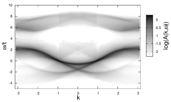
Figure 7: Density plot of the single-particle spectral function of the one-dimensional Hubbard model for $U=4.9t$ and less than half filling ($\rho=0.6$ electrons per site). The spectral function has been calculated on a 90-site open chain using DDMRG with $\eta=0.1t$ and quasi-momenta. The ARPES spectrum corresponds to $\omega<0$ and the inverse ARPES spectrum to $\omega>0$. The spectral function for more than half filling ($\rho=1.4$) is obtained through the transformation $(\omega,k)\rightarrow(-\omega,k+\pi\mod 2\pi)$.

This DDMRG study of the Hubbard model spectral function confirms that dispersive features observed in the ARPES spectrum of the quasi-one-dimensional conductor TTF-TCNQ are the signature of the spin-charge separation in one-dimensional strongly correlated electron systems. The accuracy of the DDMRG results has been demonstrated by a comparison with the exact dispersion of excitations obtained from the Bethe Ansatz solution (as shown in fig. 5 for the half-filled band case) and later confirmed by QMC simulations. [55, 56] Finite-temperature effects and the role of phonons have also been investigated using DMRG methods. [56, 57]

3.3 Electron-phonon systems

Electron-phonon systems are a challenge for DMRG simulations because the Hilbert space of a single phonon site is infinitely large. To deal with this problem a density-matrix renormalization approach has been developed to find an optimal finite-dimensional basis for phonon (or more generally boson) sites. [25] This optimal phonon basis technique can be combined with the Lanczos-vector approach to compute momentum- and energy-resolved dynamical correlation functions in electron-phonon models. However, as the electronic degrees of freedom ae not renormalized using DMRG in this approach but treated exactly, its applicability is restricted to small system sizes. Nevertheless, the method has been demonstrated on the single-particle spectral function and the optical conductivity of the Holstein model at various band fillings. [58] Combined with cluster perturbation theory it allows us to obtain approximate single-particle spectral functions with a higher resolution in $k$-space for infinite systems. [57] This has been used to investigate the effect of phonons of the ARPES spectrum of TTF-TCNQ.

The combination of optimal boson basis and Lanczos algorithm has also been used to investigate the dynamical susceptibility of a dissipative two-state system (a spin-boson model). [59] The obtained results agree with those of QMC simulations.

To calculate the dynamical correlations of large electron-phonon systems one can treat both electron and phonon degrees of freedom with DMRG. [25] For instance, this approach has been used to compute the spectral functions of spin-polarized electrons (spinless fermions) in the Holstein model, which are shown in fig. 5. This approach has also been employed to investigate the single-particle spectral function [56, 51] and the linear optical absorption [50] in extended Holstein-Hubbard models with up to 20 sites. These studies have shown that, for model parameters representing the Mott insulator SrCuO₂ or the organic conductor TTF-TCNQ, the electron-phonon coupling does not influence $A(\omega,k)$ over the energy range observed in ARPES experiments.

3.4 Cold gases in optical lattices

One of the first applications of the correction-vector DMRG method has been the calculation of the ac conductivity in the superfluid phase of the one-dimensional Bose-Hubbard model for correlated bosons in a lattice. [60] The advent of ultracold bosonic atom gases in optical lattices has considerably increased the interest in the dynamics of these systems but DMRG calculations for momentum- and energy-resolved dynamical correlation functions remain scarce. Recently, the spectral function $A(\omega,k)$ has been calculated in a two-component one-dimensional Bose-Hubbard model using a correction-vector MPS method, which improves on the correction-vector DMRG method. [61] Although the model considered describes cold atomic gases with two hyperfine species in a quasi-one-dimensional optical lattice, a comparison with experiment is not possible because momentum- and energy-resolved spectral functions can not be measured in cold atomic gases with the presently available techniques. Therefore, for these systems it is currently more interesting to investigate time-resolved quantities using one of the time-dependent DMRG methods.

4 Conclusion

DMRG methods allow us to calculate the momentum- and energy-resolved dynamical correlation functions of low-dimensional correlated systems on large lattices with several hundreds of sites. The accuracy of these DMRG calculations has been demonstrated by numerous comparisons with exact results and numerical data obtained with other methods. The capability and versatility of DMRG methods are illustrated by the broad range of applications summarized in the previous section. The main drawback of this approach is the limitation to one-dimensional systems and quantum impurity systems and to zero temperature. An advantage of the DMRG approach over other numerical techniques is that it allows for the simulation of systems large enough to obtain information on the spectrum in the thermodynamic limit. In summary, DMRG methods provides a powerful and versatile approach for investigating the dynamical properties in low-dimensional strongly correlated quantum systems.

References

- [1] S.R. White, \PRL69,1992,2863.
- [2] S.R. White, \PRB48,1993,10345.
- [3] U. Schollwöck, Rev. Mod. Phys. 77 (2005), 259.
- [4] K. Hallberg, Adv. Phys. 55 (2006), 477.
- [5] I. Peschel, X. Wang, M. Kaulke and K. Hallberg (eds.), Density-Matrix Renormalization, A New Numerical Method in Physics (Springer, Berlin, 1999).
- [6] An comprehensive introduction to DMRG can be found in Computational Many Particle Physics, H. Fehske, R. Schneider and A. Weiße (Eds.), Lecture Notes in Physics 739 (Springer-Verlag, Berlin, Heidelberg, 2008) Part IX.
- [7] I.P. McCulloch, J. Stat. Mech. (2007), P10014.
- [8] I. Peschel and V. Eisler in Computational Many Particle Physics, H. Fehske, R. Schneider and A. Weiße (Eds.), Lecture Notes in Physics 739 (Springer-Verlag, Berlin, Heidelberg, 2008) p. 581.
- [9] R.M. Noack and S.R. Manmana, in Lectures on the Physics of Highly Correlated Electron Systems IX: Ninth Training Course in the Physics of Correlated Electron Systems and High-Tc Superconductors, vol. 789, ed. by A. Avella and F. Mancini (AIP, 2005), pp. 93–163.
- [10] E. Jeckelmann in Computational Many Particle Physics, H. Fehske, R. Schneider and A. Weiße (Eds.), Lecture Notes in Physics 739 (Springer-Verlag, Berlin, Heidelberg, 2008) p. 597.
- [11] H. Kuzmany, Solid-State Spectroscopy (Springer, Berlin, 1998).
- [12] K.A. Hallberg, \PRB52,1995,R9827.
- [13] T.D. Kühner, S.R. White, \PRB60,1999,335.
- [14] E.R. Gagliano and C.A. Balseiro, \PRL59,1987,2999.
- [15] S. Nishimoto, E. Jeckelmann, F. Gebhard and R.M. Noack, \PRB65,2002,165114.
- [16] Z.G. Soos, S. Ramasesha, J. Chem. Phys. 90 (1989), 1067.
- [17] W. Press, S. Teukolsky, W. Vetterling and B. Flannery, Numerical Recipes in C++. The Art of Scientific Computing (Cambridge University Press, Cambridge, 2002).
- [18] S. Ramasesha, J. Comp. Chem. 11 (1990), 545.
- [19] S.K. Pati, S. Ramasesha, Z. Shuai and J.L. Brédas, \PRB59,1999,14827.
- [20] E. Jeckelmann, \PRB66,2002,045114.
- [21] E. Jeckelmann and H. Benthien in Computational Many Particle Physics, H. Fehske, R. Schneider and A. Weiße (Eds.), Lecture Notes in Physics 739 (Springer-Verlag, Berlin, Heidelberg, 2008) p. 621.
- [22] S. Nishimoto and M. Arikawa, Int. J. Mod. Phys. B 21 (2007), 2262.
- [23] E. Jeckelmann, F. Gebhard and F.H.L. Essler, \PRL85,2000,3910.
- [24] F.H.L. Essler, F. Gebhard and E. Jeckelmann, \PRB64,2001,125119.
- [25] E. Jeckelmann and H. Fehske, in Proceedings of the International School of Physics ”Enrico Fermi” - Course CLXI Polarons in Bulk Materials and Systems with Reduced Dimensionality (IOS Press, Amsterdam, 2006), pp. 247–284; Rivista del Nuovo Cimento 30 (2007), 259.
-
[26]
F. Gebhard, E. Jeckelmann, S. Mahlert, S. Nishimoto and R. Noack, Eur. Phys. J. B
36 (2003), 491.
S. Nishimoto, F. Gebhard and E. Jeckelmann, J. Phys.: Condens. Matter 16 (2004), 7063. - [27] S. Nishimoto and E. Jeckelmann, J. Phys. Condens. Matter 16 (2004), 613.
- [28] H. Benthien, Dynamical properties of quasi one-dimensional correlated electron systems, Ph.D. thesis (Philipps-Universität, Marburg, Germany, 2005).
- [29] H. Benthien, F. Gebhard, E. Jeckelmann, \PRL92,2004,256401.
- [30] E. Jeckelmann, \PRB67,2003,075106.
- [31] C. Raas and G.S. Uhrig, Eur. Phys. J. B 45 (2005), 293.
- [32] G. Hager, E. Jeckelmann, H. Fehske and G. Wellein, Journal of Computational Physics 194 (2004), 795.
- [33] U. Schollwöck and S.R. White, in G.G. Batrouni and D. Poilblanc (eds.), Effective models for low-dimensional strongly correlated systems (AIP, Melville, New York, 2006), p. 155, cond-mat/0606018.
- [34] R.M. Noack, S.R. Manmana, S. Wessel and A. Muramatsu in Computational Many Particle Physics, H. Fehske, R. Schneider and A. Weiße (Eds.), Lecture Notes in Physics 739 (Springer-Verlag, Berlin, Heidelberg, 2008) p. 637.
- [35] S.R. White and I. Affleck, \PRB77,2008,134437.
- [36] R.G. Pereira, S.R. White and I. Affleck, \PRL100,2008,027206.
- [37] W. Yu and S. Haas, \PRB63,2000,024423.
- [38] A. Friedrich, A.K. Kolezhuk, I.P. McCulloch and U. Schollwöck, \PRB75,2007,094414.
- [39] K. Okunishi, Y. Akutsu, N. Akutsu and T. Yamamoto, \PRB64,2001,104432.
- [40] S. Nishimoto and Y. Ohta, \PRB68,2003,235114.
- [41] H. Matsueda, T. Tohyama and S. Maekawa, \PRB70,2004,033102.
- [42] H. Matsueda, T. Tohyama and S. Maekawa, \PRB71,2005,153106.
- [43] H. Benthien and E. Jeckelmann, Eur. Phys. J. B 44 (2005), 287.
- [44] C. Raas, G.S. Uhrig and F.B. Anders, \PRB69,2004,041102.
- [45] S. Nishimoto, T. Pruschke and R.M. Noack, J. Phys.: Condens. Matter 18 (2006), 981.
-
[46]
D.J. Garcia, K. Hallberg and M.J. Rozenberg, \PRL93,2004,246403.
D.J. Garcia, E. Miranda, K. Hallberg and M.J. Rozenberg, \PRB75,2007,121102. - [47] M. Karski, C. Raas and G.S. Uhrig, \PRB72,2005,113110; ibid. \andvol77,2008,075116.
- [48] Y.-J. Kim, J.P. Hill, H. Benthien, F.H.L. Essler, E. Jeckelmann, H.S. Choi, T.W. Noh, N. Motoyama, K.M. Kojima, S. Uchida, D. Casa and T. Gog, \PRL92,2004,137402.
- [49] H. Benthien and E. Jeckelmann, \PRB75,2007,205128.
- [50] H. Matsueda, A. Ando, T. Tohyama and S. Maekawa, arXiv:0802.3965v1.
- [51] H. Matsueda, T. Tohyama and S. Maekawa, \PRB74,2006,241103.
- [52] H. Matsueda, N. Bulut, T. Tohyama and S. Maekawa, \PRB72,2005,075136.
- [53] M. Hoinkis, M. Sing, J. Schaefer, M. Klemm, S. Horn, H. Benthien, E. Jeckelmann, T. Saha-Dasgupta, L. Pisani, R. Valenti and R. Claessen, \PRB72,2005,125127.
-
[54]
S. Ejima, F. Gebhard and S. Nishimoto, Physica C 460-462 (2007), 1079.
S. Nishimoto, T. Shirakawa and Y. Ohta, \PRB77,2008,115102. - [55] A. Abendschein and F.F. Assaad, \PRB73,2006,165119.
- [56] N. Bulut, H. Matsueda, T. Tohyama and S. Maekawa, \PRB74,2006,113106.
- [57] W.-Q. Ning, H. Zhao, C.-Q. Wu and H.-Q. Lin, \PRL96,2006,156402.
- [58] C. Zhang, E. Jeckelmann and S.R. White, \PRB60,1999,14092.
- [59] Y. Nishiyama, Eur. Phys. J. B 12 (1999), 547.
- [60] T.D. Kühner, S.R. White and H. Monien, \PRB61,2000,12474.
- [61] A. Kleine, C. Kollath, I.P. McCulloch, T. Giamarchi and U. Scholwöck, New Journal of Physics 10 (2008), 045025.