Colloidal electrophoresis: Scaling analysis, Green–Kubo relation, and numerical results

Abstract

We consider electrophoresis of a single charged colloidal particle in a finite box with periodic boundary conditions, where added counterions and salt ions ensure charge neutrality. A systematic rescaling of the electrokinetic equations allows us to identify a minimum set of suitable dimensionless parameters, which, within this theoretical framework, determine the reduced electrophoretic mobility. It turns out that the salt–free case can, on the Mean Field level, be described in terms of just three parameters. A fourth parameter, which had previously been identified on the basis of straightforward dimensional analysis, can only be important beyond Mean Field. More complicated behavior is expected to arise when further ionic species are added. However, for a certain parameter regime, we can demonstrate that the salt-free case can be mapped onto a corresponding system containing additional salt. The Green–Kubo formula for the electrophoretic mobility is derived, and its usefulness demonstrated by simulation data. Finally, we report on finite–element solutions of the electrokinetic equations, using the commercial software package COMSOL.

1 Introduction

The behavior of charge–stabilized colloidal dispersions in external electric fields is a classical topic of colloid physics [1]. Quantitative theoretical understanding is still incomplete today, although substantial progress has been achieved over the decades [2, 3, 4, 5, 6, 7, 8, 9]. The difficulty lies in the complicated many–body nature of the problem, and hence only limiting cases are well understood. Beyond the physics of the “standard electrokinetic model” [6], which is essentially just a single–particle Mean Field theory (see below), which nevertheless does describe a quite broad range of phenomena, current research focuses mainly on situations where this model is not applicable, or at least its applicability is not obvious. These include cases where non–Mean Field effects are important, i. e. higher valency or non–negligible size of the ions [7, 8, 10], or where the single–colloid picture is expected to break down, due to overlapping ionic clouds (or insufficient amount of screening by salt) [9]. This latter issue has also triggered detailed experiments [11, 12, 13, 14, 15] which measured the electrophoretic mobility in the low–salt regime. Furthermore, the problem has recently been studied by computer simulations [16, 17, 18, 19, 20, 21]. The investigations of Ref. [21] were specifically targeted at the low–salt limit. The purpose of the present paper is to provide some more detailed theoretical and numerical background material which had to be omitted in Ref. [21]. We will start in Sec. 2 with a brief review of the simplest limiting cases of electrophoresis, followed by a summary of the observations made in Ref. [21]. The new material is then found in Secs. 3–5 (briefly outlined at the end of Sec. 2), while we conclude in Sec. 6.

2 Background: Review of limiting cases, and previous simulation results

2.1 Single colloid without salt

The simplest case of colloidal electrophoresis is obviously a single charged sphere of radius $R$ and charge $Ze$ ($e$ denotes the positive elementary charge, and we assume $Z>0$), immersed in a solvent of viscosity $\eta$ and dielectric constant $\epsilon$. Assuming zero salt concentration, and zero colloidal volume fraction $\Phi$, the drift velocity $\vec{v}$ which results as a response to an external electric field $\vec{E}$ is just given by the Stokes formula,

$$6\pi\eta R\vec{v}=Ze\vec{E}.$$ (1)

This is the so–called Hückel limit [1, 3]. The electrophoretic mobility $\mu$ of the colloidal sphere, defined via

$$\vec{v}=\mu\vec{E},$$ (2)

is hence given by

$$\mu=\frac{Ze}{6\pi\eta R}.$$ (3)

We now introduce the zeta potential as the electrostatic potential at the colloid surface (with the understanding that it vanishes infinitely far away from the colloid):

$$\zeta=\frac{Ze}{4\pi\epsilon R}.$$ (4)

This allows us to re–write (3) as

$$\mu=\frac{2}{3}\frac{\epsilon}{\eta}\zeta.$$ (5)

Based upon the thermal energy $k_{B}T$ as typical energy scale ($k_{B}$ denotes Boltzmann’s constant and $T$ the absolute temperature), we can introduce the dimensionless (reduced) zeta potential as

$$\zeta_{red}=\frac{e\zeta}{k_{B}T}.$$ (6)

On the other hand, the thermal energy, combined with electrostatics, provides a typical length scale, the Bjerrum length

$$l_{B}=\frac{e^{2}}{4\pi\epsilon k_{B}T},$$ (7)

which is nothing but the distance between two elementary charges such that their electrostatic energy is just $k_{B}T$. This can be combined with the Stokes formula to define a useful mobility scale for electrokinetic phenomena:

$$\mu_{0}=\frac{e}{6\pi\eta l_{B}}.$$ (8)

Defining the reduced mobility as

$$\mu_{red}=\frac{\mu}{\mu_{0}},$$ (9)

one sees that in the Hückel limit one simply has

$$\mu_{red}=\zeta_{red}.$$ (10)

2.2 Zeta potential vs. reduced charge

In a more general context, the electrostatic potential at the surface of the colloid will of course no longer be given by (4). It will rather be diminished, as a result of the influence of the other charges. In order to clearly distinguish between the concepts of charge and potential, we will call

$$\tilde{Z}=\frac{Ze}{4\pi\epsilon R}\frac{e}{k_{B}T}=Z\frac{l_{B}}{R}$$ (11)

the reduced (re–parametrized) charge (regardless of the physical situation), while the symbols $\zeta$ and $\zeta_{red}$ are reserved for the actual value of the surface electrostatic potential and its dimensionless counterpart. In the Hückel limit (and only in this limit), $\zeta_{red}$ and $\tilde{Z}$ coincide.

2.3 Screening

An important aspect of electrophoresis is the screening of not only electrostatic, but also hydrodynamic interactions. As soon as one considers a system at a finite concentration, one has to take into account that it must be charge–neutral, at least on sufficiently large length scales: The charges (colloid charges plus ion charges) that are contained in a sub–volume of linear dimension substantially larger than the colloid–colloid correlation length must add up to zero. The same is true (with arbitrary precision) in a computer simulation if one considers the simulation box as a whole (independently of the value of any correlation length).

Now, the basic mechanism of hydrodynamic screening is the fact that the external electric field generates electric currents in both directions, which in turn generate hydrodynamic flows in both directions. In leading order, however, these flows cancel, since the total net force acting on the system (or sub–volume) is exactly zero. As a result, the flow around a moving charged colloid will not decay like $1/r$ (which would hold in the case of sedimentation, where the system responds to a gravitational field and the net force does not vanish), but much faster, $\sim 1/r^{3}$ [22]. The consequence is, on the one hand, that finite size effects in computer simulations are much less severe than in similar studies of sedimentation [10], and, on the other hand, that a single–particle picture will apply whenever the electrostatic interactions are sufficiently screened, as a result of high salt concentration. Indeed, it is well–known that in the high–salt limit the screening of electrostatics [1] is governed by the Debye length $l_{D}=\kappa^{-1}$, where the screening parameter $\kappa$ is proportional to the square root of the salt concentration $c_{s}$:

$$\kappa^{2}=4\pi l_{B}c_{s}.$$ (12)

To be precise, (12) assumes monovalent salt ions, and $c_{s}$ denotes the total number of salt ions per unit volume (such that the number of ion pairs per unit volume is given by $c_{s}/2$). Now, under conditions where $l_{D}$ is substantially smaller than the typical colloidal interparticle separation, it is clear that most of the space between the colloids is charge–neutral. Consequently, these regions are also force–free. In other words, in these regions there is no net flow, and all the hydrodynamic shear gradients and viscous dissipation processes are confined to the Debye layer as well. In this situation, one obviously can treat the problem in terms of a single–particle picture. However, even the problem of a single sphere surrounded by a charge cloud, with boundary condition of vanishing electrostatic potential, and finite salt concentration, for $r\to\infty$, can in general be solved only numerically. This is the so–called “standard electrokinetic model” [6]. The reason for the mathematical difficulties is the non–linearity of the underlying Poisson–Boltzmann equation, which determines the ionic cloud structure.

2.4 Smoluchowski limit

A simple analytic solution is however possible in the limit of very high salt concentration such that $l_{D}\ll R$. Here the geometry is essentially planar, and one obtains the so–called Smoluchowski limit [1]:

$$\mu=\frac{\epsilon}{\eta}\zeta;$$ (13)

however, here the zeta potential is tiny, and in terms of the reduced charge one has

$$\mu_{red}=\frac{3}{2}\tilde{Z}\left(\kappa R\right)^{-1}.$$ (14)

In the limit of infinitely strong screening ($\kappa\to\infty$), the salt completely shields the electric field from the particle, and correspondingly the mobility tends to zero. Of course, this is only a mathematical limit, which can never be reached in practice, since at a critical salt concentration the system of small ions will crystallize. Beyond this critical concentration the liquid–state Smoluchowski formula cannot work.

2.5 Simulations of the low–salt case

While the case of high salt concentration can thus be considered as reasonably well understood (albeit in general only within the framework of numerics), a completely different situation arises when there is only little salt in the solution, or even none at all. In this case the ionic clouds are mainly formed by the counterions, and these will in general overlap. All the standard screening concepts, which are based upon assuming a decay of the electrostatic potential and of the charge density, on a length scale smaller than the colloid–colloid separation, are no longer expected to work. Nevertheless, namely due to the weak screening, some simplifying assumptions can still be made for suspensions of strongly charged colloids. As the colloids in this regime strongly repel each other, they are usually well ordered so that their minimal separation amounts to the mean interparticle distance $d\sim R\Phi^{-1/3}$. Thus, the screening at $r<d$ will be exclusively due to counterions and the phenomena that happen on this length scale will be governed by the mean counterion concentration. These ideas proved to be useful for describing static structure and colloidal interactions at low salt [23].

We have studied this case by computer simulations. In essence, our method is Molecular Dynamics (MD) for the charged colloid, the explicit (counter or salt) ions, and the solvent. However, for computational efficiency the latter is replaced by a lattice Boltzmann (LB) system which is coupled to the particles by a Stokes friction coefficient. This method, which has been designed as an efficient and easy way of simulating systems with hydrodynamic interactions, has been described in Refs. [24, 25], and is discussed in detail in a forthcoming review article [26]. Langevin noise is added to both the particles and the LB system to keep the temperature constant. The colloid is modeled as a “raspberry” [19, 20], i. e. a large central particle with a wrapping consisting of a tether of small particles. The most important results of this study have been communicated in Ref. [21], and can be summarized as follows:

(i) $\mu_{red}$ is a dimensionless quantity, and hence can only depend on dimensionless parameters of the system. As a starting point, we have made no further theoretical assumptions. In the salt–free case, we can then identify four such parameters $p_{1},\ldots,p_{4}$, which we choose in such a way that two of them resemble most closely those quantities which have proven useful in the “salty” case: these are $p_{1}=\kappa R$ and $p_{2}=\tilde{Z}$ (cf. (10) and (14)). In the present case, however, $\kappa$ is not calculated from the salt concentration, but rather from the counterion concentration:

$$\kappa^{2}=4\pi l_{B}c,$$ (15)

with

$$c=\frac{NZ}{V}=Z\frac{3}{4\pi R^{3}}\Phi,$$ (16)

where $V$ is the system volume, and $N$ the number of simulated colloids. Obviously, (15) and (16) imply the relation

$$\left(\kappa R\right)^{2}=3\tilde{Z}\Phi;$$ (17)

in other words, $\kappa R$ is nothing but a re–parametrized volume fraction. It should be emphasized that due to assumed strong charge asymmetry between the colloids and the counterions, which both constitute the screening medium, the resulting charge distribution is strongly inhomogeneous and the standard Debye screening concept cannot be implied. The remaining two scaling variables are $p_{3}=l_{B}/a$ and $p_{4}=l_{B}/R$, where $a$ is the counterion radius.

(ii) For a reasonable choice of parameters ($l_{B}/R$ not too large, and $l_{B}/a$ of order unity, as is typical for ions in water) the dependence on $p_{3}$ and $p_{4}$ can be ignored.

(iii) In terms of $\tilde{Z}$ and $\kappa R$, quite good agreement can be achieved with experiments, provided $Z$ is replaced by an effective charge, calculated from charge renormalization [23, 27, 28].

(iv) Finite–size effects are weak, and hence one can obtain the data for a certain finite volume fraction by just simulating a single sphere in a suitably chosen finite box.

(v) The effect of added salt is similar to that of increased volume fraction. It turns out that it is possible, within good approximation, to just combine these two effects into one single parameter

$$\bar{\kappa}^{2}=4\pi l_{B}\left(c+c_{s}\right),$$ (18)

which has a certain justification within a simplified linearized Poisson–Boltzmann theory [29].

The purpose of the present paper is to provide a theoretical background for the observations reported in Ref. [21] and derive some essential relations needed for the further analysis of the electrophoresis at finite colloidal concentrations. In particular, we describe our rescaling procedure in more detail. We feel that this will become particularly transparent when done in terms of the electrokinetic equations [1], which can be viewed as the Mean Field description of the system we have simulated — in contrast to the simulation, the counterions are not considered as discrete particles, but rather as concentration fields. Section 3 thus presents these equations, and outlines the rescaling procedure. An important result of this analysis is that the dependence on $p_{4}$ can indeed be ignored on the level of the electrokinetic equations — this parameter therefore describes deviations from Mean Field behavior, if there are any. Section 4 discusses the problem of linear response, i. e. how to check that the non–equilibrium simulations employ a sufficiently weak external field. We have solved this by comparing the results with control calculations in strict thermal equilibrium, where the mobility was calculated by Green–Kubo integration. As far as we know, this formula has not yet been presented in the literature, and we will derive it here. Finally, in Sec. 5 we present some data which we have obtained by direct numerical solution of the electrokinetic equations, using the commercial finite element package COMSOL 3.3.

3 Rescaling of the electrokinetic equations

In the stationary state, the electrokinetic equations are given by

$$\nabla\cdot\vec{v}=0,$$ (19)

$$-\nabla p+\eta\nabla^{2}\vec{v}-e(\nabla\Psi)\sum_{i}z_{i}c_{i}=0,$$ (20)

$$\nabla\cdot\left(-D_{i}\nabla c_{i}-\frac{D_{i}}{k_{B}T}ez_{i}(\nabla\Psi)c_{i}+\vec{v}c_{i}\right)=0,$$ (21)

$$\nabla^{2}\Psi+\frac{1}{\epsilon}e\sum_{i}z_{i}c_{i}=0.$$ (22)

Equation (19) is the incompressibility condition for the velocity field $\vec{v}$, while (20) is the Stokes equation for zero Reynolds number flow, where the forces resulting from the hydrostatic pressure $p$ and the viscous dissipation are balanced against the electric force. Here, $\Psi$ denotes the electrostatic potential, while $c_{i}$ is the concentration (number of particles per unit volume) of the $i$th ionic species. We will adopt the convention that $i=0$ corresponds to the counterions, while $i\geq 1$ denotes various types of salt ions. Each ion of species $i$ carries a charge $z_{i}e$. Hence, the total charge density is given by $e\sum_{i}z_{i}c_{i}$; this term appears also in the Poisson equation for the electrostatic potential, (22), where the boundary conditions for $\Psi$ implicitly define the external driving field. Finally, (21) is the so–called Nernst–Planck equation (convection–diffusion equation) which describes the mass conservation of ionic species $i$. Here $D_{i}$ denotes the collective diffusion coefficient of species $i$, while $D_{i}/(k_{B}T)$ is (via the Einstein relation) the corresponding ionic mobility. The ionic current consists of three contributions: the diffusion current, the drift relative to the surrounding solvent, induced by the electric force density $-ez_{i}c_{i}\nabla\Psi$, and finally the convective current induced by the motion of the fluid.

We now introduce

$$M_{i}=\int d^{3}\vec{r}\,c_{i},$$ (23)

the number of ions of species $i$ in the solution, where the integration extends over the finite volume $V$ of the system. Obviously, the counterions just compensate the colloid charge, and hence we have

$$-z_{0}M_{0}=Z;$$ (24)

note that $z_{0}<0$, and we consider only a single colloid in the volume. Similarly, the charges of the salt ions compensate each other, and hence

$$\sum_{i\geq 1}z_{i}M_{i}=0.$$ (25)

In the case without external driving, we have $\vec{v}=0$, and the Stokes equation reduces to an equation which determines the pressure. The Nernst–Planck equation, together with the Poisson equation, then just becomes the Poisson–Boltzmann equation:

$$\nabla\ln c_{i}+z_{i}\nabla\tilde{\Psi}=0,$$ (26)

$$\nabla^{2}\tilde{\Psi}+4\pi l_{B}\sum_{i}z_{i}c_{i}=0,$$ (27)

where we have introduced the abbreviation

$$\tilde{\Psi}=\frac{e\Psi}{k_{B}T}.$$ (28)

In accordance with Ref. [29] and (18), we introduce the parameter

$$\bar{\kappa}^{2}=4\pi l_{B}\frac{\sum_{j}z_{j}^{2}M_{j}}{V},$$ (29)

where however no direct connection to a linearized Poisson–Boltzmann equation is implied. We now use $\bar{\kappa}^{-1}$ as our elementary unit of length and write

$$\nabla=\bar{\kappa}\tilde{\nabla},$$ (30)

which transforms the Poisson equation into a fully non-dimensional form:

$$\tilde{\nabla}^{2}\tilde{\Psi}+\sum_{i}z_{i}\tilde{c}_{i}=0,$$ (31)

where non-dimensional concentrations $\tilde{c}_{i}$ are introduced via

$$c_{i}=\frac{\bar{\kappa}^{2}}{4\pi l_{B}}\tilde{c}_{i}=\frac{\sum_{j}z_{j}^{2}M_{j}}{V}\,\tilde{c}_{i}.$$ (32)

In these scaled variables, the condition of mass conservation of species $i$ is given by

$$\frac{1}{V}\int d^{3}\vec{r}\,\tilde{c}_{i}=\frac{M_{i}}{\sum_{j}z_{j}^{2}M_{j}}=f_{i}$$ (33)

(this equation defines the parameters $f_{i}$), where

$$\sum_{i}z_{i}^{2}f_{i}=1.$$ (34)

$\bar{\kappa}$ as a length unit also defines a dimensionless electric field via

$$\tilde{\vec{E}}=-\tilde{\nabla}\tilde{\Psi}=\frac{e}{\bar{\kappa}k_{B}T}\vec{E},$$ (35)

and a dimensionless velocity $\tilde{v}$ by requiring that the relation $v=\mu E$ transforms into $\tilde{v}=\mu_{red}\tilde{E}$:

$$\vec{v}=\frac{\bar{\kappa}k_{B}T}{6\pi\eta l_{B}}\tilde{\vec{v}}.$$ (36)

The diffusion coefficients $D_{i}$ can be mapped onto length scales $a_{i}$ via a Stokes formula:

$$D_{i}=\frac{k_{B}T}{6\pi\eta a_{i}},$$ (37)

where $a_{i}$ is expected to be similar to the ion radius. Nevertheless, it should be emphasized that the diffusion coefficient $D_{i}$ is a collective diffusion coefficient, not a tracer diffusion coefficient. With these rescalings, the Nernst–Planck equation reads

$$\tilde{\nabla}\cdot\left(-\frac{l_{B}}{a_{i}}\tilde{\nabla}\tilde{c}_{i}-\frac{l_{B}}{a_{i}}z_{i}(\tilde{\nabla}\tilde{\Psi})\tilde{c}_{i}+\tilde{\vec{v}}\tilde{c}_{i}\right)=0.$$ (38)

Finally, we introduce a dimensionless pressure via

$$p=\frac{\bar{\kappa}^{2}k_{B}T}{4\pi l_{B}}\tilde{p},$$ (39)

to re–write the Stokes equation in dimensionless form

$$\tilde{\nabla}\cdot\tilde{\vec{v}}=0,$$ (40)

$$-\tilde{\nabla}\tilde{p}+\frac{2}{3}\tilde{\nabla}^{2}\tilde{\vec{v}}-(\tilde{\nabla}\tilde{\Psi})\sum_{i}z_{i}\tilde{c}_{i}=0.$$ (41)

Let us collect the final set of non–dimensionalized equations:

$$\tilde{\nabla}\cdot\tilde{\vec{v}}=0,$$ (42)

$$-\tilde{\nabla}\tilde{p}+\frac{2}{3}\tilde{\nabla}^{2}\tilde{\vec{v}}-(\tilde{\nabla}\tilde{\Psi})\sum_{i}z_{i}\tilde{c}_{i}=0,$$ (43)

$$\tilde{\nabla}\cdot\left(-\frac{l_{B}}{a_{i}}\tilde{\nabla}\tilde{c}_{i}-\frac{l_{B}}{a_{i}}z_{i}(\tilde{\nabla}\tilde{\Psi})\tilde{c}_{i}+\tilde{\vec{v}}\tilde{c}_{i}\right)=0,$$ (44)

$$\tilde{\nabla}^{2}\tilde{\Psi}+\sum_{i}z_{i}\tilde{c}_{i}=0.$$ (45)

One sees that the only dimensionless parameters which remain in the equations are the ratios $l_{B}/a_{i}$ and the charges $z_{i}$. Therefore, in order to fully characterize the problem, one needs to specify three parameters per ionic species ($l_{B}/a_{i}$, $z_{i}$, and $f_{i}$), plus the parameters which pertain to the boundary conditions: The dimensionless colloid radius $\bar{\kappa}R$, the dimensionless box size $\bar{\kappa}L$ (note that we assume a cubic box with periodic boundary conditions), and the non–dimensionalized charge density at the colloid surface. For the latter, we note that in conventional units the surface charge density is given by

$$\sigma=\frac{Ze}{4\pi R^{2}},$$ (46)

and that an electric field oriented perpendicular to the surface will jump by a value $\sigma/\epsilon$. The jump in $\tilde{E}$ is therefore given by $\tilde{\sigma}=e\sigma/(\bar{\kappa}\epsilon k_{B}T)$, i. e.

$$\tilde{\sigma}=\frac{\tilde{Z}}{\bar{\kappa}R}.$$ (47)

Furthermore, (17) is straightforwardly generalized in the multi–ion case to

$$\Phi=\frac{-z_{0}f_{0}}{3\tilde{Z}}\left(\bar{\kappa}R\right)^{2};$$ (48)

this means that specification of $f_{0}$, $\tilde{Z}$, and $\bar{\kappa}R$ is enough to know $\bar{\kappa}L$.

We can thus summarize: In the case of zero salt and monovalent counterions, the reduced mobility should be a function of just the three parameters $p_{1}=\bar{\kappa}R$, $p_{2}=\tilde{Z}$, and $p_{3}=l_{B}/a$. This result should be contrasted with straightforward dimensional analysis, which was the basis of the treatment in Ref. [21]. Here one does not assume the validity of the electrokinetic equations, i. e. the assumption that the ionic cloud can be treated as a continuum field is not made. Rather, one starts from the observation that the problem is fully characterized by the seven parameters $k_{B}T$, $\eta$, $L$, $Z$, $R$, $l_{B}$, and $a$. We then replace $\eta$ by $\mu_{0}$ (see (8)), $L$ by $\bar{\kappa}$ (see (29)), $Z$ by $\tilde{Z}$ (see (11)), and $a$ by $l_{B}/a$. This results in a new but equivalent set of parameters $k_{B}T$, $\mu_{0}$, $\bar{\kappa}$, $\tilde{Z}$, $R$, $l_{B}$, and $l_{B}/a$. Finally, we replace $l_{B}$ by $l_{B}/R$ and then $R$ by $\bar{\kappa}R$ to find the parameter set $k_{B}T$, $\mu_{0}$, $\bar{\kappa}$, $\tilde{Z}$, $\bar{\kappa}R$, $l_{B}/R$ and $l_{B}/a$. We are thus left with seven parameters, of which $k_{B}T$, $\mu_{0}$, and $\bar{\kappa}$ are needed to define the fundamental units of energy, time, and length, respectively. Since $\mu_{red}$ is a dimensionless quantity, it must be a function of the remaining four dimensionless parameters, which are $p_{1}=\bar{\kappa}R$, $p_{2}=\tilde{Z}$, $p_{3}=l_{B}/a$, and $p_{4}=l_{B}/R$. Since $p_{1}$, $p_{2}$ and $p_{3}$ have also been identified on the basis of Mean Field theory (i. e. the electrokinetic equations), we can only conclude that any non–trivial dependence on $p_{4}$ must be the result of deviations from Mean Field theory, i. e. (most likely) ion correlation effects. As a matter of fact, the successful comparison between simulation and experimental data for $\mu_{red}$ that was done in Ref. [21] exclusively focused on the dependence on $p_{1}$ and $p_{2}$. The justification for this procedure is that (i) $p_{3}$ is of order unity both in simulation and experiment, and that (ii) this implies a moderate strength of electrostatics. This means that ion correlation effects are expected to be weak, which in turn means a rather weak dependence on $p_{4}$, and adequacy of a description in terms of the electrokinetic equations.

In the case of added salt, there are further parameters which enter the problem; however, in the degenerate case, which was simulated in Ref. [21] and where all ion types have the same properties — i. e. all ions are monovalent, and have all the same mobility or $l_{B}/a$ — there are effectively only two ion types (the positive and negative ones), and the only additional scaling variable which enters is $f_{0}$, which specifies the fraction of counterions relative to the salt ions. Apparently, $\mu_{red}$ is only weakly dependent on $f_{0}$ over a wide parameter range [21].

In the case of finite salt concentration, we can consider the limit $f_{0}\to 0$, which implies $\Phi\to 0$ or $L\to\infty$. In this case, the present formulation converges towards the situation studied in the “standard electrokinetic model” [6]. In the case of zero salt, it is not possible to perform the limit $f_{0}\to 0$ within our rescaled formulation, since then $\bar{\kappa}^{-1}\to\infty$, and this is not suitable for a length unit. However, the physics of just a free colloid is anyways trivial (see Sec. 1).

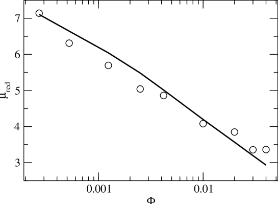
Figure 1: Reduced electrophoretic mobility of the colloidal particle, as a function of the colloid volume fraction $\Phi$. The colloid charge is $Z=20$. The other parameters (in our simulational Lennard–Jones units) are: $\eta=2.55$, $k_{B}T=1$, $R=3$ (friction radius of the “raspberry”, see text), $l_{B}=1.3$, while the coupling of the small particles to the lattice Boltzmann fluid is characterized by a friction constant $\Gamma=20$. For further details on the model, see Refs. [19, 20]. The data points are simulation results. The solid curve is the Hückel formula prediction according to (49).

Figure 1 demonstrates again the general finding that salt–free systems can, within reasonable approximation, be mapped onto the corresponding “salty” system with the same $\tilde{Z}$ and $\bar{\kappa}R$. For a dispersion with charge $Z=20$, we compare the simulation data for $\mu_{red}$, as a function of colloid volume fraction $\Phi$, with the theoretical prediction that results from this mapping. Since it turns out that in the simulated regime of volume fractions $\bar{\kappa}R<1$, it is reasonable to assume that the Hückel formula [1] holds:

$$\mu_{red}=\frac{\tilde{Z}_{\rm eff}}{1+\bar{\kappa}R}=\frac{\tilde{Z}_{\rm eff}}{1+(3\tilde{Z}_{\rm eff}\Phi)^{1/2}}.$$ (49)

Here the factor $(1+\bar{\kappa}R)^{-1}$ takes into account the reduction of the surface potential, within the Debye–Hückel approximation, while $Z_{\rm eff}$ was calculated via the charge renormalization procedure by Alexander et al. [27], based upon the Poisson-Boltzmann cell model. A complication arises from the fact that our “raspberry model” effectively defines two radii: On the one hand, the particles on the surface tether have a distance $R_{1}$ (here: $R_{1}=3$ in our Lennard–Jones units) from the colloid center. Since the tethered particles are those that couple frictionally to the lattice Boltzmann fluid, this is the hydrodynamic radius of the sphere. On the other hand, the minimum distance between the ions and the colloid center is one ion diameter larger, due to the repulsive interaction between tether particles and ions. This defines $R_{2}=4$. It therefore makes sense to calculate the volume fraction and the $\bar{\kappa}R$ parameter on the basis of $R_{2}$, and to also use it in the charge renormalization procedure. However, in the transformation from $Z_{\rm eff}$ to $\tilde{Z}_{\rm eff}=Z_{\rm eff}l_{B}/R$, we used $R_{1}$, in order to obtain the correct Stokes radius in the limit $\bar{\kappa}\to 0$. This procedure yields good agreement between simulation and theory, as seen from Figure 1. For the simulated $\Phi$ values, $Z_{\rm eff}$ varies between $16.2$ and $18.4$.

4 Linear response

In the present section, we will derive the Green–Kubo formula for the electrophoretic mobility, which allows us to determine $\mu$ from pure equilibrium simulations. To our knowledge, the formula has so far not been presented explicitly in the literature; however, the derivation is very straightforward within the framework of standard linear response theory. We follow the approach of Ref. [30], which we find particularly transparent.

Starting point is the Hamiltonian

$${\cal H}(\Gamma,t)={\cal H}_{0}(\Gamma)+{\cal H}^{\prime}(\Gamma,t)={\cal H}_{0}(\Gamma)-f(t)B(\Gamma),$$ (50)

where ${\cal H}_{0}$ describes the unperturbed system, and $f(t)$ is a weak external time–dependent field, which couples linearly to a dynamical variable $B$. $\Gamma$ denotes the phase–space variable. We are interested in the dynamic linear response of a variable $A$. The time dependence of the mean value of $A$, $\overline{A(t)}$, must, for reasons of linearity and time translational invariance, have the form

$$\overline{A(t)}=\left<A\right>+\int_{0}^{\infty}d\tau\chi_{AB}(\tau)f(t-\tau),$$ (51)

where $\left<\ldots\right>$ denotes the thermal average in the absence of perturbations. The dynamic susceptibility $\chi_{AB}$ is defined in such a way that it is zero for negative arguments; this permits extension of the integration range in (51) to $(-\infty,+\infty)$.

For the special case that $f(t)$ is a constant $f_{0}$ for $-\infty<t<0$, and zero from then on, one has, for $t>0$,

$$\overline{A(t)}=\left<A\right>+f_{0}\int_{t}^{\infty}d\tau\chi_{AB}(\tau),$$ (52)

or

$$\frac{d}{dt}\overline{A(t)}=-f_{0}\chi_{AB}(t).$$ (53)

On the other hand, the statistical–mechanical expression for $\overline{A(t)}$ in such a “switch–off experiment” is

$$\overline{A(t)}=\frac{\int d\Gamma\exp\left(-\beta{\cal H}_{0}+\beta f_{0}B\right)A(t)}{\int d\Gamma\exp\left(-\beta{\cal H}_{0}+\beta f_{0}B\right)},$$ (54)

where $\beta=1/(k_{B}T)$, $A(t)$ denotes the time evolution of $A$ under the influence of ${\cal H}_{0}$ only, and the Boltzmann factor describes the averaging over the initial conditions, which are distributed according to the perturbed Hamiltonian. Linearizing this expression with respect to $f_{0}$ for weak perturbations yields

$$\overline{A(t)}=f_{0}\beta\left(\left<B(0)A(t)\right>-\left<B\right>\left<A\right>\right)$$ (55)

or

$$\frac{d}{dt}\overline{A(t)}=f_{0}\beta\left<B(0)\dot{A}(t)\right>.$$ (56)

Comparing this with (53) yields the correlation–function expression for the dynamic susceptibility:

$$\chi_{AB}(t)=-\beta\left<B(0)\dot{A}(t)\right>$$ (57)

for $t>0$. Translational invariance with respect to time implies

$$0=\frac{d}{dt}\left<B(t+\tau)A(t)\right>=\left<\dot{B}(t+\tau)A(t)\right>+\left<B(t+\tau)\dot{A}(t)\right>,$$ (58)

from which one concludes, by setting $\tau=-t$, the alternative (and more useful) representation

$$\chi_{AB}(t)=\beta\left<\dot{B}(0)A(t)\right>.$$ (59)

Considering the case that the external perturbation is completely independent of time, and that $\overline{A}$ settles to a constant value, one thus finds from (51) and (59)

$$\overline{A}=\left<A\right>+f_{0}\beta\int_{0}^{\infty}dt\,\left<\dot{B}(0)A(t)\right>.$$ (60)

For the problem of electrophoresis, we consider a set of particles $i$ with charges $z_{i}e$ at positions $\vec{r}_{i}$, in an electric field $\vec{E}=E\hat{e}_{x}$. The perturbation Hamiltonian is thus given by

$${\cal H}^{\prime}=-Ee\sum_{i}z_{i}x_{i},$$ (61)

i. e. $f_{0}=E$ and $B=e\sum_{i}z_{i}x_{i}$. Denoting the velocity of the $i$th particle in $x$ direction with $v_{ix}$, we thus find

$$\dot{B}=e\sum_{i}z_{i}v_{ix}.$$ (62)

On the other hand, we are interested in the velocity response of one particular particle (say, $i=0$), i. e.

$$A=v_{0x},$$ (63)

with $\left<A\right>=0$. This yields directly the desired Green–Kubo formula for the electrophoretic mobility

$$\mu=\frac{1}{3}\frac{e}{k_{B}T}\sum_{i}z_{i}\int_{0}^{\infty}dt\,\left<\vec{v}_{i}(0)\cdot\vec{v}_{0}(t)\right>,$$ (64)

where we have averaged over the three spatial directions. It should be noticed that the formula involves a mixed correlation between the test particle and all charges, in contrast to the tracer diffusion coefficient, which contains only the autocorrelation of the test particle, and the electric conductivity, which involves the autocorrelation of the collective current.

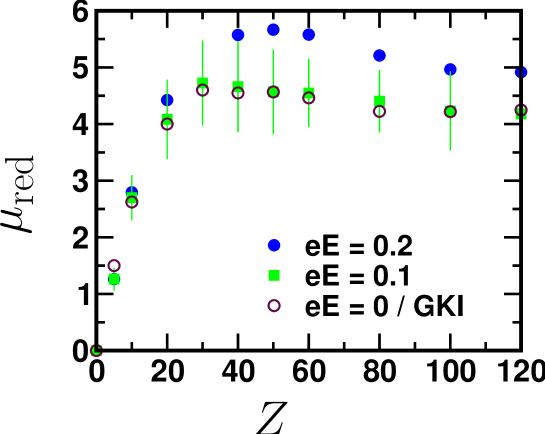
Figure 2: Reduced electrophoretic mobility of the colloidal particle, as a function of its charge $Z$. No salt is added, and, apart from the central colloid, the system comprises $Z$ monovalent counterions. The linear box size is $L=30$. The other simulation parameters are the same as those given in Figure 1. The mobility was here defined just as the ratio between drift velocity and electric field. For strong driving field $E$, one observes nonlinear effects, while the results for weak driving agree favorably with the results of Green–Kubo integration (GKI). Note that the driving field is here given in the Lennard–Jones unit system of the simulation. According to (35), constant $E$ does not imply constant $\tilde{E}$, since $\bar{\kappa}$ varies with $Z$.

As an example, we present Figure 2, where the reduced mobility for a salt–free system is plotted as a function of colloidal charge. Comparison with the Green–Kubo integral makes it possible to check whether data obtained under non-equilibrium conditions are still within the linear regime or not. One sees that the mobility first increases with the charge (as one would expect from the physics of the free colloid), but then saturates at a finite value, as a result of condensation of more and more counterions. The nonlinear effects observed for stronger electric fields are mainly due to charge–cloud stripping [20], which increases the effective charge and thus the mobility.

5 Finite element calculations

As a complementary approach to the hybrid MD / LB simulations, we have also done some calculations where we solved the electrokinetic equations directly, using a commercial finite–element software package (COMSOL 3.3). For highly charged systems, where rather fine grids are necessary, this does not work particularly well, since quite generally the software tends to need excessive amounts of memory. We used the same geometry as in the simulations, with the colloidal sphere centered in the cubic box, but confined, for simplicity, the computational domain to just the space outside the colloidal sphere. This is not entirely correct, since, in reality, the electric field also exists inside the sphere, where it takes a non–trivial configuration, as a result of the external driving field oriented in $x$ direction, the deformed charge cloud, and the cubic anisotropy. However, if we assume that we can neglect the latter, and consider the limit of infinitesimal driving, we get an electric field at the colloid surface whose orientation is strictly radial, and whose value is given by Gauss’ law. This corresponds to the specification of Neumann boundary conditions for the normal component of the electric field. On the surface of the box, we specified Neumann boundary conditions as well, where the normal component was set to zero in the planes perpendicular to $y$ and $z$, while on the planes perpendicular to $x$ it was set equal to the driving field. Concentration and flow field were subjected to periodic boundary conditions. The pressure and the electrostatic potential were set to zero at some arbitrary point in the domain, in order to lift the degeneracy of shifting these functions by an arbitrary amount. The Nernst–Planck equation was augmented by a zero–flux condition at the colloid surface, and an integral constraint in order to guarantee charge neutrality (such integral constraints turn out to be computationally particularly cumbersome). The flow velocity at the colloid surface was set to zero, and the particle velocity was finally determined by transforming back into the system’s center–of–mass reference frame. Given the inaccuracies of the boundary conditions, these results should not be viewed as a stringent test of the validity of the Mean Field picture for the simulated system. Nevertheless, the results agree reasonably: Figure 3 shows the reduced mobility as a function of the external driving field, for a situation which corresponds to the parameters of Figure 2 at charge $Z=60$. In the future, we hope to be able to calculate reduced mobilities in the low–salt limit more easily by self–written software; efforts to develop such a program are currently under way.

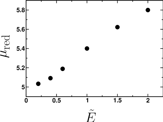
Figure 3: Reduced mobility as a function of electric field $\tilde{E}$, for parameters chosen in accordance with those of Figure 2, for charge $Z=60$. Note that the electric field is given here in reduced units (see (35)), i. e. a value of $\tilde{E}=1$ in the present plot corresponds to $eE\approx 0.2$ in the Lennard–Jones units of Figure 2.

6 Summary

In this paper we developed a theoretical basis for the scaling analysis of the colloidal electrophoresis problem in the case of finite colloidal concentrations. The rescaling procedure and characterization of the dispersion in terms of effective dimensionless parameters, i. e. the reduced colloid charge, and the ratio of screening length and size, allows one to map the numerical results obtained for a single colloid onto experimental data for finite colloidal volume fractions and no added salt. At least for a certain parameter regime, we can also map the salt–free case onto a corresponding system containing additional salt. Moreover, we presented a numerically convenient method of measuring the colloidal electrophoretic mobility based on the Green–Kubo analysis of the equilibrium fluctuations of the charge motions. This allows for pure equilibrium simulations and ensures that one always measures the mobility and ion distributions in the linear response regime. Finally, we gave an example of using a finite-element commercial software package for solving the electrokinetic equations numerically, yielding reasonable agreement with the simulations, and suggesting at least consistency of the Mean Field picture with our simulations.

References

References

- [1] Russel W B, Saville D A and Schowalter W R 1989 Colloidal Dispersions (Cambridge: Cambridge University Press)
- [2] von Smoluchowksi M 1903 Bull. Akad. Sci. Cracovie, Classe Sci. Math. Natur. 1 182
- [3] Hückel E 1924 Physik. Z. 25 204
- [4] Henry D C 1931 Proc. R. Soc. (London) Ser. A 133 106
- [5] Wiersema P H, Loeb A L and Overbeek J T G 1966 J. Colloid Interface Sci. 22 70
- [6] O’Brien R and White L 1978 J. Chem. Soc. Faraday Trans. 74 1607
- [7] Lozada-Cassou M, González-Tovar E and Olivares W 1999 Phys. Rev. E 60 R17
- [8] Lozada-Cassou M and Gonzáles-Tovar E 2001 J. Colloid Interface Sci. 239 285
- [9] Carrique F, Arroyo F J, Jimenez M L and Delgado A V 2003 J. Phys. Chem. B 107 3199
- [10] Tanaka M and Grosberg A Y 2001 J. Chem. Phys. 115 567
- [11] Wette P, Schöpe H J and Palberg T 2002 J. Chem Phys. 116 10981
- [12] Medebach M and Palberg T 2003 J. Chem. Phys. 119 3360
- [13] Medebach M and Palberg T 2004 J. Phys. Condens. Matter 16 5653
- [14] Palberg T, Medebach M, Garbow N, Evers M, Fontecha A B and Reiber H 2004 J. Phys. Condens. Matter 16 S4039
- [15] Medebach M 2005 J. Chem. Phys. 123 104903
- [16] Kim K, Nakayama Y and Yamamoto R 2006 Phys. Rev. Lett. 96 208302
- [17] Chatterji A and Horbach J 2005 J. Chem. Phys. 122 184903
- [18] Chatterji A and Horbach J 2007 J. Chem. Phys. 126 064907
- [19] Lobaskin V and Dünweg B 2004 New J. Phys. 6 54
- [20] Lobaskin V, Dünweg B and Holm C 2004 J. Phys. Condens. Matter 16 S4063
- [21] Lobaskin V, Dünweg B, Medebach M, Palberg T and Holm C 2007 Phys. Rev. Lett. 98 176105
- [22] Long D and Ajdari A 2001 Eur. Phys. J. E 4 29
- [23] Rojas-Ochoa L F, Castaneda-Priego R, Lobaskin V, Stradner A, Scheffold F and Schurtenberger P 2008 Phys. Rev. Lett. 100 178304
- [24] Ahlrichs P and Dünweg B 1998 Int. J. Mod. Phys. C 9 1429
- [25] Ahlrichs P and Dünweg B 1999 J. Chem. Phys. 111 8225
- [26] Dünweg B and Ladd A J C 2008 arXiv:0803.2826v1, submitted to Adv. Polym. Sci.
- [27] Alexander S, Chaikin P M, Grant P, Morales G J, Pincus P and Hone D 1984 J. Chem. Phys. 80 5776
- [28] Belloni L 1998 Colloids and Surfaces A 140 227
- [29] Beresford-Smith B, Chan D Y C and Mitchell D J 1985 J. Colloid Interface Sci. 105 216
- [30] Frenkel D and Smit B 2002 Understanding Molecular Simulation (San Diego: Academic Press)