now at ]Okayama University, Okayama The Belle Collaboration

 
Measurement of $B^{0}\to\pi^{+}\pi^{-}\pi^{+}\pi^{-}$ Decays and Search for $B^{0}\to\rho^{0}\rho^{0}$

Abstract

We report on a search for the decay $B^{0}\to\rho^{0}\rho^{0}$ and other charmless modes with a $\pi^{+}\pi^{-}\pi^{+}\pi^{-}$ final state, including $B^{0}\to\rho^{0}\pi^{+}\pi^{-}$, non-resonant $B^{0}\to 4\pi^{\pm}$, $B^{0}\to\rho^{0}f_{0}(980)$, $B^{0}\to f_{0}(980)f_{0}(980)$ and $B^{0}\to f_{0}(980)\pi^{+}\pi^{-}$. These results are obtained from a data sample containing 657 million $B\overline{B}$ pairs collected with the Belle detector at the KEKB asymmetric-energy $e^{+}e^{-}$ collider. We set an upper limit on $\mathcal{B}(B^{0}\to\rho^{0}\rho^{0})$ of $1.0\times 10^{-6}$ at the 90% confidence level (C.L.). From our $B^{0}\to\rho^{0}\rho^{0}$ measurement and an isospin analysis, we determine the Cabibbo-Kobayashi-Maskawa phase $\phi_{2}$ to be $91.7\pm 14.9$ degrees. We find excesses in $B^{0}\to\rho^{0}\pi^{+}\pi^{-}$ and non-resonant $B^{0}\to 4\pi^{\pm}$ with 1.3$\sigma$ and 2.5$\sigma$ significance, respectively. The corresponding branching fractions are less than $12.0\times 10^{-6}$ and $19.3\times 10^{-6}$ at the 90% C.L. In addition, we set 90% C.L. upper limits as follows: $\mathcal{B}(B^{0}\to\rho^{0}f_{0}(980))<0.3\times 10^{-6}$, $\mathcal{B}(B^{0}\to f_{0}(980)f_{0}(980))<0.1\times 10^{-6}$, and $\mathcal{B}(B^{0}\to f_{0}(980)\pi^{+}\pi^{-})<3.8\times 10^{-6}$.

In the Standard Model (SM), $CP$ violation in the weak interaction can be described by an irreducible complex phase in the three-generation Cabibbo-Kobayashi-Maskawa (CKM) quark-mixing matrix 1 . Measurements of the differences between $B$ and $\overline{B}$ meson decays provide an opportunity to determine the elements of the CKM matrix and thus test the SM. One can extract the CKM phase $\phi_{2}\equiv\mathrm{arg}[-(V_{td}V_{tb}^{*})/(V_{ud}V_{ub}^{*})]$ from the time-dependent $CP$ asymmetry for the decay of a neutral $B$ meson via a $b\to u$ process into a $CP$ eigenstate. However, in addition to the $b\to u$ process, there are $b\to d$ penguin transitions that shift the $\phi_{2}$ value by $\delta\phi_{2}$ in the time-dependent $CP$ violating parameter measurement. The shift $\delta\phi_{2}$ can be determined from an isospin analysis 2 of $B\to\pi\pi$ 202 or $B\to\rho\rho$ 203 decays, or from a time-dependent Dalitz plot analysis of $B\to\rho\pi$ 201 decays.

For $B\to\rho\rho$ decays, polarization measurements in $B\to\rho^{+}\rho^{-}$ 203 and $B^{\pm}\to\rho^{\pm}\rho^{0}$ rho0rhop show the dominance of longitudinal polarization, indicating that the final state in $B\to\rho^{+}\rho^{-}$ is very nearly a $CP$ eigenstate. Measurements of the branching fraction, polarization and $CP$-violating parameters in $B^{0}\to\rho^{0}\rho^{0}$ decays complete the isospin triangle. The tree contribution to $B^{0}\to\rho^{0}\rho^{0}$ is color-suppressed, so its branching fraction is expected to be much smaller than that for $B\to\rho^{+}\rho^{-}$ or $B^{\pm}\to\rho^{\pm}\rho^{0}$. This also makes it especially sensitive to the penguin amplitude, and using the $B^{0}\to\rho^{0}\rho^{0}$ branching fraction in an isospin analysis allows one to determine $\phi_{2}$ free of uncertainty from penguin contributions.

Predictions for $B^{0}\to\rho^{0}\rho^{0}$ using perturbative QCD (pQCD) 32 or QCD factorization 13 ; 14 approaches suggest that the branching fraction $\mathcal{B}(B^{0}\to\rho^{0}\rho^{0})$ is at or below $1\times 10^{-6}$, and that its longitudinal polarization fraction $f_{\mathrm{L}}$ is around 0.85. A non-zero branching fraction for $B^{0}\to\rho^{0}\rho^{0}$ has been reported by the BaBar collaboration 11 ; 1100 ; they measured $\mathcal{B}(B^{0}\to\rho^{0}\rho^{0})=(0.92\pm 0.32\pm 0.14)\times 10^{-6}$ with a significance of 3.1 standard deviations ($\sigma$), and a longitudinal polarization fraction, $f_{\mathrm{L}}=0.75^{+0.11}_{-0.14}\pm 0.05$. They do not observe a non-resonant $B^{0}\to 4\pi^{\pm}$ or $B^{0}\to\rho^{0}\pi^{+}\pi^{-}$ contribution. The theoretical prediction for the non-resonant $B^{0}\to 4\pi^{\pm}$ branching fraction is around $1\times 10^{-4}$ 34 . The most recent measurement of this decay was made by the DELPHI collaboration 33 , which sets a 90% C.L. upper limit on the branching fraction of $2.3\times 10^{-4}$.

The data sample used in the analysis reported here contains 657 million $B\overline{B}$ pairs collected with the Belle detector at the KEKB asymmetric-energy $e^{+}e^{-}$ (3.5 and 8 GeV) collider 101 , operating at the $\Upsilon(4S)$ resonance. The Belle detector 102 ; 103 is a large-solid-angle magnetic spectrometer that consists of a silicon vertex detector, a 50-layer central drift chamber (CDC), an array of aerogel threshold Cherenkov counters (ACC), a barrel-like arrangement of time-of-flight scintillation counters (TOF), and an electromagnetic calorimeter comprised of CsI(Tl) crystals (ECL) located inside a superconducting solenoid coil that provides a 1.5 T magnetic field. An iron flux-return located outside of the coil is instrumented to detect $K^{0}_{L}$ mesons and to identify muons. Signal Monte Carlo (MC) is generated with EVTGEN Lange , in which final-state radiation is taken into account with the PHOTOS package 105 , and processed through a full detector simulation program based on GEANT3 Brun .

$B^{0}$ meson candidates are reconstructed from neutral combinations of four charged pions. Charged track candidates are required to have a distance-of-closest-approach to the interaction point (IP) of less than 2 cm in the direction along the the positron beam ($z$-axis) and less than 0.1 cm in the transverse plane; they are also required to have a transverse momentum $p_{T}>0.1$ GeV/$c$ in the laboratory frame. Charged pions are identified using particle identification (PID) information obtained from the CDC ($dE/dx$), the ACC and the TOF. We distinguish charged kaons and pions using a likelihood ratio $\mathcal{R}_{\mathrm{PID}}=\mathcal{L}_{K}/(\mathcal{L}_{K}+\mathcal{L}_{\pi})$, where $\mathcal{L}_{\pi}(\mathcal{L}_{K})$ is the likelihood value for the pion (kaon) hypothesis. We require $\mathcal{R}_{\mathrm{PID}}<0.4$ for the four charged pions. We require that charge tracks have a laboratory momentum in the range [0.5, 4.0] GeV/$c$, and a polar angle in the range $[32.2,127.2]^{\circ}$. For such tracks the pion identification efficiency is 90%, and the kaon misidentification probability is 12%. Charged particles that are positively identified as an electron or a muon are removed.

To veto $B\to D^{(*)}\pi$ and $B\to D_{s}\pi$ backgrounds, we remove candidates that satisfy either of the conditions $|M(h^{\pm}\pi^{\mp}\pi^{\mp})-m_{D_{(s)}}|<13\ \mathrm{MeV}/c^{2}$ or $|M(h^{\pm}\pi^{\mp})-m_{D^{0}}|<13\ \mathrm{MeV}/c^{2}$, where $h^{\pm}$ is either a pion or a kaon, and $m_{D_{(s)}}$ and $m_{D^{0}}$ are the masses of the $D_{(s)}$ and $D^{0}$ mesons, respectively. Furthermore, to reduce the $B^{0}\to a_{1}^{\pm}\pi^{\mp}$ feeddown in the signal region, we require that the pion with the highest momentum have a momentum in the $\Upsilon(4S)$ center-of-mass (CM) frame within the range [1.30, 2.65] GeV/$c$.

The signal event candidates are characterized by two kinematic variables: the beam-energy-constrained mass, $M_{\mathrm{bc}}=\sqrt{E^{2}_{\mathrm{beam}}-P^{2}_{B}}$, and the energy difference, $\Delta E=E_{B}-E_{\mathrm{beam}}$, where $E_{\mathrm{beam}}$ is the run-dependent beam energy, and $P_{B}$ and $E_{B}$ are the momentum and energy of the $B$ candidate in the $\Upsilon(4S)$ CM frame. In $B^{0}\to\rho^{0}\rho^{0}\to(\pi^{+}\pi^{-})(\pi^{+}\pi^{-})$ decays, or other charmless modes with a $\pi^{+}\pi^{-}\pi^{+}\pi^{-}$ final state, the invariant masses $M(\pi^{+}\pi^{-})$ vs. $M(\pi^{+}\pi^{-})$ are used to distinguish different modes. There are two possible combinations for $M(\pi^{+}\pi^{-})$ vs. $M(\pi^{+}\pi^{-})$: $(\pi^{+}_{1}\pi^{-}_{1})(\pi^{+}_{2}\pi^{-}_{2})$ and $(\pi^{+}_{1}\pi^{-}_{2})(\pi^{+}_{2}\pi^{-}_{1})$, where the subscripts label the momentum ordering, i.e. $\pi^{+}_{1}$($\pi^{-}_{1}$) has a higher momentum than $\pi^{+}_{2}$($\pi^{-}_{2}$). Here we consider both $(\pi^{+}_{1}\pi^{-}_{1})(\pi^{+}_{2}\pi^{-}_{2})$ and $(\pi^{+}_{1}\pi^{-}_{2})(\pi^{+}_{2}\pi^{-}_{1})$ combinations and select candidate events if either one of the combined masses lies within the signal window [0.55, 1.7] GeV/$c^{2}$. This signal window is chosen to accept $\rho^{0}\to\pi^{+}\pi^{-}$, $f_{0}(980)\to\pi^{+}\pi^{-}$, and non-resonant modes, and to exclude $K_{s}^{0}\to\pi^{+}\pi^{-}$ and charm meson decays such as $D^{0}\to\pi^{+}\pi^{-}$. If both $(\pi^{+}_{1}\pi^{-}_{1})(\pi^{+}_{2}\pi^{-}_{2})$ and $(\pi^{+}_{1}\pi^{-}_{2})(\pi^{+}_{2}\pi^{-}_{1})$ combinations of a candidate has a $\pi^{+}\pi^{-}$ pair with an invariant mass in the signal window, we select the $(\pi^{+}_{1}\pi^{-}_{2})(\pi^{+}_{2}\pi^{-}_{1})$ combination. According to MC simulation, this criteria selects the correct combination for $\rho^{0}\rho^{0}$ signal decays 98% of the time. For fitting, we symmetrize the $M^{2}(\pi^{+}\pi^{-})$ vs. $M^{2}(\pi^{+}\pi^{-})$ Dalitz plot by plotting the $\pi^{+}_{2}\pi^{-}_{1}$ $(\pi^{+}_{1}\pi^{-}_{2})$ combination against the horizontal axis for events with an even (odd) event identification number, which is the location of the event in the data.

The dominant background comes from continuum $e^{+}e^{-}\to q\bar{q}$ ($q=u,d,c~{}{\rm or}~{}s$) events. To distinguish signal from the jet-like continuum background, we use modified Fox-Wolfram moments 104 , which are combined into a Fisher discriminant. This discriminant is combined with PDFs for the cosine of the $B$ flight direction in the CM frame and the distance in the $z$-axis between two $B$ mesons to form a likelihood ratio $\mathcal{R}=\mathcal{L}_{s}/(\mathcal{L}_{s}+\mathcal{L}_{q\overline{q}})$. Here, $\mathcal{L}_{s}$ ($\mathcal{L}_{q\overline{q}}$) is a likelihood function for signal (continuum) events that is obtained from the signal MC simulation (events in the sideband region $M_{\rm bc}<5.26$ GeV/$c^{2}$). We also use a flavor tagging quality variable $r$ provided by the Belle tagging algorithm 112 that identifies the flavor of the accompanying $B^{0}$ meson in the $\Upsilon(4S)\to B^{0}\overline{B}^{0}$ decay. The variable $r$ ranges from $r=0$ for no flavor discrimination to $r=1$ for unambiguous flavor assignment, and it is used to divide the data sample into six $r$ bins. Since the discrimination between signal and continuum events depends on the $r$-bin, we impose different requirements on $\mathcal{R}$ for each $r$-bin. We determine the $\mathcal{R}$ requirement such that it maximizes a figure-of-merit $N_{s}/\sqrt{N_{s}+N_{q\overline{q}}}$, where $N_{s}$ $(N_{q\overline{q}})$ is the expected number of signal (continuum) events in the signal region. For 22% of the events, there are multiple candidates; for these events we select the candidate with the smallest $\chi^{2}$ value for the $B^{0}$ decay vertex reconstruction. This selects the correct combination 79.6% of the time. The detection efficiency for the signal is calculated by MC to be 9.16% (11.25%) for longitudinal (transverse) polarization. Since longitudinally polarized $B^{0}\to\rho^{0}\rho^{0}$ decays produce low momentum pions from one or both $\rho^{0}$’s, their detection efficiency is lower than that for transversely polarized decays.

Since there are large overlaps between $B^{0}\to\rho^{0}\rho^{0}$ and other signal decay modes in the $M_{1}(\pi^{+}\pi^{-})$ vs. $M_{2}(\pi^{+}\pi^{-})$ distribution, we distinguish these modes by fitting to a large $M_{1}(\pi^{+}\pi^{-})$ vs. $M_{2}(\pi^{+}\pi^{-})$ region. The signal yields are extracted by performing extended unbinned maximum likelihood (ML) fits. In the fits, we use four-dimensional ($M_{\mathrm{bc}}$, $\Delta E$, $M_{1}$, $M_{2}$) information to discriminate among $\rho^{0}\rho^{0}$, $\rho^{0}\pi^{+}\pi^{-}$, non-resonant $4\pi^{\pm}$, $\rho^{0}f_{0}$, $f_{0}f_{0}$ and $f_{0}\pi^{+}\pi^{-}$ final states. We define the likelihood function

$$\mathcal{L}=\exp\biggl{(}-\sum_{j}n_{j}\biggr{)}\prod^{\mathrm{N_{cand}}}_{i=1}\biggl{(}\sum_{j}n_{j}P^{i}_{j}\biggr{)},$$ (1)

where $i$ is the event identifier, $j$ indicates one of the event type categories for signals and backgrounds, $n_{j}$ denotes the yield of the $j$-th category, and $P^{i}_{j}$ is the probability density function (PDF) for the $j$-th category. The PDFs are a product of two smoothed two-dimensional functions: $P^{i}_{j}=P_{j}(M^{i}_{\mathrm{bc}},\Delta E^{i},M^{i}_{1},M^{i}_{2})=p(M^{i}_{\mathrm{bc}},\Delta E^{i})\times p(M^{i}_{1},M^{i}_{2})$.

For the $B$ decay components, the smoothed functions $p_{\mathrm{smoothed}}(M^{i}_{\mathrm{bc}},\Delta E^{i})$ and $p_{\mathrm{smoothed}}(M^{i}_{1},M^{i}_{2})$ are obtained from MC simulations. For the $M_{\mathrm{bc}}$ and $\Delta E$ PDFs, possible differences between real data and the MC modeling are calibrated using a large control sample of $B^{0}\to D^{-}(K^{+}\pi^{-}\pi^{-})\pi^{+}$ decays. The signal mode PDF is divided into two parts: one is correctly reconstructed events and the other is “self-cross-feed” (SCF), in which at least one track from the signal decay is replaced by one from the accompanying $B$ meson decay. We use different PDFs for the correctly reconstructed and SCF events, and fix the SCF fraction to that from the MC simulation in the nominal fit.

For the continuum and charm $B$ decay backgrounds, we use the product of a linear function for $\Delta E$, an ARGUS function 106 for $M_{\mathrm{bc}}$ and a two-dimensional smoothed function for $M_{1}$-$M_{2}$. The parameters of the linear function and ARGUS function for the continuum events are floated in the fit. Other parameters and the shape of the $M_{1}$-$M_{2}$ functions are obtained from MC simulations and fixed in the fit.

For the charmless $B$ decay backgrounds, we use three separate PDFs for $B^{0}\to a_{1}^{\pm}\pi^{\mp}$, $B^{\pm}\to\rho^{\pm}\rho^{0}$ and other charmless $B$ decays; all of the PDFs are obtained from MC simulations. In the fit, we fix the branching fraction of $B^{0}\to a_{1}^{\pm}\pi^{\mp}$ to the published value $(33.2\pm 3.0\pm 3.8)\times 10^{-6}$ 107 . If we float the $B^{0}\to a_{1}^{\pm}\pi^{\mp}$ yield in the fit, the fit result is $\mathcal{B}(B^{0}\to a_{1}^{\pm}\pi^{\mp})=(33.8^{+13.4}_{-13.2})\times 10^{-6}$, which is consistent with the assumed value. We fix the yield of $B^{\pm}\to\rho^{\pm}\rho^{0}$ to that expected based on the world average branching fraction rho0rhop , and we float the yield of other charmless $B$ decays.

Table 1 and Fig. 1 show the fit results and projections of the data onto $\Delta E$, $M_{\mathrm{bc}}$, $M_{1}(\pi^{+}\pi^{-})$ and $M_{2}(\pi^{+}\pi^{-})$ for $B^{0}\to\rho^{0}\rho^{0}$ decay. The statistical significance is defined as $\sqrt{-2\ln(\mathcal{L}_{0}/\mathcal{L}_{\mathrm{max}})}$, where $\mathcal{L}_{0}$ and $\mathcal{L}_{\mathrm{max}}$ are the values of the likelihood function when the signal yield is fixed to zero and allowed to vary, respectively. The 90% C.L. (C.L.) upper limit for the yield $N$ is calculated from the equation

$${{\int_{0}^{N}\mathcal{L}(x)dx}\over{\int_{0}^{\infty}\mathcal{L}(x)dx}}=90\%,$$ (2)

where $x$ corresponds to the number of signal events. We include the systematic uncertainty into the upper limit (UL) by smearing the statistical likelihood function by a bifurcated Gaussian whose width is equal to the total systematic error. The significance including systematic uncertainties is calculated as before, except that we only include the additive systematic errors related to signal yield in the convoluted Gaussian width.

Table 1: Fit results for the decay modes listed in the first column. The signal yields, reconstruction efficiencies (assuming the probability for the sub-decay mode $f_{0}(980)\to\pi^{+}\pi^{-}$ is 100%), significance ($\mathcal{S}$, in units of $\sigma$), branching fractions ($\mathcal{B}$, in units of $10^{-6}$) and the upper limit at the 90% C.L. (UL, in units of $10^{-6}$) are listed. For the yields and branching fractions, the first (second) error is statistical (systematic).

Mode	Yield	Eff.(%)	$\mathcal{S}$	$\mathcal{B}$	UL
$\rho^{0}\rho^{0}$	$24.5^{+23.6+10.1}_{-22.1-16.2}$	9.16	1.0	$0.4\pm 0.4^{+0.2}_{-0.3}$	$<1.0$
$\rho^{0}\pi^{+}\pi^{-}$	$112.5^{+67.4}_{-65.6}\pm 52.3$	2.90	1.3	$5.9^{+3.5}_{-3.4}\pm 2.7$	$<12.0$
$4\pi^{\pm}$	$161.2^{+61.2+27.7}_{-59.4-25.1}$	1.98	2.5	$12.4^{+4.7+2.1}_{-4.6-1.9}$	$<19.3$
$\rho^{0}f_{0}$	$-11.8^{+14.5+4.8}_{-12.9-3.6}$	9.81	$-$	$-$	$<0.3$
$f_{0}f_{0}$	$-7.7^{+4.7}_{-3.5}\pm 3.0$	10.17	$-$	$-$	$<0.1$
$f_{0}\pi^{+}\pi^{-}$	$6.3^{+37.0}_{-34.7}\pm 18.0$	2.98	$-$	$0.3^{+1.9}_{-1.8}\pm 0.9$	$<3.8$

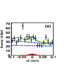
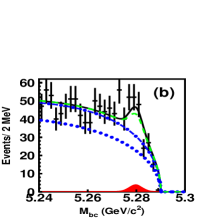
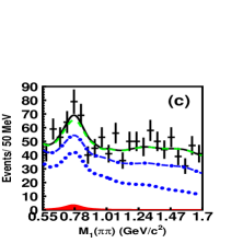
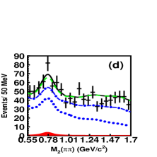
Figure 1: Projections of the four-dimensional fit onto (a) $\Delta E$, (b) $M_{\mathrm{bc}}$, (c) $M_{1}(\pi^{+}\pi^{-})$, and (d) $M_{2}(\pi^{+}\pi^{-})$, for candidates satisfying (except for the variable plotted) the criteria $\Delta E\in[-0.05,\ 0.05]\ \mathrm{GeV}$, $M_{\mathrm{bc}}\in[5.27,\ 5.29]\ \mathrm{GeV}/c^{2}$, and $M_{1,2}(\pi^{+}\pi^{-})\in[0.626,\ 0.926]\ \mathrm{GeV}/c^{2}$. The fit result is shown as the thick solid curve; the solid shaded region represents the $B^{0}\to\rho^{0}\rho^{0}$ signal component. The dotted, dot-dashed and dashed curves represent, respectively, the cumulative background components from continuum processes, $b\to c$ decays, and charmless $B$ backgrounds.

The fractional systematic errors are summarized in Table 2. For the systematic uncertainties due to the fixed branching fractions, we vary the branching fractions of $B^{0}\to a_{1}^{\pm}\pi^{\mp}$ ($33.2\pm 4.8$, in units of $10^{-6}$) 107 and $B^{\pm}\to\rho^{\pm}\rho^{0}$ ($18.2\pm 3.0$) 108 by their $\pm 1\sigma$ errors. The fits are repeated and the differences between the results and the nominal fit values are taken as systematic errors. Systematic uncertainties for the $\Delta E$-$M_{\rm bc}$ PDFs used in the fit are estimated by performing the fits while varying the signal peak positions and resolutions by $\pm 1\sigma$. Systematic uncertainties for the $M_{1}$-$M_{2}$ PDFs are estimated in a similar way. A systematic error for the longitudinal polarization fraction of $B^{0}\to\rho^{0}\rho^{0}$ is obtained by changing the fraction from the nominal value $f_{\mathrm{L}}=1$ to the most extreme alternative value $f_{\mathrm{L}}=0$. According to MC, the signal SCF fractions are 20.4% for $B^{0}\to\rho^{0}\rho^{0}$, 14.2% for $B^{0}\to\rho^{0}\pi^{+}\pi^{-}$, 11.1% for non-resonant $B^{0}\to 4\pi^{\pm}$, 15.0% for $B^{0}\to\rho^{0}f_{0}$, 9.9% for $B^{0}\to f_{0}f_{0}$ and 13.4% for $B^{0}\to f_{0}\pi^{+}\pi^{-}$. We estimate a systematic uncertainty for the signal SCF by varying its fraction by $\pm 50\%$.

An MC study indicates that the fit biases are $+2.4$ events for $B^{0}\to\rho^{0}\rho^{0}$, $+7.2$ events for $B^{0}\to\rho^{0}\pi^{+}\pi^{-}$, $+12.5$ events for non-resonant $B^{0}\to 4\pi^{\pm}$, $+3.6$ events for $B^{0}\to\rho^{0}f_{0}$, $-0.8$ event for $B^{0}\to f_{0}f_{0}$ and $+5.1$ events for $B^{0}\to f_{0}\pi^{+}\pi^{-}$. We find that fit biases occur due to the correlations between the two sets of variables ($\Delta E$, $M_{\rm bc}$) and ($M_{1}$, $M_{2}$), which are not taken into account in our fit. We correct the fit yields for these biases. To take into account possible differences between the MC simulation and data, we take both the magnitude of the bias corrections and the uncertainty in the corrections as systematic errors.

We study the possible interference between $B^{0}\to a_{1}^{\pm}\pi^{\mp}$, $B^{0}\to\rho^{0}\rho^{0}$, $B^{0}\to\rho^{0}\pi^{+}\pi^{-}$ and non-resonant $B^{0}\to 4\pi^{\pm}$ using toy MC. We add a simple interference model to the toy MC generation, which is, for $\rho^{0}\to\pi^{+}\pi^{-}$ decay, modified from a relativistic Breit-Wigner function to

$$\small\Biggl{|}{1\over{m^{2}-m_{0}^{2}+im_{0}\Gamma}}+A\mathrm{e}^{-i\delta}\Biggr{|}^{2}=\ \ \ \ \ \ \ \ \ \ \$$

$$A^{2}+2A\Biggl{[}{{(m^{2}-m_{0}^{2})\cos\delta-\Gamma m_{0}\sin\delta}\over{(m^{2}-m_{0}^{2})^{2}+(\Gamma m_{0})^{2}}}\Biggr{]}$$

$$+{1\over{(m^{2}-m_{0}^{2})^{2}+(\Gamma m_{0})^{2}}},\ \ \ \ \ \ \ \ \ \ \ \ \ \ \ \ \ \ \$$ (3)

where $A$ and $\delta$ are the interfering amplitude and phase, and $m_{0}$ and $\Gamma$ are the $\rho^{0}$ mass and width, respectively. We assume that the interference term due to the amplitudes for $B^{0}\to a_{1}^{\pm}\pi^{\mp}$, $B^{0}\to\rho^{0}\pi^{+}\pi^{-}$ and non-resonant $B^{0}\to 4\pi^{\pm}$ decays are constant in the $B^{0}\to\rho^{0}\rho^{0}$ signal region. Since the magnitude of the interfering amplitude and relative phase are not known, we uniformly vary these parameters and perform a fit in each case to measure the deviations from the incoherent case. We take the r.m.s. spread of the distribution of deviations as the systematic uncertainty due to interference.

The systematic errors for the efficiency arise from the tracking efficiency, particle identification (PID) and $\mathcal{R}$ requirement. The systematic error on the track-finding efficiency is estimated to be 1.2% per track using partially reconstructed $D^{*}$ events. The systematic error due to the pion identification (PID) is 1.0% per track as estimated using an inclusive $D^{*}$ control sample. The $\mathcal{R}$ requirement systematic error is determined from the efficiency difference between data and MC using a $B^{0}\to D^{-}(K^{+}\pi^{-}\pi^{-})\pi^{+}$ control sample.

Table 2: Summary of systematic errors (%) for the branching fraction measurements. $f_{\mathrm{L}}$ and $f_{\mathrm{SCF}}$ are the fractional uncertainties for longitudinal polarization and self-cross-feed.

Source	$\rho^{0}\rho^{0}$	$\rho^{0}\pi^{+}\pi^{-}$	$4\pi^{\pm}$	$\rho^{0}f_{0}$	$f_{0}f_{0}$	$f_{0}\pi^{+}\pi^{-}$
Fitting PDF	$\pm$10.2	$\pm$29.8	$\pm$12.2	$\pm$18.6	$\pm$31.2	$\pm$270
$\mathcal{B}(B^{0}\to a_{1}\pi)$	$\pm$21.6	$\pm$33.5	$\pm$2.7	$\pm$17.8	$\pm$1.3	$\pm$39.7
$\mathcal{B}(B^{\pm}\to\rho^{0}\rho^{\pm})$	$\pm$0.0	$\pm$0.7	$\pm$0.2	$\pm$0.0	$\pm$0.0	$\pm$1.6
$f_{\mathrm{L}}$	$-53.7$	$-$	$-$	$-$	$-$	$-$
$f_{\mathrm{SCF}}$	$\pm$11.4	$\pm$8.3	$\pm$6.0	$\pm$5.1	$\pm$5.2	$\pm$20.6
Fit bias	$\pm$16.3	${}^{+6.4}_{-5.7}$	${}^{+7.8}_{-3.3}$	${}^{+30.5}_{-14.4}$	$\pm$20.8	$\pm$82.5
Interference	${}^{+25.7}_{-20.8}$	$-$	$-$	$-$	$-$	$-$
Tracking	$\pm$5.3	$\pm$4.6	$\pm$4.4	$\pm$5.0	$\pm$4.8	$\pm$4.5
PID	$\pm$4.8	$\pm$3.5	$\pm$3.2	$\pm$4.4	$\pm$3.9	$\pm$3.4
$\mathcal{R}$ requirement	$\pm$3.2	$\pm$3.2	$\pm$3.2	$\pm$3.2	$\pm$3.2	$\pm$3.2
$N_{B\overline{B}}$	$\pm$1.4	$\pm$1.4	$\pm$1.4	$\pm$1.4	$\pm$1.4	$\pm$1.4
Sum(%)	${}^{+41.1}_{-66.0}$	$\pm$46.5	${}^{+17.2}_{-15.6}$	${}^{+40.9}_{-30.8}$	$\pm$38.6	$\pm$286

To constrain $\phi_{2}$ using $B\to\rho\rho$ decays, we perform an isospin analysis 2 ; Falk using the measured branching fractions of longitudinally polarized $B^{\pm}\to\rho^{\pm}\rho^{0}$, $B\to\rho^{+}\rho^{-}$ and $B^{0}\to\rho^{0}\rho^{0}$ decays as the lengths of the sides of the isospin triangles. The $B^{\pm}\to\rho^{\pm}\rho^{0}$ and $B\to\rho^{+}\rho^{-}$ branching fractions used, as well as the corresponding $f_{\mathrm{L}}$ values, are world average values 108 ; the $B^{0}\to\rho^{0}\rho^{0}$ branching fraction is from this measurement, and we assume $f_{\mathrm{L}}=1$. The $CP$-violating parameters $S^{+-}_{L}$ and $C^{+-}_{L}$ are determined from the time evolution of the longitudinally polarized $B\to\rho^{+}\rho^{-}$ decay 203 ; 108 . Fig. 2 plots the difference between one and the C.L. (1$-$C.L.) as a function of $\phi_{2}$; the central value and one sigma interval consistent with the SM is $\phi_{2}=(91.7\pm 14.9)^{\circ}$.

In summary, we measure the branching fraction of $B^{0}\to\rho^{0}\rho^{0}$ to be $(0.4\pm 0.4^{+0.2}_{-0.3})\times 10^{-6}$ with 1.0$\sigma$ significance; the 90% C.L. upper limit including systematic uncertainties is $\mathcal{B}(B^{0}\to\rho^{0}\rho^{0})<1.0\times 10^{-6}$. These values correspond to longitudinal polarization ($f_{\mathrm{L}}=1$); the upper limit is conservative as the efficiency for $f_{\mathrm{L}}=1$ is smaller than that for $f_{\mathrm{L}}=0$. If we take $f_{\mathrm{L}}=0.85$, the average of the theoretical predictions 32 ; 13 , the measured value becomes $(0.3\pm 0.3)\times 10^{-6}$ (statistical error only).

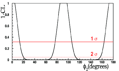
Figure 2: 1$-$C.L. vs. $\phi_{2}(\alpha)$ obtained from the isospin analysis of $B\to\rho\rho$ decays.

On the other hand, we find excesses in $B^{0}\to\rho^{0}\pi^{+}\pi^{-}$ and non-resonant $B^{0}\to\ 4\pi^{\pm}$ decays with 1.3$\sigma$ and 2.5$\sigma$ significance, respectively. We measure the branching fraction and 90% C.L. upper limit for $B^{0}\to\rho^{0}\pi^{+}\pi^{-}$ decay to be $(5.9^{+3.5}_{-3.4}\pm 2.7)\times 10^{-6}$ and $\mathcal{B}(B^{0}\to\rho^{0}\pi^{+}\pi^{-})<12.0\times 10^{-6}$. For the non-resonant $B^{0}\to\ 4\pi^{\pm}$ mode, we measure its branching fraction to be $(12.4^{+4.7+2.1}_{-4.6-1.9})\times 10^{-6}$ with a 90% C.L. upper limit of $\mathcal{B}(B^{0}\to 4\pi^{\pm})<19.3\times 10^{-6}$. For these limits we assume the final state particles are distributed uniformly in three- and four-body phase space. We find no significant signal for the decays $B^{0}\to\rho^{0}f_{0}$, $B^{0}\to\ f_{0}f_{0}$ and $B^{0}\to\ f_{0}\pi^{+}\pi^{-}$; the final results and upper limits are listed in Table 1.

We thank the KEKB group for excellent operation of the accelerator, the KEK cryogenics group for efficient solenoid operations, and the KEK computer group and the NII for valuable computing and SINET3 network support. We acknowledge support from MEXT and JSPS (Japan); ARC and DEST (Australia); NSFC (China); DST (India); MOEHRD, KOSEF and KRF (Korea); KBN (Poland); MES and RFAAE (Russia); ARRS (Slovenia); SNSF (Switzerland); NSC and MOE (Taiwan); and DOE (USA).

References

(1)N. Cabibbo, Phys. Rev. Lett. 10, 531 (1963); M. Kobayashi,
T. Maskawa, Prog. Theor. Phys. 49, 652 (1973).
(2)M. Gronau and D. London, Phys. Rev. Lett. 65, 3381 (1990).
(3)H. Ishino et al. (Belle Collaboration), Phys. Rev. Lett.
98, 211801 (2007); B. Aubert et al. (BaBar Collaboration),
Phys. Rev. Lett. 99, 021603 (2007).
(4)A. Somov et al. (Belle Collaboration), Phys. Rev. D
76, 011104 (2007); B. Aubert et al. (BaBar Collaboration),
Phys. Rev. D 76, 052007 (2007).
(5)A. Kusaka et al. (Belle Collaboration), Phys. Rev. Lett.
98 221602 (2007); B. Aubert et al. (BaBar Collaboration),
Phys. Rev. D 76, 012004 (2007).
(6)J. Zhang et al. (Belle Collaboration),
Phys. Rev. Lett. 91, 221801 (2003); B. Aubert et al.
(BaBar Collaboration), Phys. Rev. Lett. 97, 261801 (2006).
(7)H. Li, S. Mishima Phys. Rev. D 73, 114014 (2006).
(8)M. Beneke, J. Rohrer, D. Yang, arXiv:hep-ph/0612290.
(9)W. Zou, Z. Xiao, Phys. Rev. D 72, 094026 (2005),
arXiv:hep-ph/0507122.
(10)B. Aubert et al. (BaBar Collaboration), Phys. Rev. Lett.
98, 111801 (2007).
(11)B. Aubert et al. (BaBar Collaboration), Phys. Rev. D
78, 071104(R) (2008).
(12)K. Berkelman, Hadronic Decays, in B Decays ed. by S.
Stone, World Scientific, Singapore (1992).
(13)W. Adam et al. (DELPHI Collaboration), Z. Phys. C72,
207 (1996); P. Abreu et al. (DELPHI Collaboration), Phys. Lett.
B357, 255 (1995).
(14)S. Kurokawa and E. Kikutani, Nucl. Instrum. and Methods Phys.
Res. Sect. A 499, 1 (2003), and other papers included in this volume.
(15)A. Abashian et al. (Belle Collaboration), Nucl. Instrum.
and Methods Phys. Res. Sect. A 479, 117 (2002).
(16)Z. Natkaniec et al. (Belle SVD2 Group), Nucl. Instrum.
and Methods Phys. Res. Sect. A 560, 1 (2006).
(17)D. J. Lange, Nucl. Instrum. Methods Phys. Res., Sect. A
462, 152 (2001).
(18)E. Barberio and Z. Wa̧s, Comput. Phys. Commun. 79, 291
(1994); P. Golonka and Z. Wa̧s, arXiv:hep-ph/0506026.
(19)R. Brun et al., GEANT 3.21, CERN Report DD/EE/84-1,
1984.
(20)G. C. Fox and S. Wolfram, Phys. Rev. Lett. 41, 1581 (1978).
The modified moments used in this paper are described in S. H. Lee et al.
(Belle Collaboration), Phys. Rev. Lrtt. 91, 261801 (2003).
(21)H. Kakuno et al., Nucl. Instrum. and Meth. A 533, 516
(2004).
(22)H. Albrecht et al. (ARGUS Collaboration), Phys. Lett. B
241, 278 (1990).
(23)B. Aubert et al. (BaBar Collaboration), Phys. Rev. Lett.
97, 051802 (2006).
(24)E. Barberio et al. (Heavy Flavor Averaging Group),
arXiv:0704.3575 [hep-ex] and online update for winter 2008 at
http://www.slac.stanford.edu/xorg/hfag/rare/index.html
(25)A. Falk et al., Phys. Rev. D 69, 011502(R) (2004).