A method for characterization of coherent backgrounds in real time and its application in gravitational wave data analysis

Abstract

Many experiments, and in particular gravitational wave detectors, produce continuous streams of data whose frequency representations contain discrete, relatively narrowband coherent features at high amplitude. We discuss the application of digital Fourier transforms (DFTs) to characterization of these features, hereafter frequently referred to as lines. Application of DFTs to continuously produced time domain data are achieved through an algorithm [7], hereafter referred to as EFC, for efficient time-domain determination of the Fourier coefficients of a data set. We first define EFC and discuss parameters relating to the algorithm that determine its properties and action on the data. In gravitational wave interferometers, these lines are commonly due to parasitic sources of coherent background interference coupling into the instrument. Using GEO 600 data, we next demonstrate that time domain subtraction of lines can proceed without detrimental effects either on features at frequencies separated from that of the subtracted line, or on features at the frequency of the line but having different stationarity properties.

1 Introduction

The purpose of this paper is to describe and validate a method for characterizing and removing coherent backgrounds, hereafter referred to as lines, in continuously acquired data. There has been much work in this area, including several studies of techniques intended specifically for application to data from gravitational wave detectors. See for example references [1, 2, 3, 4, 5]. These existing methods make very limited use of Fourier coefficients, because the usual methods for obtaining these coefficients through the fast Fourier transform (FFT) algorithm [6] run into practical difficulties where it is required that the Fourier coefficients be equally accurate estimators of line parameters for all data samples, and that the estimate of line parameters be sufficiently fast to keep pace with the data sampling rate.

In this paper, we describe the application of an alternative to the fast Fourier transform, referred to throughout the paper as EFC, for obtaining the Fourier coefficients continuously updated at the data sampling rate. This algorithm was described in 1966 by Halberstein [7], and is the subject of U.S. and E.U. patents. See [8, 9], for example. The authors exploit this algorithm for the monitoring of coherent backgrounds in gravitational wave detector data. We demonstrate that EFC is significantly faster than real time running on contemporary computers, and equally accurate for all data samples. We continue by providing a proof of principle of EFC using data from a ground-based gravitational wave detector, and by studying the response of the algorithm to injected signals.

A key application of a robust real time capable line removal tool is the generation of triggers for networks of interferometric gravitational wave detectors in real time for the purposes of providing data for follow up of triggers with optical or radio observations. Applications of EFC in this area are more widespread than the removal of lines. A continuously maintained monitor of magnitude and phase of coherent signals in the data has many applications in gravitational wave interferometery, including calibration of the detectors, monitoring interferometer subsystems such as high Q suspensions, and studies of bicoherence between lines and features at other frequencies in the same data.

2 Line parameterization with Fourier transforms

By a line we mean an oscillating feature in the data whose amplitude $A_{i}$ at the time, $t_{i}$, of the $i^{\mathrm{th}}$ sample can be written

$$A_{n}=A_{0}\cos(2\pi ft_{n}+\phi),$$ (1)

where $A_{0}$, $f$, and $\phi$ are the underlying amplitude, frequency, and phase of the spectral feature, which are functions of time $t$. The algorithm we will describe requires that these parameters do not vary significantly on timescales less than some cutoff $\tau$. We will also confine the discussion to lines having $f(t)$ combined to a well defined domain for all $t$, and to data sampled regularly, meaning that the sampling time, $t_{s}=t_{n+1}-t_{n}$, is independent of $n$.

If the frequency $f$ is known precisely, it only remains to evaluate the amplitude $A$ and phase $\phi$ at each time $t_{n}$. A natural starting point would be the $k^{\mathrm{th}}$ coefficient of the digital Fourier transform [14] of $N$ successive data samples $x_{j}$ centered on the $n^{\mathrm{th}}$ data sample.

$$\mathcal{F}_{k}(x_{0},~{}x_{1},\cdots,x_{N-1})=\sum_{j=0}^{N-1}x_{j}e^{\frac{-2\pi ijk}{N}},$$ (2)

where $k\simeq Nt_{s}f$ and $Nt_{s}\leq\tau$. In the case where $f$ is not precisely known, or corresponds to non-integer $k$, the values of several Fourier coefficients would be needed. Fourier coefficients can be extracted from the DFT of the data, which is frequently calculated using a fast Fourier transform (FFT) algorithm [14, 15]. The number of floating point operations to calculate the DFT of $N$ successive data points is of order $N\log_{2}N$.

This method is beset with difficulties in the case where one requires a continuous, sample-by-sample estimator of $A$, $f$ and $\phi$. Because fast Fourier transform algorithms require a block of time series data, it is not obvious how to proceed from an estimate of $A_{n}$ and $\phi_{n}$ at the $n^{\mathrm{th}}$ data sample to an estimate of the $A_{n+1}$ and $\phi_{n+1}$. It is too computationally intensive to perform an FFT for each time sample - $N$ samples would require order of $N^{2}\log_{2}N$ operations. The alternative usually considered is performing a new FFT every $m$ samples, where $m<N$. The problem in this case is the occurrence of discontinuities in the estimator at each new transform.

3 The evolving Fourier coefficient (EFC) algorithm

In the case under discussion, only a restricted number of Fourier coefficients are of interest, suggesting an alternative approach. One starts by generating Fourier coefficients of $N$ data points using Equation 2. It is shown in A that the $k^{\mathrm{th}}$ Fourier coefficient, $\mathcal{F}_{k}(x_{1},~{}x_{2},\cdots,x_{N})$, of time samples $x_{1},~{}x_{2},\cdots,x_{N}$ is related to $\mathcal{F}_{k}(x_{0},~{}x_{1},\cdots,x_{N-1})$ by

$$\mathcal{F}_{k}(x_{1},~{}x_{2},\cdots,x_{N})=e^{\frac{+2\pi ik}{N}}\left(\mathcal{F}_{k}(x_{0},~{}x_{1},\cdots,x_{N-1})+(x_{N}-x_{0})\right).$$ (3)

Using this result, the computation of the Fourier coefficient of the overlapping time series is achieved without the need for an additional Fourier transform. The process can be repeated to obtain the time evolution of the Fourier coefficient for all subsequent time samples. Figure 1 illustrates the algorithm for the case where the sum is over four successive data samples.

We recall some properties of discrete Fourier transforms whose choice will be important in practical application of this technique to line monitoring and removal. First, the Fourier coefficient determines the line parameters over a data set of duration $\tau=Nt_{s}$. This timescale should be shorter than the typical timescale for variations in the line parameters $A$, $f$ and $\phi$, but longer than the typical timescale for features in the data that you would not wish to influence the line parameterization. The duration $\tau$ also determines the resolution bandwidth $B=1/\tau$, the bandwidth in frequency space sampled by a single Fourier coefficient. If the lines under study have a width or range of wander $\Delta f$, then the number of Fourier coefficients to be calculated is $\tau\Delta f=Nt_{s}\Delta f$ per new time sample.

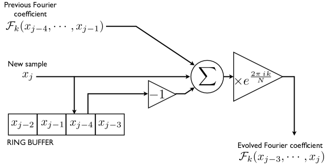
Figure 1: A block diagram illustration of the operation of the EFC algorithm for the simple case where each FFT is over four data samples. In the example iteration illustrated here, the sum of the new data sample and minus a data sample taken four sampling times previously are added to the previous Fourier coefficient, and the result of this sum is multiplied by $\exp(i\delta)$, where $\delta=2\pi k/N$ is the phase difference between successive time samples at the frequency of the Fourier component. The newest data sample then replaces the fifth most recent data sample in the ring buffer.

EFC requires an initial value for each Fourier coefficient of the data. We note, however, that if we use zeros for the values of $x_{0}$ subtracted in Equation 3 for the first $N$ timesamples, the output of the algorithm exactly equals the Fourier component after $N$ iterations. Hence there is no need for initial values of the Fourier components, since the iteration algorithm generates them. Equation 3 implies that the algorithm must evaluate the difference between the most recent data value $x_{N}$ and the data value $x_{0}$ acquired $N+1$ sampling times previously. After startup of the algorithm, the latter sample is unavailable until $N$ sampling times have elapsed, hence there is an unavoidable start-up period of $Nt_{s}$ to initialize the filter during which the algorithm output is not useful for line characterization. The response of the algorithm to transients is discussed in Section 4.6. A natural and fast way to implement access to the $N+1$ most recent data samples is to store $N$ previously acquired samples in a ring buffer, where at each iteration the oldest stored sample $x_{0}$ is read, applied in the algorithm, and then overwritten with the most recent sample $x_{N}$. A counter is then incremented, modulo $N$, so that the next element in the ring buffer, containing the input data value to be used as $x_{0}$ in the next iteration of Equation 3, is referenced.

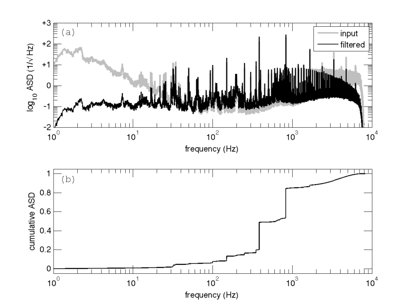
Figure 2: Amplitude spectral density (ASD) of noise from the GEO 600 michelson photodiode channel G1:LSC_MIC_VIS. The upper plot shows amplitude per $\surd$Hz as a function of frequency, where each bin has a bandwidth of 7.8 mHz. The dashed and solid curves are of data before and after the whitening prefilter discussed in Section 4.1. The lower plot is the cumulative ASD of the whitened data, obtained by adding in quadrature successive bins from the bold curve in the upper plot and normalizing to the maximum value. Lines contributing significantly to the time domain amplitude of the signal are shown as large, discrete steps in the cumulative ASD.

4 Tests on GEO 600 data

4.1 Characteristics of the test data

The immediate application for which the algorithm was conceived is the removal of coherent noise backgrounds from data produced by gravitational wave interferometers, such as the GEO [16], LIGO [11], VIRGO [12] and TAMA [13] instruments. For a general review of the science of direct gravitational wave detection the reader is referred to [10].

The tests of EFC described in this paper were carried out on data acquired from the GEO 600 gravitational wave interferometer through the LSC-Virgo scientific collabration. The GEO600 detector has been described in detail elsewhere [16]. For the purposes of testing this algorithm, an arbitrary 1000 seconds of data from the G1:LSC_MIC_VIS channel, sampled at 16384 Hz, and acquired when the instrument was in maintenance mode, was used. This signal represents a measurement of the DC light power reflected from the Michelson at the input port, commonly referred to as the common-mode visibility.

Figure 2 shows the amplitude spectral density (ASD) of the data before filtering. Plot (a) shows power spectral density over 7.8 mHz bins from 1 Hz to 8192 Hz, the Nyquist frequency of the data acquisition system. The dotted curve on this plot shows the ASD of the raw data. Broadband noise below 50 Hz and above 1 kHz dominates the cumulative amplitude spectral density. These components are suppressed using an IIR whitening filter [14] consisting of two zeros at 0 Hz, two real poles at 50 Hz and a single real pole at 1 kHz. The solid curve is an ASD of the data after this preprocessing step.

Plot (b) from figure 2 shows a cumulative ASD, obtained by squaring the ASD of the prefiltered data, integrating over frequency, taking the square root of the result, and dividing by the contents of the highest frequency bin. Line features in the data making the largest contributions to the overall signal amplitude appear as steps in the cumulative ASD. Table 1 column 1 shows the frequencies of some of these lines.

Table 1: Performance of the subtraction algorithm for the fifteen lines treated in the test. At each frequency (column 1), a number of bins (column 3) corresponding to a bandwidth (column 2) about the line centre were treated with the subtraction algorithm. After subtraction, the percentage shown in column 4 of the line amplitude before subtraction remained. Line amplitudes were determined using the frequency bin having the maximum ASD before subtraction.

Frequency (Hz)	Bandwidth (Hz)	Number of bins	Remnant (%)
150	1	8	7.1
250	1	8	8.5
350	1	8	8.8
384	2	16	1.3
550	1	8	14
614	5	40	1.3
650	1	8	16.3
709	5	40	1.2
803	2	16	9.4
828	5	40	0.44
1391	2	16	3.8
1654	5	40	0.79
3308	2	16	24

4.2 Line removal

The practical application of equation 1 to remove lines in the data is to estimate the amplitude and phase of oscillatory components of the preprocessed data at the frequencies of identified lines, to synthesize an oscillation having this amplitude and phase, and to subtract this oscillation from the data. The first step on receiving a new sample of data $x_{k}$ is to use equation 1 to generate an updated Fourier component $y_{k}$. The real part of this Fourier component is proportional to the wave of frequency $k/Nt_{s}$ contributing to the data. Note, however that the phase of $y_{k}$ represents the phase at the beginning of the timeseries, whereas for subtraction we require the phase half way through the timeseries . Therefore $y_{k}$ is modified by a phase factor representing the phase shift over $N/2-1$ samples, and then the real part of the result is taken. The correction signal is denoted $s_{k}$, and is given by

$$s_{k}=\frac{2}{N}\Re(y_{k}e^{i\pi k\left(1-\frac{2}{N}\right)}),$$ (4)

where $N$ and $y_{k}$ have the same meaning as in Section 3 and $\Re$ denotes the real part. One final important detail is the time lag between the data and the correction. $y_{k}$ is the Fourier component of input data $x_{k-N+1}\cdots x_{k}$, therefore it best represents the amplitude and phase of the corresponding frequency component at data sample $k-N/2$. Therefore the actual subtraction of the synthesized wave is performed on a timesample $N/2$ sample times lagging behind the $k^{\mathrm{th}}$ input sample. In this sense the line subtraction filter is acausal; it requires data both before and after the point of interest to determine the correction at that point. For post-processing removal of lines, for example as part of an off-line analysis chain, this is not a problem. The line subtracted data set $\{r_{k}\}$ is given by

$$r_{k-N/2}=x_{k-N/2}-s_{k}$$ (5)

for all $k$. Note that the above equation subtracts a synthesized wave representing only one Fourier component from the data set. The method can be applied to multiple components, and to lines spanning more than one bin in Fourier space. The bandwidth of adjacent frequency bins is the reciprocal of the time duration of the equivalent Fourier transform.

4.3 Computational overhead of the processing algorithm

A practical line removal algorithm must be able to process the data at a rate at least as high as the production rate for the data set. Fast data channels from existing gravitational wave detectors sample at $t_{s}=1/16384~{}\mathrm{s}$. The algorithm was implemented in the programming language C, and benchmarked on a MacBook Pro having a clock speed of 2.33 GHz and an Intel Core 2 Duo chipset, using the ANSI C time library and the computer’s on-board clock. The time per incoming data sample per Fourier component analyzed was 1/1700 of $t_{s}$, so the code can process 1700 Fourier components in parallel on a single CPU and match the incoming data rate. Because each Fourier component is treated separately, the algorithm could be run on a cluster in which case the number of frequencies treated is limited only by the number of cluster nodes. Tests on an intel based PC running linux yielded 1730 Fourier components in $t_{s}$.

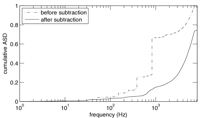
Figure 3: Cumulative amplitude spectral density (ASD) of noise from the GEO 600 michelson photodiode channel G1:LSC_MIC_VIS before and after subtraction of the lines listed in Table 1. Both curves are scaled to the maximum of the cumulative amplitude spectral density of the unsubtracted data. At the Nyquist frequency, the amplitude of the line subtracted data is 0.54 that of the unsubtracted data.

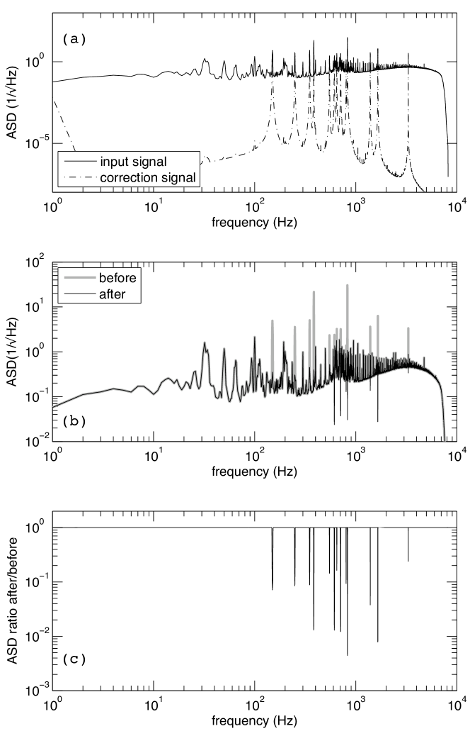
Figure 4: ASD of noise before line subtraction with the amplitude spectral density of the subtracted waveform overlaid - plot (a). ASD of the noise before (black) and after (grey) line subtraction - plot (b). Ratio of the ASD after to before line subtraction versus frequency - plot (c). The efficiency of line removal, defined as one minus the ratio of the ASD after to before at the line peak, is better than 76% for all the lines.

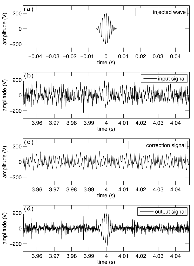
Figure 5: Time series 50 ms of data before (b), and after (d) the subtraction of the correction signal (c) generated using the MFT algorithm. So (b) is the sample-by-sample sum of (c) and (d). A sine-gaussian having the same sine wave frequency as the subtracted line (828 Hz), shown in plot (a), was added to the data in plot (b) to show that even bursts at line frequencies are unaffected by line subtraction as long as their duration is much less than the response time of the filter.

4.4 Performance on the test data

Performance on the test data is summarized in Figures 3, 4, and 5. Figure 3 shows the cumulative ASD before and after subtraction on the same scale. The r.m.s. amplitude of the prewhitened data is reduced to 0.54 of its unprocessed value after line removal. Figure 4 shows the ASD of the input data with the ASD of the correction superimposed; as expected the correction signal is dominated by sharp peaks at the frequencies of each of the corrected lines. Plot (b) of this figure shows the ASD of the data before and after line subtraction overlaid. Plot (c) shows the ratio of the bin-by-bin ASDs of the data after to before line removal; each line is removed to a maximum of 24% of its pre-treatment value, with the largest lines (having the highest SNR in the power spectrum) attenuated to 0.6% of their amplitude in the input data. The 4^th column of Table 1 shows the percentage of the pre-subtraction ASD remaining at the Fourier component dominating the line after subtraction. These numbers correspond to the depth of the dips at the line frequencies in Figure 3, plot (c).

4.5 The effect of a noise background

Noise in the subtracted signal enters through the noise background in the frequency bin being monitored. This noise background is considered here as broadband Johnson noise having a flat amplitude spectral density across the bin. As discussed in Section 3, the bandwidth of a single bin is given by $B=1/\tau$ where $\tau$ is the duration of the timeseries used to estimate each Fourier coefficient. If the amplitude of the signal is $A_{S}$ and the noise has an amplitude spectral density $\lambda_{N}~{}/\surd{\mathrm{Hz}}$, then the signal to noise ratio in power, $\mathrm{snr}$ is given by

$$\mathrm{snr}=\frac{A_{S}^{2}\tau}{\lambda_{N}^{2}}$$ (6)

If subtracting the line with a given $\tau$ leads to addition of noise, the only recourse is to increase $\tau$, and therefore decrease the bandwidth sampled per Fourier coefficient. In the case where the line covers several bins in frequency space, the number of Fourier coefficients subtracted will rise as you increase $\tau$, resulting in an increase in CPU usage proportional to the increase in $\tau$. In addition, larger $\tau$ increases the response time of the filter. As discussed in Section 4.6, this will make the subtraction insensitive to a greater range of time durations of bursts, which may be desirable from the point of view of signal searches. On the other hand, $\tau$ should not be so large that it exceeds the timescales typical of fluctuations in the amplitude or phase of a Fourier component of the line. The authors found that $\tau$ of the order of 8-32 seconds satisfied these requirements for the lines detailed in Table 1. Relating signal to noise ratio to efficiency of the line remover, lower signal to noise ratio leads to less efficiency in line removal. If the frequency of the line is stable and its parameters are slowly varying, one can still increase efficiency by increasing $\tau$. Otherwise the line subtraction is unavoidably inefficient. However, where the main aim of this tool is to suppress lines that make significant contributions to the cumulative ASD, and therefore to the time domain amplitude of the data stream, we observe that all lines corresponding to discernable steps in the cumulative ASD have been efficiently removed after subtraction.

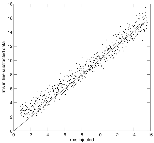
Figure 6: Amplitude of sine gaussian signals after they have been injected at random positions in a 256 second segment of data, and after the line remover has been run, versus the amplitude of the signal before injection. Both amplitudes are expresssed in units of the r.m.s. of the data before injections. There were 500 injections with amplitudes of between 0.78 and 15.23 times the r.m.s. noise level. As a guide to the eye, a straight line of slope one through the origin is also plotted.

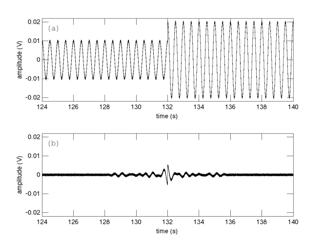
Figure 7: Response of the line removal algorithm to a large discrete step in amplitude of a line during subtraction. The line frequency is 2 Hz. Plot (a) shows the wave fed to the line removal algorithm, consisting of the oscillation having an RMS amplitude of 7 mV before 132 s and 14 mV after this time, plus pseudorandom gaussian distributed noise with an RMS of 0.2 mV throughout. Plot (b) shows the data after line subtraction in the 16 seconds surrounding the discontinuity. The effects of the discontinuity are confined to the 8 second interval around the discontinuity. Note that the amplitude of the line relative to the noise is far greater than in the engineering data so that the effect of the discontinuity is clear above the noise background.

4.6 Response of the algorithm to injected signals

Figure 5 shows the response of the subtraction algorithm to a representative sample of the test data, but in addition a single short time duration sine Gaussian burst has been added to the data. The ratio of the peak signal amplitude to the R.M.S. amplitude of the data was 3.125. Plot (a) of this figure shows the added burst. This particular burst has been selected as a worst-case scenario, since the frequency of the oscillations inside the envelope is 828 Hz, exactly equal to a dominant line frequency in the data. Plots (b), (c) and (d) show, respectively, the input data after the test signal has been added, the correction signal generated from the data for the same time segment, and the result of subtraction of this correction signal. The signal survives in the line subtracted data, but the persistent fluctuations from background noise are removed. This separation is possible due to the response time of the filter. The Fourier components are measured over a time duration of $\tau=8$ seconds, so that any fluctuations in the line parameters on a timescale much shorter than $\tau$ are not significantly corrected by the filter. This is a critical feature of this algorithm for line tracking - the response time of the line tracker can be set based on knowledge of the properties of the noise (the stability of the line noise background) and the signal, the expected time duration of any transient signals that one may wish to avoid suppressing.

Signal injections were next made at 500 random times in a 256 second data segment, where the amplitude of the injection was varied between 0.78 and 15.23 times the r.m.s. noise level. The mean separation between injections was approximately 0.5 seconds, an average of 16 injections per Fourier transform duration. After signal injection, the line subtraction algorithm was applied, then the maximum height of the data in the domain of each injected signal was measured. This maximum height was plotted against the height of the original injected signal in Figure 6. At small injection amplitudes, the maximum height after injection reflects the noise background, since the probability of random noise fluctuations under the signal leading to at least one bin that exceeds the original injection amplitude increases as the signal to noise ratio decreases. At large injection amplitude, the ratio of amplitudes after to before injection fluctuates about one. This behaviour is consistent with the maximum height bin in the line subtracted data being that having the maximum amplitude in the injected signal, but to this maximum height is added a noise term that either increases or decreases the overall amplitude by an amount having the probability distribution of the noise background.

The response of the line removal algorithm to a discontinuous step in the parameters of a line was also investigated. Figure 7 shows the results of this investigation. The input data, consisting of a 2 Hz sine wave having an RMS amplitude of 7 mV, had its rms amplitude stepped discontinously to 14 mV at a time of 132 seconds on this scale. Plot (b) shows the output of the filter. Note that the input waveform has been delayed by 4 seconds to account for the time delay between the input signal and the correction signal discussed in Section 4.2, so that the time axis on both plots represents the time at which the signal correction was applied to the data, 4 seconds after the input data that generated the correction. The acausality of the filter is clearly visible in plot (b). The injection time of the discontinuity was at 128 seconds, corresponding to a correction time of 132 seconds, but before this time and after 128 seconds the effects of the discontinuity are already apparent in plot (b). Note, however, that the effects of the discontinuity are completely confined to the 8 seconds surrounding the correction time, because the Fourier coefficients used to evaluate the line parameters are evaluated over $\tau=8$ s.

5 Summary

The line subtraction method discussed in this paper successfully removes at least 76% of the peak amplitude of all frequency-stable lines to which it has been applied in test data. For lines for which a high signal to noise ratio can be achieved, over 99% of the line amplitude can be removed. Tests so far have focussed on data acquired at a sampling rate of 16,384 Hz, because this is the sampling frequency of fast channels in the GEO and LIGO data acquisition systems. At this sampling frequency, the algorithm can subtract 1700 separate frequencies in parallel on a single CPU, and still keep up with the incoming data rate. If the rate were 16.384 MHz, at least 1 frequency subtraction would still be possible in real time. Because the algorithm operates on each frequency component separately, it is amenable to parallelization, in which case as long as at least one frequency can be processed in real time on each CPU, the number of frequencies subtracted depends only on the number of CPUs.

Applications of line-removal in gravitational wave data analysis are wide-ranging. This technique could be used as a pre-processing step for existing burst search algorithms, and may also be useful in searches for other types of signals. Furthermore, it presents the prospect of obtaining a very white spectrum of time domain strain data in the gravitational wave channel. If applied successfully, the spectral density would be frequency independent. This would allow for more robust time domain searches for unmodelled bursts, where the search sensitivity is strongly dependent only on the amplitude of a burst signal and only weakly dependent on its shape. The method is also applicable to other problems where it is desirable to monitor the amplitude and phase of a wave of known frequency, sample by sample, online. Applications in this category will be discussed in a future publication.

6 Acknowledgements

Support for this work was through a Marie Curie international reintegration grant no. FP6-006651. The authors would also like to thank the operators of the GEO 600 instrument for furnishing the data used to test this algorithm. This paper was assigned LIGO document number P080013.

Appendix A Proof of the EFC evolution formula for Fourier coefficients

This proof starts with equation 2 for the $k^{\mathrm{th}}$ Fourier coefficient, where we separate the $j=0$ term from the sum and write it at the end.

$$\mathcal{F}_{k}(x_{0},~{}x_{1},\cdots,x_{N-1})=\sum_{j=1}^{N-1}x_{j}e^{\frac{-2\pi ijk}{N}}+x_{0}.$$ (7)

Next write down an expression below for the $k^{\mathrm{th}}$ Fourier coefficient of the data forward timeshifted by one sample, where the new sample is $x_{N}$. Rearrange this expression by separating the term in $x_{N}$ and factor out a common phase.

$$\mathcal{F}_{k}(x_{1},~{}x_{2},\cdots,x_{N}) = \sum_{j=1}^{N}x_{j}e^{\frac{-2\pi i(j-1)k}{N}}$$

$$= \sum_{j=1}^{N-1}x_{j}e^{\frac{-2\pi i(j-1)k}{N}}+x_{N}e^{\frac{-2\pi i(N-1)k}{N}}.$$

$$= e^{\frac{+2\pi ik}{N}}\left(\sum_{j=1}^{N-1}x_{j}e^{\frac{-2\pi ijk}{N}}+x_{N}e^{\frac{-2\pi iNk}{N}}\right)$$

$$= e^{\frac{+2\pi ik}{N}}\left(\sum_{j=1}^{N-1}x_{j}e^{\frac{-2\pi ijk}{N}}+x_{N}\right).$$

The expression in parentheses can be related to $\mathcal{F}_{k}(x_{0},~{}x_{1},\cdots,x_{N-1})$ by using equation 7.

$$\mathcal{F}_{k}(x_{1},~{}x_{2},\cdots,x_{N})=e^{\frac{+2\pi ik}{N}}\left(\mathcal{F}_{k}(x_{0},~{}x_{1},\cdots,x_{N-1})+(x_{N}-x_{0})\right).$$ (9)

This is the desired result.

References

References

- [1] S. D. Mohanty, Class. Quantum Grav. 19 1513-1519 (2002)
- [2] L. S. Finn and S. Mukherjee, Phys. Rev. D 63 062004 (2001)
- [3] A. M. Sintes and B. Schutz, Phys. Rev. D 58 122003 (1998)
- [4] B. Allen, W. Hua and A. C. Ottewill, gr-qc/9909083
- [5] E. Chassande-Motin and S. V. Dhurandhar, Phys. Rev. D 63 042004 (2001)
- [6] J. W. Cooley and J. W. Tukey, Mathematics of Computation 19 no. 90, 297-301 (1965)
- [7] J. H. Halberstein, Proc. IEEE 54 903 (1966)
- [8] J. W. Schmitt and D. L, Starkley, U.S. Patent 3,778,606 (1973)
- [9] K. Takaoka and K. Yokosuka-Shi, E.U. Patent EP 1 176 516 A2 (2001)
-
[10]
J. Hough and S. Rowan, Living Rev. Relativity
3 lrr-2000-3 (2000)
http://relativity.livingreviews.org/Articles/lrr-2000-3/ - [11] A. Abramovici et al. Science 256 no. 5055, 325-333
- [12] C. Bradaschia et al. Nucl. Instrum. Meth. A 289 518-525 (1990)
- [13] M. Ando et al. Phys. Rev. Lett. 86 3950 (2001)
- [14] A.V. Oppenheim, R.W. Schafer, “Digital Signal Processing”, ISBN 0-13-214635-5, Prentice Hall, 1975.
- [15] W.H. Press, S.A. Teukolsky, W.T. Vetterling, B.P. Flannery, “Numerical Recipes in C”, ISBN 0-521-43108-5, Cambridge University Press, 1992.
- [16] B. Willke et al., Class. Quant. Grav. 19 (2002) 1377.