Localized states and interaction induced delocalization in Bose gases with quenched disorder

Abstract

Very diluted Bose gas placed into a disordered environment falls into a fragmented localized state. At some critical density the repulsion between particles overcomes the disorder. The gas transits into a coherent superfluid state. In this article the geometrical and energetic characteristics of the localized state at zero temperature and the critical density at which the quantum phase transition from the localized to the superfluid state proceeds are found.

1 Introduction

The interplay between interaction and disorder is an important paradigm of condensed matter physics. In 1958 Anderson[1] showed that in disordered solids a non-interacting electron may become localized due to the quantum interference. A phenomenological theory of localization[2, 3] concluded that non-interacting electrons in one and two dimensions are always localized. In three dimensions the localized and extended states are separated by the mobility edge. States with energy significantly below this edge in 3 dimensions are strongly localized. They appear in rare fluctuations of the quenched random potential[4, 5, 6]. These instanton-type states broaden and eventually overlap with growing energy. A system of non-interacting fermions in the random potential transits from the insulator to metal state when its Fermi energy exceeds the mobility edge. Thus, the Pauli principle delocalizes fermions in 3 dimensions, but leave them localized in lower dimensions. The common belief is that the repulsive interaction suppresses the localization. So far this problem was studied only in the limit of a weak disorder[7, 8]. Therefore, the interaction induced delocalization transition remains beyond the frameworks of the theory. The metal-insulator transition in 2 dimensions was observed in experiments[9] suggesting the decisive role of interaction. The physical picture changes drastically for bosons. The non-interacting bosons condense at a single-particle state with the lowest energy. In a homogeneous system it leads to a coherent quantum state known as the Bose-Einstein condensate (BEC). Examples are superfluid phases of He[10], superconductors [11], BEC of ultra-cold alkali atoms[12, 13] and of excitons in semiconductors[14]. BEC still persists when a small amount of disorder is added to the system. BEC in a random environment was observed in the superfluid phase of ⁴He in Vycor glass or aerogels[15] , in ³He in aerogels[16] and in ultra-cold alkali atoms in disordered traps [17, 19, 18, 20, 21, 22, 23]. But in a random environment and in the absence of interaction, all Bose-particles fall into the lowest localized single-particle state. Such a ground state is non-ergodic since its energy and spatial extension depend on a specific realization of the disorder. An arbitrary small repulsive interaction redistributes the bosons over multiple potential wells and restores ergodicity. Hence, contrary to the fermionic case, the perturbation theory with respect to the interaction strength is invalid. At low temperature, the Bose systems display superfluidity provided the density $n$ of bosons exceeds a critical value $n_{c}$. At either weak disorder or strong interaction, i.e. at $n\gg n_{c}$, the disorder corrections to the superfluid density $n_{s}$ (and the condensate density $n_{0}$) are small[24, 25, 26] . These correction blow up with the interaction decreasing, signaling the breakdown of the theory.

We present an alternative approach to the problem of the interaction-induced delocalization starting from deeply localized state of the Bose-gas in a random potential. We present a simple and visual picture of the deeply localized state, which decays into remote weakly coupled fragments. We give a geometrical description of fragments and their distribution in space. At a critical density $n_{c}$, which we express in terms of the disorder characteristic and interaction strength, the increasing tunneling of particles between fragments leads to transition from the random singlet state to the coherent superfluid.

2 Single-particle levels in an uncorrelated random potential

The random environment produces a random potential $U(\textbf{x})$ for the bosons. We assume that $U(\textbf{x})$ is Gaussian distributed with zero average and short range correlations

$$\left\langle U\left(\mathbf{x}\right)U\left(\mathbf{x}^{\prime}\right)\right\rangle=\kappa^{2}\delta(\textbf{x}-\textbf{x}^{\prime})$$ (1)

We will consider briefly the long range correlated case at the end of this article. In the absence of interaction the single-particle wave functions obey the the Schrödinger equation

$$\frac{\hbar^{2}}{2m}\nabla^{2}\psi+\left(E-U\left(\mathbf{x}\right)\right)\psi=0.$$ (2)

Its energy levels $E\left[U\left(\mathbf{x}\right)\right]$ are functionals of the potential $U\left(\mathbf{x}\right)$. The only characteristic of the random potential $\kappa$ together with the Planck’s constant $\hbar$ and the mass $m$ establishes the scales of length and energy:

$$\mathcal{L}=\frac{\hbar^{4}}{m^{2}\kappa^{2}},\,\,\,\,\,\,\,\,\,\mathcal{E}=\frac{\hbar^{2}}{m\mathcal{L}^{2}},$$ (3)

which we call the Larkin length and Larkin energy, respectively [27]. The density of states $\nu(E)$ belonging to (2) in the limit $E<0,|E|\gg{\cal E}$ was calculated in [4, 5, 6] (for a complete summary see [28]). For 3d system with the volume $\Omega$ it reads:

$$\nu(E)=\frac{1}{\Omega}\langle\delta\left(E-E\left[U\left(\mathbf{x}\right)\right]\right)\rangle\sim{\cal N}(E)e^{-(|E|/{\cal E})^{1/2}},$$ (4)

where we absorbed a numerical constant in the exponent of $\nu(E)$ in the definition of ${\cal E}$. As we show below the precise form of the prefactor ${\cal N}(E)$ is not relevant for our consideration. In a large 3d volume the states with energy $E\gg\mathcal{E}$ are delocalized, whereas the states with negative energy sufficiently large by modulus $E<0$ and $\left|E\right|\gg\mathcal{E}$ are strongly localized. The threshold of localization is a positive energy of the order of $\mathcal{E}$ [29]. In the interval between $\mathcal{E}$ and $-\mathcal{E}$ the transition from the extended to strongly localized states proceeds. The latter are supported by rare fluctuations of the random potential, which form a potential well sufficiently deep to have the negative energy $E$ as its only bound state. Let us introduce the spatial density $n_{w}(E)$ with the energy less than $E$. It is related to the DOS by equation $n_{w}(E)=\int_{-\infty}^{E}\nu(E)dE.$ For deep levels it can be also considered as the spatial density of states $n_{w}(R)$ with the radius less than $R$, where $R=\hbar/\sqrt{2m|E|}$. For such states $n_{w}(R)$ is proportional to a small exponent $\exp(-\sqrt{{\mid E\mid}/{\cal{E}})}=\exp(-{\cal{L}}/{R})$. From the dimensionality consideration it follows:

$$n_{w}(E)=R^{-3}f\left(\frac{\cal{L}}{R}\right)\exp\left(-\frac{\cal{L}}{R}\right).$$ (5)

The function $f(x)$ can be found from Ref.[30] to be proportional to $f(x)\sim x^{\alpha}$ with $\alpha=1$. It will be inessential for further calculation. The average distance $d(R)$ between the wells of the radius less than $R$ reads: $d(R)=n^{-1/3}_{w}=Rf^{-1/3}\exp\left(\frac{\cal{L}}{3R}\right)$. Thus, the distances between the wells are significantly larger than their sizes. The tunneling factor $t\left(R\right)$ between two typical wells with the radius $R$ of the same order of magnitude is given by a semiclassical expression $t\left(R\right)=\exp\left(-\frac{1}{\hbar}\int\left|p\right|\ dl\right)$, where the path of integration connects the two wells. By the order of magnitude $p\sim\hbar/R$ and the length of the integration path is $\sim d\left(R\right)$. Thus, $\frac{1}{\hbar}\int\left|p\right|\ dl\approx d/R\approx f^{-1/3}\exp{\left(\frac{\cal{L}}{3R}\right)}$ and

$$t\left(R\right)=\exp\left[-f^{-1/3}\exp\left(\frac{\cal{L}}{3R}\right)\right].$$ (6)

At $R\sim\mathcal{L}/3$ or $E\sim-9\mathcal{E}$, the distances between the optimal potential wells become of the same order of magnitude as their size $R$. Simultaneously the tunneling amplitude between the wells becomes of the order of 1. The potential wells percolate and tunneling is not small, but the states still are not propagating due to the Anderson localization [1].

3 Bose gas in a large box with an uncorrelated random potential

In the ground state of an ideal Bose gas in a large box with the Gaussian random potential all particles are located at the deepest fluctuation level. In the box of cubic shape with the side $L$ the deepest level which occurs with probability of the order of 1 has the radius $R$ determined by equation: $L^{3}n_{w}\left(R\right)=1$, i.e. $R\sim\frac{\mathcal{L}}{3\ln\left(L/\mathcal{L}\right)}$. The prefactor $f$ introduces a negligible correction to the denominator of the order of $\ln\left(\ln\frac{L}{\mathcal{L}}\right)$. The corresponding energy is $E\sim-9\mathcal{E}\left(\ln\frac{L}{\mathcal{L}}\right)^{2}$. As we already mentioned such a state is non-ergodic since the location and the depth of the deepest level strongly depends on a specific realization of the disordered potential. Therefore, the average energy per particle and other properties averaged over the ensemble has nothing in common with the properties of a specific sample. Even an infinitely small repulsion makes the system ergodic in the thermodynamic limit, i.e. when first the size of the system grows to infinity and then the interaction goes to zero. In a sufficiently large volume any physical value per particle coincides with its average over the ensemble. The reason of such a sharp change is that, at any small but finite interaction, the energy of particles repulsion overcomes their attraction to the potential well when the number of particles increases. They will be redistributed over multiple wells. Since the distribution of wells in different parts of sufficiently large volume passes all possible random configurations with proper ensemble probabilities, the ergodicity is established. Below we find how the interacting particles eventually fill localized states. In a real experiment the Bose gas may be quenched in a metastable state depending on the cooling rate and other non-thermodynamic factors. This is what M.P.A. Fisher et al. [31] call the Bose glass. Such a state is also possible in the case of weakly repulsive Bose gas. However, as it will be demonstrated later, in the case of cooled alkali atoms the tunneling amplitude still remains large enough to ensure the relaxation to the equilibrium state in 10${}^{-3}\div$10${}^{-2}s$. Our further estimates relate to the real ground state. As in the Bogolyubov’s theory [32] we assume that the gas criterion $na^{3}\ll 1$ is satisfied. Here $n=N/\Omega$ is the average particle density; $N$ is their total number and $a$ is the scattering length. Implicitly our considerations takes in account the change of the optimal potential well due to the interaction.

Let the Bose gas with the average density of particles $n$ fill all potential wells with the radii less than $R$ in the ground state. The average number of particles per well is ${N_{w}}\left(R\right)={n}/{n_{w}\left(R\right)}$. The local density inside the well of the linear size $R$ is $n_{p}(R)=\frac{3{N_{w}}\left(R\right)}{4\pi R^{3}}$. The gain of energy per particle due to random potential is $E\left(R\right)=-\frac{\hbar^{2}}{2mR^{2}}$; the repulsion energy due to interaction is equal to $gn_{p}\left(R\right)=\frac{3\hbar^{2}{N_{w}}\left(R\right)a}{mR^{3}}$, where we used the well-known relation for an effective potential field induced by a gas of scatterers [33]. Minimizing the total energy per particle $E_{tot}\left(R\right)=-\frac{\hbar^{2}}{2mR^{2}}+\frac{3\hbar^{2}{N_{w}}\left(R\right)a}{mR^{3}}$ over $R$ we find the value of $R$ corresponding to the minimum of energy at fixed $n$ with the logarithmic precision:

$$R\left(n\right)=\frac{\mathcal{L}}{\ln({n_{c}}/{n})}\,\,\,\,.$$ (7)

$\textrm{where}\,\,\,\,n_{c}=\left(3\mathcal{L}^{2}a\right)^{-1}$ denotes the critical density. The factor $f$ in equation (5) leads to corrections of the type $\ln\left(\ln({n_{c}}/{n})\right)$ which can be neglected. Further we put $f=1$. The distances between the filled wells according to the corresponding expression $d(R)$ for single-particle states reads $d\left(n\right)={\mathcal{L}}({\ln({n_{c}}/{n})})^{-1}\left({n_{c}/}{n}\right)^{1/3}$. They strongly exceed the average size of the potential well (7) at $n\ll n_{c}$. At the same condition the chemical potential of atoms can be estimated as $\mu\left(n\right)=-\frac{\hbar^{2}}{2mR^{2}\left(n\right)}=-\frac{\mathcal{E}}{2}\left(\ln\frac{n_{c}}{n}\right)^{2}$. The tunneling amplitude $t\left(n\right)$ between two wells separated by a typical distance $d\left(n\right)$ can be found by employing the single particle result (6):

$$t\left(n\right)=\exp\left[-\left({n_{c}}/{n}\right)^{1/3}\right].$$ (8)

Thus, the Bose gas at $n\ll n_{c}$ is fragmented into multiple clusters of small size $R\left(n\right)$ separated by much larger distances $d\left(n\right)$ and containing about $\mathcal{L}/\left[3a\left(\ln\frac{n_{c}}{n}\right)^{3}\right]$ particles each. The amplitude of tunneling between the wells depends on the scattering length in a non-analytic way and is exponentially small for weak interaction. Therefore, the number of particles in each cluster is well defined. As a consequence, the phase is completely uncertain. Such a state is a singlet with non-uniformly distributed particles, a random singlet: the ground state is non-degenerate. The compressibility $\frac{\partial n}{\partial\mu}=\frac{n}{\cal E}\ln\frac{n_{c}}{n}$ is finite as expected for the Bose glass phase [31].

4 Bosons in atomic traps

Our results can be easily extended to bosons in harmonic traps characterized by a potential

$$V_{trap}=\frac{m\omega^{2}R^{2}}{2}=\frac{\hbar^{2}}{2m}\frac{R^{2}}{\ell^{4}}$$ (9)

where we introduced the oscillator length $\ell=\sqrt{\hbar/(m\omega)}$. This section partly overlaps sligthly with our previous work [34]. The energy of the bosons includes now four terms: the kinetic energy, the confining potential energy of the trap, the repulsion from other particles and the energy of the random potential. Two of them, the interaction with the trap and the random potential tend to confine and localize the particle. Going through essentially the same steps as before, we can distinguish four different regimes (Figure 1).

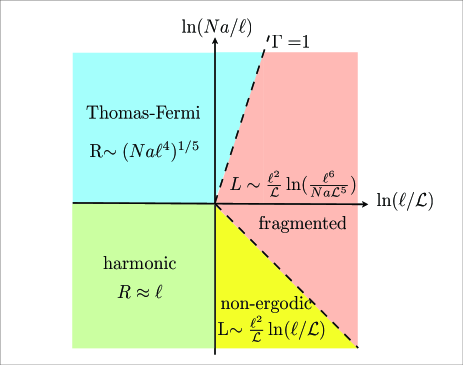
Figure 1: Regime diagram of atoms in traps: uncorrelated disorder. $R$ denotes the size of the single existing atomic cloud. $L$ is the size of the cloud of fragments.

1. Weak disorder and weak interaction: $3Na\ll\ell\ll\mathcal{L}$ . In this case the interaction can be neglected. Minimizing the remaining terms, the kinetic energy and energy of the trap, we find $R=\ell$. Physically it means that all particles are condensed in the oscillator ground state.

2. Weak disorder and strong interaction: $\ell\ll\mathcal{L},\,\,\ell\ll 3Na$ . Neglecting the kinetic energy and minimizing remaining energy of traps plus the repulsion energy, one finds the result known as Thomas-Fermi approximation[13]: $R=\left(\frac{9}{2}Na\ell^{4}\right)^{1/5}$.

3. Strong disorder and weak interaction : $3Na\ll\mathcal{L}\ll\ell$ . In this range of variables the non-ergodic phase is realized. Since interaction is negligible, the particles find a random potential well with the deepest level and fall into it. Let such a well can be found at a distance $\sim L$ from the trap center. Its depth typically is about $9\mathcal{E}\ln^{2}\left(L/\mathcal{L}\right)$. This gain of energy must be not less than the loss of the trap energy $m\omega^{2}L^{2}/2$. A typical value of $L$ appears when both this energies have the same order of magnitude. Thus, $L\approx 6\sqrt{2}\left(\ell^{2}/\mathcal{L}\right)\ln\left(\ell/\mathcal{L}\right)$. A typical size of the well is $R\approx\mathcal{L}/\left(6\ln\left(\ell/\mathcal{L}\right)\right)$.

4. Strong disorder and moderate interaction: $\mathcal{L}\ll 3Na\ll\ell$. In this case the ergodicity is restored. Our experience with the gas in a box prompts that the gas cloud is split into fragments each occupying a random potential well from very small size till same size $R$ depending on $N$. The typical disorder energy per particle is $\mu=-\mathcal{E}\left(\ln\frac{n_{c}}{n}\right)^{2}$. It becomes equal to the trap energy at the distance $L\sim\left(\ell^{2}/\mathcal{L}\right){\ln\Gamma}$ where $\Gamma$ is a new dimensionless parameter

$$\Gamma=\frac{\ell^{6}}{3Na\mathcal{L}^{5}}\sim\frac{n_{c}}{n}.$$ (10)

Therefore, the average density is $n\sim N\mathcal{L}^{3}/\ell^{6}$. The state of the Bose gas is fragmented and strongly localized when $\Gamma$ is large; the transition to delocalized superfluid state proceeds when this ratio becomes $\sim$1. The phase diagram is shown in Fig. 1. Note the counter-intuitive dependence of the size on the number of particles: the cloud slightly contracts with increasing number of particles. It happens because the number of particles in each fragment increases more rapidly with the average density than the number of fragments.

5 Correlated disorder

So far we considered uncorrelated disorder (1). Our results can be extended to random potentials with a finite correlation length $b$ and strength $U_{0}=\sqrt{\langle U^{2}\left(\bf{x}\right)\rangle}$. We quote here the results without derivation, which can be found in Ref. [36]. As long as $b\ll{\cal L}=\frac{3\hbar^{4}}{4\pi m^{2}U_{0}^{2}b^{3}}$ the results of the previous considerations remain correct. In the opposite case the optimal potential wells have the width $b$ and, contrary to the short range correlated case, they contain many bound states (of the order of $(b/{\cal L})^{3/4}\gg 1$). It is convenient to introduce a new length scale $B=b\left({\cal L}/{b}\right)^{1/4}=\left({3}/{4\pi}\right)^{1/4}\left({\hbar^{2}}/{mU_{0}}\right)^{1/2}$. In the following we restrict our consideration to the case $b\gg{\cal L}$, i.e. $b\gg B$. The density of states in this case is $\nu(E)\sim\exp[{-(E/U_{0})^{2}}]$ [28]. The critical density is $n_{c}\sim 1/(aB^{2})$ (this result has been found before in [35]) and the typical size of a fragment is $R\approx b(\ln(n_{c}/n))^{-1/2}$. The distance between fragments is $d(n)\approx b(n_{c}/n)^{1/3}$ and the tunneling coefficient is $t(n)\approx\exp[-(b/B)(n_{c}/n)^{1/3}]$.

In the case of a harmonic trap we again find four different regimes (Fig. 2). The relevant parameter is $\Gamma=\ell^{6}/(NaB^{5})\approx n_{c}/n$. For $\Gamma\approx 1$ the transition to the superfluid phase proceeds.

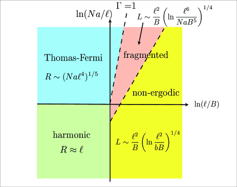
Figure 2: Regime diagram of atoms in traps: correlated disorder. $R$ denotes the size of the single atomic cloud, $L$ denotes the size of the fragmented state.

All results can be extended to lower dimensions [36].

6 Conclusions

Four parameters can be controllably and independently varied in the experiment. They are: number of particles $N$; the frequency $\omega$ or equivalently the strength of the trap; the scattering length $a$ (it can be varied by approaching one of the Feshbach resonances); the strength of disorder $U_{0}$. Using this freedom it is feasible to pass all regimes described above. A simple estimate shows that, at $b\sim 1\mu m$, the transition from uncorrelated to strongly correlated regime proceeds at frequency of disorder potential $\omega_{d}=\sqrt{2U_{0}/mb^{2}}\sim 1kHz$ which is accessible.

Simplest experiments are the measurements of the cloud size $L$ as a function of different variable parameters in the regime of multiple localized fragments. Theory predicts that in the regime of uncorrelated disorder the size of the cloud is proportional to $U^{2}_{0}/\omega$ . It also predicts very weak dependence of the size on the number of particles $\sim{\ln N}$. In the case of strongly correlated disorder the size of the cloud is proportional to $\omega U_{0}^{1/2}$; the dependence on $N$ also is weaker than in the uncorrelated regime: $L\propto\left(\ln N\right)^{1/4}$.

It would be important to observe the transition from non-ergodic state with one or few fragments to the ergodic state with many fragments and check that it happens at $N=\mathcal{L}/3a$ for uncorrelated disorder and at $N=\left({b^{3}}/{3aB^{2}}\right)$ for strongly correlated disorder.

Another feasible experiment is the time-of-flight spectroscopy after switching off both the trap and the random potential. In this experiment the distribution of particles over momenta (velocities) is measured. Its width $\Delta p$ is associated with the average size of the fragment $R$ by the uncertainty relation $\Delta p=\hbar/R$. It gives the opportunity to check the equation $R=\mathcal{L}/\ln\Gamma$ for the uncorrelated disorder or $R=\mathcal{L}/\ln\Gamma$ for correlated disorder. Installing a counter close to the trap, at a distance comparable to the size of the trap, would allow to register the oscillations of the particle flux due to discrete character of the fragmented state. This is an opportunity to find the distances between fragments and compare theory with experiment.

The transition between localized and delocalized coherent state in the random potential was found in several experiments (see Introduction). We propose to make more detailed measurement of the transition manifold and check our predictions.

An important question is whether the relaxation to the ground state can be reached during a reasonable time interval compatible with the time of experiment. We analyze this question for the uncorrelated or weakly correlated disorder. In this case the relaxation time due to tunneling can be estimated as $\tau=2\pi\omega_{n}^{-1}t^{-1}$, where $\omega_{n}\sim\frac{\mathcal{E}}{\hbar}\left(\ln\Gamma\right)^{2}$ is the characteristic frequency of the optimal potential well and $t\sim\exp\left[-\Gamma^{1/3}\right]$ is the tunneling coefficient (see eq. (8)). For numerical estimates we accept $\Gamma\sim 125$, $\ell\sim 10\mu m$, $b\sim\mathcal{L}\sim 1\mu m$, $a\sim 0.01\mu m$, $N\simeq 27,000$. Then $t^{-1}=148$ and $\tau\sim 0.06s$. The Larkin length can be increased by decreasing the amplitude of the random potential. Simultaneously, at fixed values $N$, $\ell$ and $a,$ the value $\Gamma$ decreases as $\mathcal{L}^{-5}$. This example shows that the equilibrium is accessible, though it is difficult to reach large ratio $\mathcal{L}/b$.

The closest to ours was the approach developed in the work Lugan et al. [20]. Apart from the fact that these authors considered only the 1-dimensional case, the main difference between our and their problems is that they considered the random potential with the exact lower boundary $U_{\rm b}$ and with on-site distribution function $W[U]\propto\exp[-c(U-U_{\rm b})]$ instead of a Gaussian distribution. Such a distribution allows deeply localized states only at energies $E$ close to the exact lower boundary $U_{\rm b}$. The corresponding fluctuations have the width R the broader the closer is $E$ to $U_{\rm b}$. It is clear that these levels are very different from those discussed above. If the random potential has the exact lower boundary, our theory is valid only if this boundary is separated from the most probable value of the potential by an energy interval strongly exceeding the energy dispersion. Then the localized states of our theory appear at intermediate energies between dispersion and $U_{\rm b}$.

- [1] \NameAnderson P. W. \REVIEWPhys. Rev.10919581492.
- [2] \NameAbrahams E., Anderson P. W., Licciardello D. C. Ramakrishnan T. V. \REVIEWPhys. Rev. Lett.421978673.
- [3] \NameLee A. Ramakrishnan T. V. \REVIEWRev. Mod. Phys.571985287.
- [4] \NameLifshitz I. M. \REVIEWSov. Phys. JETP261968462.
- [5] \NameZittartz J. Langer J. \REVIEWPhys. Rev.1481966741.
- [6] \NameHalperin B. I. Lax M. \REVIEWPhys. Rev.1531966802.
- [7] \NameAltshuler B. L. Aronov A. G. \REVIEWSov. Phys. JETP501979968.
- [8] \NameFinkelstein A. M. \REVIEWSov. Phys. JETP57198397.
- [9] \NameAbrahams E., Kravchenko S. V. Sarachik M. P. \REVIEWRev. Mod. Phys.732001251.
- [10] \NameLeggett A. J. \REVIEWRev. Mod. Phys.732001307.
- [11] \NameSchrieffer J. R. Tinkham M. \REVIEWRev. Mod. Phys.711999313.
- [12] \NameKetterle W. \REVIEWRev. Mod. Phys.7420001131.
- [13] \NameDalfovo F. D., Giorgini S., Pitaevskii L. P. Stringari S. \REVIEWRev. Mod. Phys.711999463.
- [14] \NameSnoke D. \REVIEWScience29820021368.
- [15] \NameReppy J. D. \REVIEWJ. Low T. Phys.871992205.
- [16] \NameVicente C. L., Choi H. C., Xia J. S., Halperin W. P., Mulders N. Lee Y. \REVIEWPhys. Rev. B722005094519.
- [17] \NameLye J. E., Fallani L., Modugno M., Wiersma D. S., Fort C. Inguscio M. \REVIEWPhys. Rev. Lett.952005070401.
- [18] \NameSchulte T., Drenkelforth S., Kruse J., Ertmer W., Arlt J., Sacha K., Zakrzewski J. Lewenstein M. \REVIEWPhys. Rev. Lett.952005170411.
- [19] \NameFallani L., Lye J. E., Guarrera V., Fort C., Inguscio M. \REVIEWPhys. Rev. Lett.982007130404.
- [20] \NameLugan P., Clement D., Bouyer P., Aspect A., Lewenstein M. Sanchez-Palencia L. \REVIEWPhys. Rev. Lett.982007170403.
- [21] \NameSanchez-Palencia L., Clement D., Lugan P., Bouyer P., Shlyapnikov G. V. Aspect A. \REVIEWPhys. Rev. Lett.982007210401.
- [22] \NameChen Y. P., Hitchcock J., Dries D., Junker M., Welford C. Hulet R. G. \REVIEWPhys. Rev. A772008033632.
- [23] \NameBilly J., Josse V., Zuo Z., Bernard A., Hambrecht B., Lugan P., Clement D., Sanchez-Palencia L., Bouyer P. Aspect A. \REVIEWNature4532008891.
- [24] \NameHuang K., Meng H. F. \REVIEWPhys. Rev. Lett.691992644.
- [25] \NameLopatin A. V. V. M. Vinokur \REVIEWPhys. Rev. Lett.882002235503.
- [26] \NameFalco G. M., Pelster A. Graham R. \REVIEWPhys. Rev. A752007063619.
- [27] \NameLarkin A. I. \REVIEWSov. Phys. JETP311970784.
- [28] \NameLifshitz I. M., Gredeskul S. A. Pastur L. A. \BookIntroduction to the theory of disordered systems \PublWiley-Interscience, New York \Year1988.
- [29] This is correct only for 3d systems. As it was conjectured in the work by Abrahams et al. [2], all single-particle states in 1 and 2d systems are localized.
- [30] \NameCardy J. \REVIEWJ. Phys. C: Solid State Phys.111978L321.
- [31] \NameFisher M. P. A., Weichman P. B., Grinstein G. Fisher D. S. \REVIEWPhys. Rev. B401989546.
- [32] \NameBogoliubov N. N. \REVIEWJ. Phys. USSR11194723.
- [33] \NameLandau L. D. Lifshitz E. M. \BookQuantum Mechanics, ed. \PublPergamon \Year1991.
- [34] \NameNattermann T. Pokrovsky V. L. \REVIEWPhys. Rev. Lett.1002008060402.
- [35] \NameShklovskii B. I. \REVIEWSemiconductors (St. Peterburg)422008927.
- [36] \NameFalco G. M., Nattermann T. Pokrovsky V. L. \REVIEWarXiv:0811.12692008.