Density of States for a Short Overlapping-Bead Polymer: Clues to a Mechanism for Helix Formation?

Abstract

The densities of states are evaluated for very short chain molecules made up of overlapping monomers, using a model which has previously been shown to produce helical structure. The results of numerical calculations are presented for tetramers and pentamers. We show that these models demonstrate behaviors relevant to the behaviors seen in longer, helix forming chains, particularly, “magic numbers” of the overlap parameter where the derivatives of the densities of states change discontinuously, and a region of bimodal energy probability distributions, reminiscent of a first order phase transition in a bulk system.

I Introduction

Helices are a common structural motif in biological molecules, from the $\alpha$-helix in proteins to the culturally iconic double helix observed in double-stranded DNA. In a living cell, the adoption of stable helical structures allows these molecules to place functional groups in specific positions and orientations, and holds the polymer backbone away from the solvent, protecting it from chemical attack. The consensus view of helix formation follows the work of Pauling et al. (Pauling and Corey, 1951); biological helices are stabilized by orientationally-dependent hydrogen bonding, with their chirality arising from the chirality of the polymer molecule.

Those same properties which make helical molecules so useful in living cells also make them useful in the context of nanotechnology. Unfortunately, while our understanding of biological helices is good at explaining why polypeptides and polynucleotides do form helices, it does not provide useful prescriptions for developing alternative helix-forming molecular architectures. To gain the understanding necessary to develop such prescriptions, many workers have considered “reduced models” (Snir and Kamien, 2005; Magee et al., 2006; Maritan et al., 2000; Marrenduzzo et al., 2005; Kemp and Chen, 1998; Varshney et al., 2004) for helix formation, which attempt to capture the underlying physics of the phenomenon in as simple a manner as possible.

Over recent years, simulation studies of such reduced models have yielded surprising results. In particular, several polymer models have been proposed which produce helical structure while interacting via isotropic potentials (Snir and Kamien, 2005; Magee et al., 2006; Maritan et al., 2000; Marrenduzzo et al., 2005); that is, helix formation without “designed-in” preferred interactions, with spontaneous chiral symmetry breaking. Maritan et al. (Maritan et al., 2000; Marrenduzzo et al., 2005) have shown that helices are “maximally compact” structures for string-like objects. This suggests that helix formation arises from geometric symmetry breaking, akin to crystallization. A better understanding of how this symmetry breaking can arise should lead to the better prescriptions for helix-forming architectures.

In the study of $\alpha$ helix formation in polypeptides, the starting point is the observation that helices are quasi one dimensional objects, which can be looked at as a spin chain. The standard approach (Doig A.J., 2002; Zimm and Bragg, 1958; Lifson, 1961; Gibbs J.H. and diMarzio E.A., 1958) is to attribute amino acid residue conformations to spins, either H (“helix”, that is, capable of forming a hydrogen bond compatible with a helical structure) or C (“coil” , otherwise). A spin chain representation is then made up of these states; in the simplest form (Zimm and Bragg, 1958), residues which are neighbors along the peptide backbone interact according only to their H/C attribution and amino acid type. Modern versions of this approach (Doig A.J., 2002) include many-body “capping interactions”, which are non-pairwise, non-local interactions between residues; the strength of these interactions, however, still depends only upon the residue type and H/C attribution. Such models have achieved considerable success in helical structure prediction for polypeptides. For more general helix-forming systems, the proper attribution of a backbone segment to “H” or “C” type is not clear. However, the success of the spin chain approach to helix formation in polypeptides suggest that a similar approach may be fruitful.

For a linear polymer of spherically symmetric monomers, single monomers are not the equivalent of amino acid residues for helix formation, as they have no internal degrees of freedom. From symmetry arguments, the minimum possible such building block must be a tetramer; helices break chiral symmetry, and a tetramer is the shortest length chain which may exhibit chirality. Similarly, the behavior of a pentamer should contain information on how neighboring chiral centers interact, and so forth for longer chains.

In this paper, we seek complete enumeration of the partition function for tetramers and pentamers, using a simple polymer model which has previously been shown to produce helices (Magee et al., 2006). This enumeration is performed using a methodology similar to that followed by Taylor (Taylor, 2003) for short tangent square-well chains. The intention is to identify the building blocks necessary for helix formation in longer chains, and the origins of the behaviors which allow helix formation in longer chains. The methodology and results of this enumeration are intended as a staging post for the construction of generic spin-chain models of helix formation

The remainder of the paper is structured as follows. In Sec. II, the polymer model which is to be studied is described. In Sec. III, the method by which the partition functions for the model are calculated is described. The results calculated from these partition functions are described in Sec. IV. Finally, in Sec. V, these results and their implications are discussed.

II Model

The polymer model consists of a linear chain, bond length $l$, of $N$ hard spherical monomers with diameter $\sigma$. The degree of overlap between monomers is determined by the reduced parameter $\sigma/l$. For $\sigma/l=1$, this is the familiar tangent sphere polymer model. We consider chains with $\sigma/l\geq 1$, that is, with overlapping monomers. Interactions between non-bonded monomers (separation $r$) are given by an isotropic square-well potential:

$$u(r)=\begin{cases}\infty&r\leq\sigma\\ -\epsilon&\sigma<r\leq\lambda\sigma\\ 0&\lambda\sigma<r\end{cases}$$ (1)

where $\lambda$ is the well width (taken as 1.5 in this work), and the well depth $\epsilon$ sets the energy (and hence temperature) scale. We follow the protein literature, by denoting interactions between particles where $\sigma<r<\lambda\sigma$ as contacts, and interactions where $r<\sigma$ as overlaps. Interactions between monomers separated by two bonds along the chain are referred to as 1-3 interactions; interactions for monomers separated by three bonds are referred to as 1-4 interactions, and so forth.

In previous simulation work, we have used a version of this model where individual bond lengths were allowed to vary by $\pm 10\%$. It has been suggested that such bond length variation can enhance the ergodicity of a simulation compared to rigid bonds (Zhou et al., 1997); further, this allows the configurational and momentum parts of the partition function to be factorized. With such bond length fluctuation, the system has been shown to form helices for 20mers (polymers of length $N=20$). The observed phase diagram is shown in Fig. 1; the system is observed to form two distinct helical phase, “helix 1” (stable at higher temperatures, and with a smaller radius) and “helix 2” (stable at lower temperatures, and with a larger radius).

Figure 1: Schematic phase diagram from simulation for a helix-forming 20mer, as described in the main text. Reproduced from Ref. (Magee et al., 2006).

The following work does not include such bond flexibility, as the extra degree of freedom per bond would make the problem very much less tractable.

II.1 Physical Relevance

With any such “reduced model”, however interesting the behaviors, the question of physical relevance must be answered. The idea of overlapping monomers is consistent with the Van der Waals radii of atoms in “realistic” potentials such as CHARMM (MacKerell et al., 1998), where atomic radii are often larger than the bond length to neighboring atoms. On a larger scale of approximation, if amino acid residues are approximated by interacting spheres, the radii of gyration for amino acids can be larger than their center of mass spacing along the peptide chain.

Figure 2: A core-softened potential. If the shoulder height $\Delta\gg kT$, the effective core diameter will be $\sigma$ rather than $l$; hence a chain of monomers interacting via such a potential with bond length $l$ would act as the overlapping square well monomer model presented here.

Since protein molecules form intra-chain hydrogen bonds, an interesting parallel can be made to “core-softened potentials” (see Fig. 2), which have been used to study the anomalous behavior of water (Sadr-Lahijany et al., 1998; Jagla E. A., 1999; Franzese G. et al., 2001). These isotropic potentials have a shoulder (diameter $\sigma$) around a repulsive core (diameter $l$), representing close packed but non-hydrogen bonded pairs, and an outer well (diameter $\lambda\sigma$) which represents hydrogen bonding interactions. In a chain of such monomers with bond length $l$, if the difference between the potential energy of the shoulder and the potential energy in the minimum is sufficiently larger than $k_{B}T$, the effective repulsive core diameter will be the shoulder diameter; at low temperatures, a chain of such monomers would behave as the overlapping square well monomer model presented here, forming helical structure.

III Methods

We consider 4- and 5-length polymers of the type described above, as shown in Fig. 3.

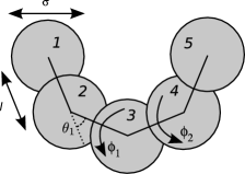
Figure 3: A cartoon of the model. Five monomers are shown, of diameter $\sigma$, bond length $l$, with bond angle $\theta_{1}$ and the two dihedral angles $\phi_{1}$ and $\phi_{2}$ indicated.

The position of monomer $i$ is denoted by $\mathbf{R}_{i}$. Bond vectors are defined as $\mathbf{r}_{i}=\mathbf{R}_{i+1}-\mathbf{R}_{i}$. Separation between monomers $i$ and $j$ is denoted $r_{ij}$. The bond angle around monomer $i$ is defined as the angle between bond $\mathbf{r}_{i-1}$ and $\mathbf{r}_{i}$, that is $\cos\theta_{i}=\mathbf{r}_{i-1}\cdot\mathbf{r}_{i}$. The dihedral (torsional) angle $\phi_{i}$ is defined as the angle between the planes formed by the vector pairs $\left(\mathbf{r}_{i-1},\mathbf{r}_{i}\right)$ and $\left(\mathbf{r}_{i},\mathbf{r}_{i+1}\right)$, relative to the cis conformation (i.e. $\phi=0$ is cis, $\phi=\pi$ is trans). We take positive $\phi$ as a right-handed rotation. This is, however, arbitrary, as the underlying model is achiral. We do not consider translations and rotations of the entire molecule; as such, we fix the position of the first monomer, as well as the plane made by the vectors $\mathbf{r}_{1}$ and $\mathbf{r}_{2}$. The configurational integral of such an n-mer is given by $\mathcal{Z}_{n}$, defined as:

$$\mathcal{Z}_{n} = \left(\prod_{i=1}^{n-3}\int_{-\pi}^{\pi}d\phi_{i}\right)\left(\prod_{j=1}^{n-2}\int_{0}^{\pi}l^{2}\sin\theta_{i}d\theta_{i}\right)\times$$ (2)

$$\quad\exp\left(-\beta E\left(\left\{\mathbf{R}_{i}\right\}\right)\right)$$

where $E\left(\left\{\mathbf{R}_{i}\right\}\right)$ is the total configurational energy for the system (the sum of the pairwise interactions as Eq. 1) and $\beta=1/k_{B}T$, the inverse temperature.

III.1 Tetramer

We initially consider a tetramer. The configurational integral is given by:

$$\mathcal{Z}_{4} = l^{4}\int_{-\pi}^{\pi}d\phi_{1}\int_{0}^{\pi}\sin\theta_{1}d\theta_{1}\int_{0}^{\pi}\sin\theta_{2}d\theta_{2}\times$$ (3)

$$\quad\exp\left(-\beta\left(u\left(r_{13}\right)+u\left(r_{24}\right)+u\left(r_{14}\right)\right)\right)$$

Separations are given by:

$$\begin{array}[]{ccc}r_{i-1,i+1}^{2}&=&2l^{2}\left(1+\cos\theta_{i}\right)\\ &=&l^{2}x_{i}\end{array}$$ (4)

and

$$\begin{array}[]{ccl}r_{i-1,i+2}^{2}\left(\theta_{i},\theta_{i+1},\phi_{i}\right)&=&l^{2}\left(\left(1+\cos\theta_{i}+\cos\theta_{i+1}\right)^{2}\right.\\ &&\qquad+\sin^{2}\theta_{i}+\sin^{2}\theta_{i+1}\\ &&\qquad\left.-2\sin\theta_{i}\sin\theta_{i+1}\cos\phi_{i}\vphantom{\left(\theta\right)^{2}}\right)\\ &=&l^{2}\left(\left(x_{i}+x_{i+1}-2\right)^{2}/4\right.\\ &&\qquad+x_{i}\left(4-x_{i}\right)/4\\ &&\qquad+x_{i+1}\left(4-x_{i+1}\right)/4\\ &&\qquad-\cos\phi_{i}\sqrt{x_{i}\left(4-x_{i}\right)}\times\\ &&\qquad\left.\sqrt{x_{i+1}\left(4-x_{i+1}\right)}/2\right)\\ &=&l^{2}y_{i}\left(x_{i},x_{i+1},\phi_{i}\right)\end{array}$$ (5)

Since we are working with variables of squared separation, for notational convenience we also define $a=\left(\sigma/l\right)^{2}$. Physical bounds for $x_{i}$ are $a\leq x_{i}\leq 4$, since a separation of less than $\sigma$ represents an overlap. It is natural to switch variables in the configurational integral to separations $x_{i}$, giving:

$$\mathcal{Z}_{4} = (1/4)\int_{-\pi}^{\pi}d\phi_{1}\int_{0}^{4}dx_{1}\int_{0}^{4}dx_{2}\times$$ (6)

$$\quad\exp\left(\vphantom{\left(\sqrt{\phi}\right)}-\beta\left(u\left(l\sqrt{x_{1}}\right)+u\left(l\sqrt{x_{2}}\right)\right.\right.$$

$$\qquad\left.\left.+u\left(l\sqrt{y_{1}\left(x_{1},x_{2},\phi_{1}\right)}\right)\right)\right)$$

Since we are working in a square-well system with discretized energies, it is now convenient to switch to a density-of-states representation:

$$\mathcal{Z}_{4}=\left(1/4\right)\sum_{k=0}^{3}\omega_{4}(k)\exp(\beta\epsilon k)$$ (7)

where $\omega_{n}(k)$ is the density of states for the n-mer with $k$ contacts. For the tetramer, we can write the appropriate integrals:

$$\omega_{4}(0) = \int d\phi_{1}\int_{\min(4,\lambda^{2}a)}^{4}dx_{1}\int_{\min(4,\lambda^{2}a)}^{4}dx_{2}\times$$ (8)

$$\quad\Theta\left(y_{1}\left(x_{1},x_{2},\phi_{1}\right)-\lambda^{2}a\right)$$

$$\omega_{4}(1) = 2\int_{-\pi}^{\pi}d\phi_{1}\int_{\min(4,\lambda^{2}a)}^{4}dx_{1}\int_{a}^{\min(4,\lambda^{2}a)}dx_{2}\times$$ (9)

$$\quad\Theta\left(y_{1}\left(x_{1},x_{2},\phi_{1}\right)-\lambda^{2}a\right)$$

$$+\int_{-\pi}^{\pi}d\phi_{1}\int_{\min(4,\lambda^{2}a)}^{4}dx_{1}\int_{\min(4,\lambda^{2}a)}^{4}dx_{2}\times$$

$$\quad\left[\Theta\left(y_{1}\left(x_{1},x_{2},\phi_{1}\right)-a\right)\right.$$

$$\qquad\left.-\Theta\left(y_{1}\left(x_{1},x_{2},\phi_{1}\right)-\lambda^{2}a\right)\right]$$

$$\omega_{4}(2) = 2\int_{-\pi}^{\pi}d\phi_{1}\int_{\min(4,\lambda^{2}a)}^{4}dx_{1}\int_{a}^{\min(4,\lambda^{2}a)}dx_{2}\times$$ (10)

$$\quad\left[\Theta\left(y_{1}\left(x_{1},x_{2},\phi_{1}\right)-a\right)\right.$$

$$\qquad-\left.\Theta\left(y_{1}\left(x_{1},x_{2},\phi_{1}\right)-\lambda^{2}a\right)\right]$$

$$+\int_{-\pi}^{\pi}d\phi_{1}\int_{a}^{\min(4,\lambda^{2}a)}dx_{1}\int_{a}^{\min(4,\lambda^{2}a)}dx_{2}\times$$

$$\quad\Theta\left(y_{1}\left(x_{1},x_{2},\phi_{1}\right)-\lambda^{2}a\right)$$

$$\omega_{4}(3) = \int_{-\pi}^{\pi}d\phi_{1}\int_{a}^{\min(4,\lambda^{2}a)}dx_{1}\int_{a}^{\min(4,\lambda^{2}a)}dx_{2}\times$$ (11)

$$\quad\left[\Theta\left(y_{1}\left(x_{1},x_{2},\phi_{1}\right)-a\right)\right.$$

$$\qquad\left.-\Theta\left(y\left(x_{1},x_{2},\phi_{1}\right)-\lambda^{2}a\right)\right]$$

where $\Theta\left(x\right)$ is the Heaviside step function. The min terms exist to prevent unphysical limits of integration when $\lambda^{2}a\geq 4$ (in which case 1-3 contacts are “always on”). We note that $\omega_{4}(k)$ is a sum of integrals of the general form:

$$f_{4}=2\int_{0}^{\pi}d\phi_{1}\int_{x_{1l}}^{x_{1h}}dx_{1}\int_{x_{2l}}^{x_{2h}}dx_{2}\Theta\left(y_{1}\left(x_{1},x_{2}\phi_{1}\right)-h\right)$$ (12)

where we have used the symmetry of the system to simplify the $\phi_{1}$ integral. The integrand is non-zero for that region of $\left(x_{1},x_{2},\phi_{1}\right)$ space for which $y_{1}>h$. We can solve Eq. (5) to find the bound of this space with respect to $x_{2}$ (or, by symmetry, $x_{1}$) for given $(\phi,h)$, which we call $x_{c}$:

$$x_{c}\left(x,\phi,h\right) = 2\left(\vphantom{\sqrt{\left(h\right)^{2}}}x\left(t\left(4-x\right)+\left(h-1\right)\right)\right.$$ (13)

$$\quad+\mathrm{sgn(\cos(\phi_{1}))}\sqrt{t\left(4-x\right)x}\times$$

$$\quad\left.\sqrt{\left(2x\left(2t+h-1\right)-tx^{2}-\left(h-1\right)^{2}\right)}\right)$$

$$/\left(x\left(x+t\left(4-x\right)\right)\right)$$

where we use $t=\cos^{2}\phi$, and $\mathrm{sgn}(x)$ returns the sign of $x$. Similarly, we also solve for the value of $\phi$ at which $y_{i}=h$ for given $x_{i}$ and $x_{i+1}$, which we denote $\phi_{c}$:

$$\phi_{c}\left(x_{i},x_{i+1},h\right)=\begin{cases}\pi&\Phi<-1\\ \arccos\left({\displaystyle\Phi}\right)&\left|\Phi\right|<1\\ 0&\Phi>1\end{cases}$$ (14)

where the ratio $\Phi$ is defined as:

$$\Phi={\displaystyle\frac{2+x_{i}x_{i+1}-2h}{\sqrt{x_{i}\left(4-x_{i}\right)x_{i+1}\left(4-x_{i+1}\right)}}}$$ (15)

We consider the shape of this boundary:

$$\left.\frac{\partial\phi_{c}}{\partial x_{i}}\right|_{x_{i+1}} = \frac{2\sqrt{x_{i+1}\left(4-x_{i+1}\right)}}{\sin\phi_{c}\sqrt{x_{i}\left(4-x_{i}\right)}}\times$$ (16)

$$\quad\left(2(1-h)-x_{i}\left(x_{i+1}+(1-h)\right)\right)$$

The only part of this equation which can be negative is the final bracket. Within the range $a\leq x_{i}\leq 4$, $a\leq h\leq\lambda^{2}a$, $1\leq a<4$ and $\lambda^{2}>1$, it can be shown that $\left.\frac{\partial\phi_{c}}{\partial x_{i}}\right|_{x_{i+1}}$ is non-positive. By symmetry, $\left.\frac{\partial x_{c}}{\partial x}\right|_{\phi}$ is therefore also non-positive. As such, we can write Eq. (12) as:

$$f_{4}=2\int_{0}^{\pi}d\phi_{1}\int_{x_{1l}}^{x_{1h}}dx_{1}\int_{\min\left(x_{2h},\max\left(x_{2l},x_{c}\left(x_{1},\phi,h\right)\right)\right)}^{x_{2h}}dx_{2}$$ (17)

The max term picks the larger of the original lower limit ($x_{2l}$) and the value of $x_{2}$ below which the Heaviside function integrand in Eq. (12) becomes zero. The min prevents the unphysical result of the lower limit becoming larger than than the upper limit.

We note that, by symmetry, if $x_{1}=x_{c}\left(x_{2},\phi,h\right)$, then $x_{2}=x_{c}\left(x_{1},\phi,h\right)$. Hence, we can immediately see that the solution to $x_{2h}=x_{c}\left(x_{1},\phi_{1},h\right)$ with respect to $x_{1}$ is $x_{1}=x_{c}\left(x_{2h},\phi,h\right)$. For $x_{1}<x_{c}\left(x_{2h},\phi,h\right)$, the upper and lower limits on the innermost integral are equal, and hence the contribution to the integral is zero, hence:

$$f_{4} = 2\int_{0}^{\pi}d\phi_{1}\int_{\min\left(x_{1h},\max\left(x_{1l},x_{c}\left(x_{2h},\phi,h\right)\right)\right)}^{x_{1h}}dx_{1}\times$$ (18)

$$\quad\int_{\max\left(x_{2l},x_{c}\left(x_{1},\phi,h\right)\right)}^{x_{2h}}dx_{2}$$

Since $x_{c}\left(x,\phi,h\right)$ is a monotonically decreasing function of $x$ across the range of interest, we can now propagate the max term in the middle integral out to the dihedral integral:

$$f_{4} = 2\int_{\phi_{c}\left(x_{1l},x_{2h},h\right)}^{\pi}d\phi_{1}\int_{x_{1l}}^{x_{1h}}dx_{1}\times$$ (19)

$$\quad\int_{\max\left(x_{2l},x_{c}\left(x_{1},\phi,h\right)\right)}^{x_{2h}}dx_{2}$$

$$+2\int_{0}^{\phi_{c}\left(x_{1l},x_{2h},h\right)}d\phi_{1}\int_{\min\left(x_{1h},x_{c}\left(x_{2h},\phi,h\right)\right)}^{x_{1h}}dx_{1}\times$$

$$\quad\int_{\max\left(x_{2l},x_{c}\left(x_{1},\phi,h\right)\right)}^{x_{2h}}dx_{2}$$

The remaining max and min terms can then be propagated out in a similar fashion, remembering that $\phi_{c}\left(x,x^{\prime},h\right)$ is a monotonically decreasing function of $x$ and $x^{\prime}$ across the range of interest:

$$\begin{array}[]{l}f_{4}=2\int_{\phi_{c}\left(x_{1l},x_{2l}\right)}^{\pi}d\phi_{1}\int_{x_{1l}}^{x_{1h}}dx_{1}\int_{x_{2l}}^{x_{2h}}dx_{2}\\ +2\int_{\max\left(\phi_{c}\left(x_{1l},x_{2h}\right),\phi_{c}\left(x_{1h},x_{2l}\right)\right)}^{\phi_{c}\left(x_{1l},x_{2l}\right)}d\phi_{1}\int_{x_{c}\left(x_{2l}\right)}^{x_{1h}}dx_{1}\int_{x_{2l}}^{x_{2h}}dx_{2}\\ +2\int_{\max\left(\phi_{c}\left(x_{1l},x_{2h}\right),\phi_{c}\left(x_{1h},x_{2l}\right)\right)}^{\phi_{c}\left(x_{1l},x_{2l}\right)}d\phi_{1}\int_{x_{1l}}^{x_{c}\left(x_{2l}\right)}dx_{1}\int_{x_{c}}^{x_{2h}}dx_{2}\\ +2\int_{\phi_{c}\left(x_{1l},x_{2h}\right)}^{\max\left(\phi_{c}\left(x_{1l},x_{2h}\right),\phi_{c}\left(x_{1h},x_{2l}\right)\right)}d\phi_{1}\int_{x_{1l}}^{x_{1h}}dx_{1}\int_{x_{c}}^{x_{2h}}dx_{2}\\ +2\int_{\min\left(\phi_{c}\left(x_{1l},x_{2h}\right),\phi_{c}\left(x_{1h},x_{2l}\right)\right)}^{\phi_{c}\left(x_{1l},x_{2h}\right)}d\phi_{1}\int_{x_{c}\left(x_{2l}\right)}^{x_{1h}}dx_{1}\int_{x_{2l}}^{x_{2h}}dx_{2}\\ +2\int_{\min\left(\phi_{c}\left(x_{1l},x_{2h}\right),\phi_{c}\left(x_{1h},x_{2l}\right)\right)}^{\phi_{c}\left(x_{1l},x_{2h}\right)}d\phi_{1}\int_{x_{c}\left(x_{2h}\right)}^{x_{c}\left(x_{2l}\right)}dx_{1}\int_{x_{c}}^{x_{2h}}dx_{2}\\ +2\int_{\phi_{c}\left(x_{1h},x_{2h}\right)}^{\min\left(\phi_{c}\left(x_{1l},x_{2h}\right),\phi_{c}\left(x_{1h},x_{2l}\right)\right)}d\phi_{1}\int_{x_{c}\left(x_{2h}\right)}^{x_{1h}}dx_{1}\int_{x_{c}}^{x_{2h}}dx_{2}\end{array}$$ (20)

For notational convenience, superfluous arguments to the functions $\phi_{c}$ and $x_{c}$ have been omitted; that is, $h$ and variables of integration. There are min and max terms in the dihedral integral since, without knowing more about the original limits $x_{il}$ and $x_{ih}$, it is not possible to tell whether $\phi_{c}\left(x_{1h},x_{2l},h\right)<\phi_{c}\left(x_{1l},x_{2h},l\right)$.

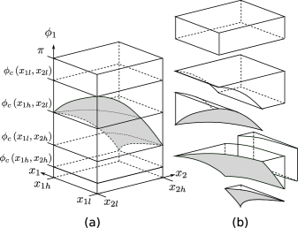
Figure 4: Graphical interpretation of the integrals in Eq. (20) when $\phi_{c}\left(x_{1h},x_{2l}\right)>\phi_{c}\left(x_{1l},x_{2h}\right)$. Part (a) shows the entire space in $x_{1},x_{2},\phi_{1}$; the total integral is the volume above the gray surface. Part (b) breaks the volume corresponding to the total integral into the parts listed in Eq. (20)

The first integral is trivial. The remaining integrals include a term $\int x_{c}(x_{1l},\phi_{1},h)d\phi_{1}$; this is analytically tractable, resulting in terms involving elliptic integrals, but is simpler to treat numerically. The final two terms include integrals of the form $\int\int x_{c}(x_{1},\phi_{1},h)dx_{1}d\phi$, which are not analytically tractable, and are thus treated numerically.

Calculation of the $f_{4}$ integrals via Eq. (20) allows calculation of the density of states via Eqs. (8 - 11), from which the equation of state and energy probability distributions can be determined. Structural information, in the form of the dihedral angle probability distributions, is also easily accessible. The dihedral density of states $g_{4}(\phi_{1},k)$ is given by integrals as Eqs. (8 - 11) without the integral over the dihedral angle. For the tetramer, these give tractable though lengthy analytic forms. The probability of observing a given dihedral angle is then given by:

$$P\left(\phi_{1};T\right)=\sum_{k=0}^{4}g_{4}\left(\phi_{1},k\right)\exp(\beta\epsilon k)/\mathcal{Z}_{4}$$ (21)

III.2 Pentamer

An equivalent procedure may be carried out for a pentamer. We first introduce the 1-5 separation, $z_{i}\left(x_{i},x_{i+1},x_{i+2},\phi_{i},\phi_{i+1}\right)=r_{i-1,i+3}^{2}/l^{2}$:

$$z_{i} = x_{i}+x_{i+2}-\sqrt{x_{i+1}\left(4-x_{i+1}\right)}\times$$ (22)

$$\quad\left(\cos\phi_{i}x_{i+2}\sqrt{x_{i}\left(4-x_{i}\right)}\right.$$

$$\qquad\left.\cos\phi_{i+1}x_{i}\sqrt{x_{i+2}\left(4-x_{i+2}\right)}\right)/4$$

$$+\left(x_{i+1}-2\right)\left(\vphantom{\sqrt{\left(x_{i}^{i}\right)}}x_{i}x_{i+2}-\cos\phi_{i}\cos\phi_{i+1}\times\right.$$

$$\qquad\left.\sqrt{x_{i}\left(4-x_{i}\right)x_{i+2}\left(4-x_{i+2}\right)}\right)/4$$

$$+\sin\phi_{i}\sin\phi_{i+1}\times$$

$$\quad\sqrt{x_{i}\left(4-x_{i}\right)x_{i+2}\left(4-x_{i+2}\right)}/2$$

where the arguments to $z_{i}$ have been omitted. The partition function for the pentamer is given by:

$$\mathcal{Z}_{5}=(1/8)\sum_{k=0}^{6}\omega_{5}(k)\exp(\beta\epsilon k)$$ (23)

Equivalent expressions to Eqs. (8-11) are simple to construct, using the equivalent form to Eq. (12):

$$f_{5} = 2\int_{0}^{\pi}d\phi_{1}\int_{-\pi}^{\pi}d\phi_{2}\int_{x_{1l}}^{x_{1h}}dx_{1}\int_{x_{2l}}^{x_{2h}}dx_{2}\int_{x_{3l}}^{x_{3h}}dx_{3}\times$$ (24)

$$\quad\Theta\left(y_{1}-h_{1}\right)\Theta\left(y_{2}-h_{2}\right)\Theta\left(z_{1}-h_{3}\right)$$

where we have suppressed the arguments of $y_{1}$, $y_{2}$ and $z_{1}$ for notational ease. This integral is constructed (without loss of generality) such that $\phi_{1}$ is always right-handed. Explicit bounds of integration due to 1-4 interactions can be treated in the same manner as for the tetramer case. Bounds for the $x_{1}$ and $x_{2}$ integrals as a function of $\phi_{1}$, and for the $x_{2}$ and $x_{3}$ integrals as a function of $\phi_{2}$, are determined exactly as Eq. (20). This leads to single ranges of integration for $x_{1}$ and $x_{3}$, and two sets of ranges of integration for $x_{2}$. The proper range of integration over $x_{2}$ is then the overlap of these two ranges. Explicitly treating the bounds of integration due to 1-5 interactions is not trivial, and as such the resulting integral is treated numerically. Dihedral probability distributions $P\left(\phi_{1},\phi_{2},T\right)$ can be calculated from dihedral densities of states $g_{5}\left(\phi_{1},\phi_{2},k\right)$ in an analogous manner to the tetramer.

IV Results

Using the results presented in Sec. III, we have evaluated the full partition functions for tetramers and pentamers. Results for the tetramer have been calculated with the Mathematica symbolic algebra package, using Gauss-Kronrod numerical integration. Results for the pentamer have been calculated using ten-point Gauss-Legendre quadrature (Press et al., 2002). Both methods of integration have been checked by comparison against the tangent chain results presented by Taylor (Taylor, 2003). The pentamer results have been verified against short Monte Carlo simulations (data not shown).

IV.1 Tetramer

To validate the method, we compare our calculated densities of states for tetramer tangent square well chains ($\sigma/l=1$) to those presented by Taylor (Taylor, 2003). These results are shown in Table 1.

Table 1: Comparison of the densities of states for a square well tetramer chain, $\sigma/l=1.0$ and $\lambda\sigma=1.5$ calculated in this work ($\omega_{4}(k)/4l^{4}$, with the factor $1/4$ (as described in section III) and by Taylor (Taylor, 2003) ($\omega_{4}^{(Taylor)}(k)$, or $g_{4}^{(k)}$ in the original terminology). Suppression of the unimportant multiplicative factor of $8\pi$ in the work of Taylor leads to the difference in the values; it can be seen that including this factor, the values differ only in the fourth and fifth significant figure.

$k$	$\omega_{4}(k)/4l^{4}$	$\omega_{4}^{(Taylor)}(k)$	$\omega_{4}(k)/\left(32\pi\omega_{4}^{(Taylor)}(k)\right)$
0	4.78131	0.19029	0.999750
1	5.59121	0.22247	0.999987
2	2.42528	0.09650	0.999986
3	0.62013	0.02467	1.000170

It can be seen that the results are equivalent to four significant figures aside from an unimportant multiplicative factor. The method of Taylor does not use explicit limits of integration, instead numerically integrating the Heaviside functions in Eq. (12); strictly, the method presented here should be more accurate, though these results suggest the difference is not significant.

The calculated densities of states as a function of $\sigma/l$ are shown in Fig. 5.

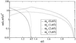
Figure 5: Densities of states for tetramers plotted against $\sigma/l$.

The densities of states for the $k=0$ and $k=1$ states are zero for $\sigma/l\geq 4/3$. For overlaps greater than this “magic number”, 1-3 interactions become “always on” — that is, $r_{i-1,i+1}\leq\lambda\sigma$ for all values of $\theta_{i}$ with $\lambda=3/2$. This also gives rise to a kink (discontinuity in the derivative) of $\omega_{4}(2,\sigma/l$). This is because at $\sigma/l=4/3$, the first term in Eq. (10) (which refers to the density of states for tetramers with a single 1-3 contact and a 1-4 contact) becomes zero, as the limits on the $x_{1}$ integral become equal.

As $\sigma/l\rightarrow 2$, the polymer becomes increasingly rigid, and the available conformational space vanishes. The calculated densities of states show the correct behavior at this limit.

Properties calculated from these densities of states are shown in Figs. 6 (energy) and 7 (heat capacity).

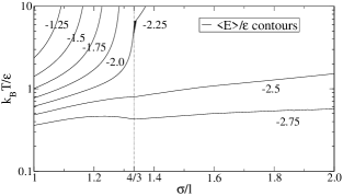
Figure 6: Ensemble average energies $\left\langle E\right\rangle/\epsilon$ for tetramers plotted against $\sigma/l$ and temperature $T$. Solid lines show energy contours at the labeled value. Note the discontinuities in the slope of the energy contours at $\sigma/l=4/3$ (shown by the dotted line).

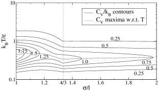
Figure 7: Configurational heat capacity $C_{V}$ for tetramers plotted against $\sigma/l$ and temperature. Solid lines show contours at the labeled value. The dashed line shows the line of maxima in $C_{V}$ with respect to temperature $T$. Note the discontinuities in the slope of the heat capacity contours at $\sigma/l=4/3$ (shown by the dotted line).

At $\sigma/l=4/3$, the slope of the energy and heat capacity contours show discontinuities in their derivatives. As such, the derivatives $\left(\partial U/\partial\sigma\right)_{T}$ and $\left(\partial C_{V}/\partial\sigma\right)_{T}$ have singularities at $\sigma/l=4/3$, however, these are not physically meaningful response functions. In simulated systems (Magee et al., 2006), bond lengths are not rigid, and bond length fluctuations will have the effect of “smoothing out” the discontinuity.

Though the tetramer does not show any other discontinuities, it does show a line of maxima in heat capacity with respect to temperature. We follow Taylor (Taylor, 2003) and Zhou, et al. (Zhou et al., 1997) in ascribing these maxima to collapse of the tetramer into compact conformations. The strength of these maxima can be seen to decrease with increase in $\sigma/l$. Further, the line of maxima shows re-entrance with respect to $\sigma/l$, with the temperature at which heat capacity is maximal itself having a maximum with respect to $\sigma/l$ at a point below $\sigma/l=4/3$.

Representative results for the torsional behavior of the tetramer are shown in Fig. 8,

Figure 8: Contour plots of $P\left(\phi_{1};T\right)$ for (a) $\sigma/l=1.0$, (b) $\sigma/l=1.3$, (c) $\sigma/l=1.6$ and (d) $\sigma/l=1.9$. Solid lines show contours at the labeled value. Dashed lines show maxima in $P\left(\phi_{1};T\right)$.

where we show the probability $P(\phi_{1};T)$ for four values of $\sigma/l$. At low values of the overlap ($\sigma/l\lesssim 1.48$), we see maxima in $P(\phi_{1};T)$ for non-zero $\phi_{1}$ at all temperatures, with the maxima becoming stronger and moving closer to zero (cis conformation) as temperature decreases. For intermediate values of overlap ($1.48\lesssim\sigma/l<\sqrt{(3+\sqrt{5})/2}$), weak maxima in $P(\phi_{1};T$) are seen for non-zero $\phi_{1}$ at high temperatures; however, the most probable conformation becomes $\phi_{1}=0$ (cis conformation) at low temperature. For large values of overlap ($\sigma/l>\sqrt{(3+\sqrt{5})/2}$), $P(\phi_{1};T)$ has only a single maximum at $\phi_{1}=0$ for all temperatures. The points separating the two regimes ($\max\left(P\left(\phi_{1};T\right)\right)=0$ and $\neq 0$) can be calculated analytically, as the points at which $\left.{\displaystyle\frac{\partial P(\phi_{1};T)}{\partial\phi_{1}}}\right|_{\phi_{1}=0}=0$. The calculated line in overlap-temperature space is shown in Fig. 9 (a)

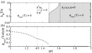
Figure 9: (a) Behavior of $P(\phi=0;T)$ with respect to $\sigma/l$; to the left of the solid line, $P(\phi=0)$ is a minimum, whilst to the right, $P(\phi=0)$ is a maximum. Directly on the line, $P(\phi=0)$ is a point of inflection. Dashed lines indicate the upper and lower bounds in $\sigma/l$ of the line. (b) The behavior of the maximum of $P(\phi_{1};T=0)$ (that is, in the ground state) with respect to $\sigma/l$. There is a kink in the line at $\sigma/l=4/3$, indicated by the dotted line.

. The upper limit of this line is the value of $\sigma/l$ at which $\phi_{c}\left(x_{i}=x_{i+1}=h=a\right)=0$. For values of overlap equal to or larger than this, it is not possible for the polymer to exhibit 1-4 overlaps, and there is no steric hindrance to $\phi_{1}=0$ states, which are the points of closest 1-4 approach. The lower limit of this region occurs at the point where the maximum of $P(\phi_{1};T=0)$ (see Fig. 9 (b)) becomes zero. The value of $\sigma/l$ at this limit does not admit a simple interpretation or expression.

IV.2 Pentamer

A comparison between the densities of states calculated here for pentamer tangent square well chains with those presented by Taylor is provided in Table 2.

Table 2: Comparison of the densities of states for a square well tetramer chain, $\sigma/l=1.0$ and $\lambda\sigma=1.5$ calculated in this work ($\omega_{5}(Ek)/4l^{4}$, with the factor $1/4$ as described in section III) and by Taylor ($\omega_{5}^{(Taylor)}(k)$, or $g_{5}^{(k)}$ in the original terminology) . Suppression of an unimportant multiplicative factor of $16\pi^{2}$ in the work of Taylor leads to the difference in the values; it can be seen that including this factor, the differences in the values are negligible.

k	$\omega_{5}(k)/4l^{4}$	$\omega_{4}^{(Taylor)}(k)$	$\omega_{4}(k)/\left(64\pi^{2}\omega_{4}^{(Taylor)}(k)\right)$
0	12.963393	0.08206	1.000386
1	21.368822	0.13531	1.000071
2	14.300928	0.09057	0.999908
3	7.300283	0.04626	0.999342
4	2.284838	0.01447	0.999924
5	0.0633290	0.004012	0.999590
6	0.035383	0.0002222	1.008395

Results are equivalent to four significant figures. The calculated densities of states as a function of $\sigma/l$ are shown in Fig. 10.

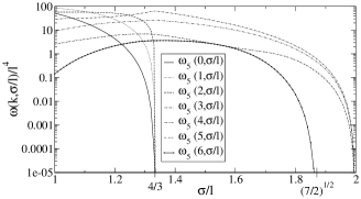
Figure 10: Densities of states for pentamers plotted against $\sigma/l$.

Once again, we see the highest energy densities of states going to zero at $\sigma/l=4/3$ as 1-3 interactions become “always on”, combined with a kink in the density of states for the highest remaining energy. All densities of states tend to zero as $\sigma/l\rightarrow 2$, where the available conformational space becomes zero. There are two further behaviors, not seen in the tetramer. The most obvious is that the density of the lowest energy state $\omega_{5}(6)$ becomes zero at $\sigma/l=\sqrt{7/2}$. For values of overlap larger than this, the pentamer has become so stiff that it cannot bend back on itself far enough to make 1-5 contacts.

A further interesting behavior is observed at intermediate values of $\sigma/l$ where the ground state $\omega_{5}(6)$ becomes the same order of magnitude as $\omega_{5}(5$). Indeed, for $1.53\lesssim\sigma/l\lesssim 1.56$, $\omega_{5}(6)>\omega_{5}(5)$. This gives rise to a concavity in the entropy $S(k)=k_{B}\ln\omega(k)$ of the system with respect to energy at $E=-5\epsilon$, which can be studied using the discrete analog to the second derivative, $S^{\prime\prime}(k)=\left(S(k+1)-2S(k)+S(k-1)\right)$; the function is concave if $S^{\prime\prime}(k)$ is negative. The concavity results in a bimodal probability distribution function $P(E;T,\sigma/l)$ (illustrated in Fig. (11))

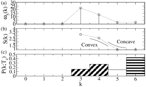
Figure 11: Concavity in the entropy and bimodal energy probability distribution for $\sigma/l=1.55$. (a) The density of states $\omega_{5}(k)$. (b) The entropy as a function of $k$; note the concavity at $k=5$. (c) The probability distribution function $P(k,T)$ at the “state coexistence” temperature. The function is bimodal, and the total weights of the two “states” ($k<5$ (diagonal shading) and $k>5$ (horizontal shading)) are equal. Dashed lines serve as a guide to the eye.

. In analogy to the study of phase transitions, we find the line of temperatures at which the two peaks of these bimodal probability distributions have equal weight - a line of “state coexistence”. This line is plotted alongside the data in Figs. 12 (energy)

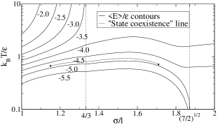
Figure 12: Ensemble average energies $\left\langle E\right\rangle/\epsilon$ for pentamers plotted against $\sigma/l$ and temperature $T$. Solid lines show energy contours at the labeled value. The dashed line shows the “state coexistence” line. Note the discontinuities in the slope of the energy contours at $\sigma/l=4/3$ and $\sigma/l=\sqrt{7/2}$(shown by dotted lines).

and 13 (heat capacity),

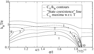
Figure 13: Configurational heat capacity $C_{V}$ for pentamers plotted against $\sigma/l$ and temperature. Solid lines show contours at the labeled value. The dashed line shows the line of maxima in $C_{V}$ with respect to temperature $T$. The dot-dashed line shows the “state coexistence” line — the position of the end points of this line near a contour line is purely coincidental. Note the discontinuities in the slope of the heat capacity contours at $\sigma/l=4/3$ and $\sigma/l=\sqrt{7/2}$ (shown by dotted lines).

and runs from $\sigma/l\approx 1.14$ to $\sigma/l\approx 1.72$. These end points are at non-zero temperature, and occur where the curvature of the free energy at $E=-5\epsilon$ becomes zero. The end points are not associated with heat capacity divergences.

The thermodynamic data shows the expected discontinuities in the slope of energy and heat capacity contour at the “magic numbers” $\sigma/l=4/3$ and $\sigma/l=\sqrt{7/2}$. The lower magic number corresponds to the loss of high energy states, as for the tetramer. The larger magic number, corresponding to the loss of the $k=6$ state, gives a discontinuity in the energy at zero temperature (from $E=-6\epsilon$ to $E=-5\epsilon$). As for the tetramer, bond length fluctuations in real systems would act to smooth out these discontinuities in real systems.

The pentamer also shows a line of heat capacity maxima, which lies at lower temperature than the “state coexistence” line. Both these lines show a discontinuity in slope at $\sigma/l=4/3$. Both lines are doubly reentrant, showing one maximum below $\sigma/l=4/3$, and another above $\sigma/l=4/3$. The line of heat capacity maxima connects with the discontinuity in energy at $\sigma/l=\sqrt{7/2}$.

The dihedral behavior of the pentamer at zero temperature (ground state) is shown in Fig. 14,

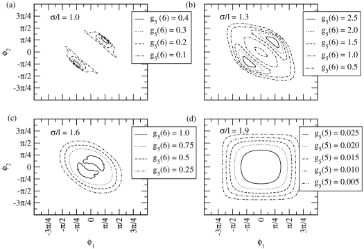
Figure 14: Ground state dihedral densities of states $g_{5}\left(\phi_{1},\phi_{2},6\right)$ for (a) $\sigma/l=1.0$, (b) $\sigma/l=1.3$, and (c) $\sigma/l=1.6$, and (d) $g_{5}\left(\phi_{1},\phi_{2},5\right)$ for $\sigma/l=1.9$; the ground state is $-5\epsilon$ for $\sigma/l=1.9$. Lines show contours as denoted in figure legends.

in four representative plots of the ground state dihedral densities of states $g_{5}\left(\phi_{1},\phi_{2},6\right)$ and $g_{5}\left(\phi_{1},\phi_{2},5\right)$. These are equivalent to unnormalized dihedral probability distributions for the system at $T=0$. We see that, for the three lowest values of $\sigma/l$, the probabilities are peaked at points on the $\phi_{1}=\phi_{2}$ diagonal; the dihedrals prefer to take the same sign. This continues to the “magic number” $\sigma/l=\sqrt{(3+\sqrt{5})/2}$, where, as for the tetramer, 1-4 overlaps can no longer occur, and steric effects no longer prevent cis conformations. As the degree of overlap tends to this number, and the amount of steric interference decreases, the maxima move closer to $\phi_{1}=\phi_{2}=0$. For $\sigma/l\geq\sqrt{(3+\sqrt{5})/2}$, the probability distributions become unimodal at $\phi_{1}=\phi_{2}=0$. This should be compared with the behavior for the tetramer (see Fig. 9), where $\phi_{max}(T=0)$ is zero for $\sigma/l\gtrsim 1.48$; this effect is due to the additional steric interference from 1-5 overlaps.

V Discussion and Conclusions

In the previous section, it has been shown that the tetramer and pentamer show a rich and surprising range of behaviors. Specifically, these are “magic numbers” of the overlap $\sigma/l$ where the derivatives of the densities of states change discontinuously, maxima in specific heat with respect to temperature, and a region of bimodal energy probability distributions, reminiscent of a first-order transition in bulk systems. In general, the behavior of long polymer chains cannot be directly inferred from the behavior of very short chains such as those studied in this work. If, however, interactions between monomers widely spaced along a chain can be neglected, the behavior of very short chains can be used as a basis for a spin chain model. Such interactions may be neglected when chains become very stiff (at, for e.g., large values of $\sigma/l$, or after helix formation). In this case, the behavior of the very short chains may be considered the “building block” for the behavior of longer chains.

The “magic numbers” which are observed correspond to discontinuous changes in the derivatives of the densities of states. At $\sigma/l=4/3$, 1-3 contacts become “always on” and high energy densities of states become zero. At $\sigma/l=\sqrt{(3+\sqrt{5})/2}$, the chain becomes so stiff that it cannot bend back upon itself far enough for 1-4 overlaps to occur. Similarly, at $\sigma/l=\sqrt{7/2}$, the chain becomes so stiff that 1-5 contacts can no longer occur, and the ground state for the pentamer is lost. These discontinuities in the densities of states are associated with discontinuities in the energy and compressibility with respect to the parameter $\sigma$. The “magic numbers” are similar in principle to the “cut-off” $\lambda$ values noted by Taylor (Taylor, 2003) for tangent chains — this work has not examined the effects of changing the well width parameter $\lambda$, but it is obvious that the values of these “magic numbers” will depend upon that parameter, and that “cut-off” values of $\lambda$ will also exist for this model. As has been noted above, the discontinuities across lines of constant $\sigma/l$ in this system will be smoothed in simulations with variable bond length, however, the effects should still be visible. We particularly note the sudden loss of stability of the “helix 1” phase at $\sigma/l\approx 1.675$ in previous simulation work (Magee et al., 2006) (see Fig. 1). Given the 10% bond length fluctuation allowed in those simulations, this loss of stability may coincide with the magic number at $\sigma/l=\sqrt{(3+\sqrt{5})/2}\approx 1.618$, suggesting that the more tightly wound “helix 1” phase is stabilized by steric interference of 1-4 contacts. This supposition is supported by the observed loss of double-peaked dihedral angle probability distributions for overlaps above this “magic number”, suggesting that the more loosely wound “helix 2” phase is stabilized by steric interference between monomers spaced further along the chain.

The low temperature maxima in the specific heat for these short polymers appear to be a continuation of the specific heat maxima observed for short tangent chains (Zhou et al., 1997; Taylor, 2003). We follow these previous works in interpreting these maxima as signatures of collapse to close-packed, low energy conformations. This interpretation appears confirmed by the presence of bimodal energy probability distributions for the pentamer, with a line of “state coexistence” which roughly parallels the line of maxima.

For the tetramer, the line of specific heat maxima shows re-entrance below $\sigma/l=4/3$, having a maximum with respect to temperature. For the pentamer, both the line of specific heat maxima and of “state coexistence” are doubly reentrant, showing maxima below and above $\sigma/l=4/3$. The re-entrance of the “state coexistence” line can be easily explained by reference to the densities of states shown in Fig. 10. Consider the system for $\sigma/l\geq 4/3$. For overlaps just above this point, the ground state density of states (the entropy of the low energy state) is increasing while all other densities of states are decreasing with increasing overlap. Hence, the low energy state becomes more stable, and coexistence moves to higher temperature. The ground state density of states soon begins to decrease, but as long as it is decreasing more slowly than the higher energy density of states, its stability continues to increase. However, on closer approach to $\sigma/l=\sqrt{7/2}$, the ground state density of states decreases faster than the higher energy densities of states, and stability decreases. The same argument holds for the line when $\sigma/l<4/3$. If we interpret the maximum in heat capacity as a result of structural competition between the ground state and higher energy states (following Stanley, et al. (Stanley et al., 1998)), we can make the same argument for the re-entrance in the lines of maxima for both the tetramer and pentamer. Physically, increasing the overlap of the chain makes configurations with lower energy (more contacts) more likely at first (as monomers are “drawn into” each other’s square wells), but then begins to cut into these low energy states as the chain becomes too stiff to bend back upon itself and make contacts. We attribute the re-entrance of the stability of the “helix 1” phase in previous work to this same competition between effects.

Though it seems reasonable to attribute the behavior of the phase boundary between the “helix 1” and globule phases to effects seen in the pentamer, it should be noted that the state coexistence seen in the pentamer is represents collapse of the pentamer, rather than helix formation. Though the dihedral probability distributions shown in Fig. 14 do show double peaks at non-zero dihedral angles, this is not a sufficient criterion for helicity. The cross-correlation coefficient of these distributions is not significantly above zero; the total statistical weight associated with dihedrals away from the peaks is still large enough to outweigh the correlated peaks. However, the clear double peaked structure does suggest that the physics necessary for helix formation is contained in these simple, small systems, particularly in the steric interference due to 1-4 overlaps.

While these results appear to clarify certain behaviors observed in simulations, they do raise further questions. Under the interpretation we have offered here, the nature of the “helix-2” phase is unclear; this phase is observed to be stable up to $\sigma/l=1.9$ in simulation (Magee et al., 2006), where the chain is too stiff for 1-5 overlaps to be the root of the observed chirality. Further, the question of how the helix transition connects (or does not connect) to the crystallization-like transition observed in simulations for the tangent chain system remains unresolved. Follow-up work, developing a spin chain model for helix formation using the results presented here, is underway; it is hoped that this approach will shed light upon these questions.