Chemical Analysis of Five Red Giants in the Globular Cluster M10 (NGC 6254)

Abstract

We have determined Al, $\alpha$, Fe–peak, and neutron capture elemental abundances for five red giant branch (RGB) stars in the Galactic globular cluster M10. Abundances were determined using equivalent width analyses of moderate resolution (R$\sim$15,000) spectra obtained with the Hydra multifiber positioner and bench spectrograph on the WIYN telescope. The data sample the upper RGB from the luminosity level near the horizontal branch to about 0.5 mag below the RGB tip. We find in agreement with previous studies that M10 is moderately metal–poor with [Fe/H]=–1.45 ($\sigma$=0.04). All stars appear enhanced in Al with $\langle$[Al/Fe]$\rangle$=+0.33 ($\sigma$=0.19), but no stars have [Al/Fe]$\gtrsim$+0.55. We find the $\alpha$ elements to be enhanced by +0.20 to +0.40 dex and the Fe–peak elements to have [el/Fe]$\sim$0, which are consistent with predictions from type II SNe ejecta. Additionally, the cluster appears to be r–process rich with $\langle$[Eu/La]$\rangle$=+0.41.

1 INTRODUCTION

Although few chemical analysis studies of M10 exist, the general consensus is that this cluster exhibits all of the classical characteristics observed in other Galactic globular clusters. With a metallicity of [Fe/H]$\approx$–1.5 (Kraft et al. 1995), M10 lies near the median metallicity distribution for halo globular clusters (Laird et al. 1988). Small sample (N$\lesssim$15) analyses of red giant branch (RGB) stars in this cluster have revealed it to have [$\alpha$/Fe]$\sim$+0.30 and [el/Fe]$\sim$0 for Fe–peak elements (Kraft et al. 1995; Mishenina et al. 2003). These values are consistent with the current generation of M10 stars having been polluted by the ejecta of type II supernovae (SNe) without significant contributions from type Ia SNe.

While it has long been known that nearly all globular cluster giants show star–to–star variations of the light elements (A$\lesssim$27), the source of many of these anomalies has yet to be determined. Numerous observations of globular cluster stars from the main sequence to above the RGB luminosity bump have revealed declining [C/Fe] and increasing [N/Fe] ratios as a function of increasing luminosity (e.g., see reviews by Kraft et al. 1994; Gratton et al. 2004; Carretta 2008). These observations show clear evidence of CN–cycle products being brought to the surface and are a confirmation of first dredge–up predictions (Iben 1964). Smith & Fulbright (1997) and Smith et al. (2005) have verified this trend in M10 as well as a CN band anticorrelation with [O/Fe] for stars at various RGB luminosities. However, the large spread in [N/Fe] of about 1.0 dex found by Smith et al. (2005) in M10 stars may be evidence for primordial variations superimposed on in situ mixing.

The C and N abundance anomalies are known to exist in both globular cluster and field giants, but that likeness does not extend to the well documented O/Na, Mg/Al, and O/F anticorrelations and Na/Al correlation seen solely in globular cluster stars (e.g., Gratton et al. 2004). These abundance relationships are clear signs of proton–capture nucleosynthesis, but where these processes are operating is still a mystery. Kraft et al. (1995) examined the O/Na anticorrelations of 15 bright giants in M10 along with M3 and M13, which are all globular clusters of similar metallicity ([Fe/H]$\approx$–1.5), because M10 and M13 have extremely blue horizontal branches (HB) but M3 has a uniform distribution of blue HB, RR Lyrae, and red HB stars. The study showed that M10 appears to be an intermediate case in terms of O depletion and Na enhancement in that the average [O/Fe] is lower in M10 than in M3, but no M10 giants were super O–poor (i.e., [O/Fe]$<$–0.6), suggesting the process driving O depletion does not itself determine HB morphology.

In this paper we have examined five additional RGB stars in M10 that are located above the luminosity of the horizontal branch but below the RGB tip. We have derived Al, $\alpha$, Fe–peak, and heavy element abundances to examine how M10 fits into context with other globular clusters of similar metallicity and HB morphology.

2 OBSERVATIONS AND REDUCTIONS

The observation of cluster giants were obtained using the Hydra multifiber positioner and bench spectrograph on the 3.5 meter WIYN telescope at Kitt Peak National Observatory in May, 2000. The observations consisted of three, 3,000 second exposures with the 200 $\mu$m red fiber bundle. The 316 line mm^-1 echelle grating and red camera provided a resolution of R ($\lambda$/$\Delta$$\lambda$)$\sim$15,000 at 6650 Å, with wavelength coverage extending from approximately 6460–6860 Å.

Target stars and photometry were taken from the photometric survey by Arp (1955) and astrometry was taken from the USNO Image and Catalogue Archive. Sample selection focused on observing stars with V magnitudes brighter than the HB and extending up to the RGB tip. However, the final sample only includes stars with magnitudes up to about 0.5 mag below the RGB tip. The Hydra configuration allowed for fiber placement on 22 objects, but only 7 of those 22 had sufficient signal–to–noise (S/N) for reliable abundance determinations. Two of the remaining program stars (IV–44 & IV–87) were found to have wavelength shifts and H$\alpha$ profiles inconsistent with being both cluster members and low surface gravity RGB stars. Comparison with the proper motion study by Chen et al. (2000) reveals that both of these stars have proper motions inconsistent with other cluster members.

The IRAF task ccdproc was used to trim the bias overscan region and apply the bias level correction. The IRAF routine dohydra was employed to apply the flat field correction, linearize the wavelength scale, correct for scattered light, remove cosmic rays, subtract the sky, and extract the one–dimensional spectra. Typical S/N ratios of individual spectra are 25–50 with co–added spectra having S/N ratios of about 50–75. A sample spectral region for all five program stars is shown in Figure 1.

3 ANALYSIS

3.1 Model Stellar Atmospheres

The significant differential reddening associated with M10 (e.g., von Braun et al. 2002) makes effective temperature (T_eff) and surface gravity (log g) estimates based on color and photometric indices difficult. Therefore, we employed an iterative method to obtain T_eff by removing Fe I abundance trends as a function of excitation potential and microturbulence (V_t) by removing Fe I abundance trends as a function of reduced width [log(EW/$\lambda$)]. Surface gravity was obtained by enforcing ionization equilibrium between Fe I and Fe II because ionized Fe lines in these cool giants are more sensitive to changes in log g than neutral lines (e.g., Johnson & Pilachowksi 2006; their Table 3). Despite the fact that only one Fe II line (6516 Å) was available for analysis, we used the ionization equilibrium method because of the potentially large and variable uncertainties in determining bolometric absolute magnitudes.

All initial models assumed a metallicity of [Fe/H] = –1.50, which is consistent with previous spectroscopic [Fe/H] estimates (e.g., Kraft et al. 1995; Mishenina et al. 2003). The model stellar atmospheres (without convective overshoot) were created by interpolating in the ATLAS grid (Castelli et al. 1997). The temperature range of our observations covers 4450 $\leq$ T_eff $\leq$ 4750 corresponding to surface gravity values of about 1.20 $\leq$ log g $\leq$ 1.85. Our adopted values of T_eff and log g are in reasonable agreement with position on the color–magnitude diagram as estimated from V and B–V photometry. A summary of our adopted model atmosphere parameters and associated photometry is provided in Table 1.

3.2 Equivalent Width Analyses

All abundances were determined by measuring equivalent widths using the splot package in IRAF. Given the moderate resolution and S/N of our spectra, we restricted measurements to isolated lines that did not suffer significant blending problems and which had equivalent widths $\gtrsim$10 mÅ. Suitable lines were chosen via comparison with a high S/N, high resolution Arcturus spectrum, which also served as a reference aiding continuum placement. The final linelist including all measured equivalent widths is given in Table 2, with atomic parameters taken from Johnson & Pilachowski (2006).

While most abundances were calculated using the abfind driver in the 2002 version of the LTE line analysis code MOOG (Sneden 1973), the elements Sc and Eu required a modified approach. These spectral features may be sensitive to hyper–fine splitting resulting from spin–orbit coupling and Eu has the added complication of having two naturally occurring stable isotopes (¹⁵¹Eu and ¹⁵³Eu). Both of these effects can cause line broadening that will force single–line equivalent width measurements to overestimate the abundances. Therefore, we used the blends driver in MOOG with linelists including hyperfine and/or isotopic data from Prochaska & McWilliam (2000) for Sc and C. Sneden (private communication, 2006) for Eu. While the 6774 Å La II line may also be sensitive to hyper–fine splitting, no known linelist exists in the literature for this transition. However, the typically small equivalent widths of this line ($\lesssim$30 mÅ) suggest additional broadening will not affect La abundances too severely.

4 RESULTS AND DISCUSSION

4.1 Al Abundances

We have determined at least upper limits of [Al/Fe] for five giants with the cluster having $\langle$[Al/Fe]$\rangle$=+0.33 ($\sigma$=0.19) and a full range of 0.50 dex. Both the star–to–star dispersion and average [Al/Fe] ratios are in agreement with observations of other Galactic globular clusters of similar metallicity (e.g., Kraft et al. 1998; Sneden et al. 2004; Cohen & Meléndez 2005; Johnson et al. 2005; Yong et al. 2005); however, the highest [Al/Fe] ratio found in our sample is about a factor of three smaller than the $>$+1.0 dex ratios observed in M3 and M13 (Pilachowski et al. 1996; Sneden et al. 2004; Johnson et al. 2005; Cohen & Meléndez 2005), which possess similar metallicity and, in the case of M13, a similar HB morphology. This may be due to our small sample size coupled with observations of stars well below the RGB tip, where additional Al enhancement due to extra in situ mixing may be operating (e.g., Denissenkov & VandenBerg 2003). Kraft et al. (1995) found M10 to be an intermediate case between M3 and M13 with regard to the amount of O depletion and Na enhancement and therefore given the likely Na–Al correlation present in this cluster one would not expect [Al/Fe] values much greater than about +0.80 dex. A complete list of our determined abundances for Al and all other elements is provided in Table 3.

It has been shown that [Fe/H] determinations based on Fe I lines in metal–poor stars suffer from larger LTE departure effects than their metal–rich counterparts because of overionization due to decreased UV line blocking (e.g., see review by Asplund 2005). Correcting for this effect would drive the [Fe/H] abundance up, perhaps by as much as $\sim$+0.30 dex at [Fe/H]=–3 (Thévenin & Idiart 1999, but see also Gratton et al. 1999; Kraft & Ivans 2003), and thus decrease the derived [Al/Fe] ratio found here. While a few NLTE studies for Al exist (e.g., Gehren et al. 2004; Andrievsky et al. 2008) finding offsets of order a few tenths of a dex, the actual Al NLTE correction for stars in the metallicity and luminosity regime studied here are mostly unknown. Fortunately, our sample does not vary widely in either metallicity or luminosity and any NLTE corrections are likely to be very similar, suggesting at least the relative star–to–star dispersion is a real effect.

In Figure 2 we compare abundances of various elements in M10 versus those in the similar cluster M12. The [Al/Fe] abundances for both clusters are comparable and each displays a modest star–to–star dispersion. Given that the scatter is about a factor of two larger than those observed in the Fe–peak and $\alpha$ elements, it is likely that the Al distribution is real and not an artifact of observational uncertainty. To see how M10 fits into the context of other Galactic globular clusters, we have plotted [Al/Fe] as a function of both horizontal branch ratio (HBR) and galactocentric distance (R_GC) for M10 and seven other clusters in Figure 3. The top panel suggests there is no significant relation between HBR and either the average [Al/Fe] ratio or the star–to–star dispersion. However, it should be noted that Carretta et al. (2007) do find a relationship between the extent of O/Mg depletions and Na/Al enhancements and the maximum temperature of stars located on the zero–age HB. The bottom panel may indicate a trend of increasing cluster average [Al/Fe] with increasing galactocentric distance; however, the sample size for each cluster varies between less than 10 to nearly 100 stars. Consequently, M10 does not appear to exhibit anomalous [Al/Fe] ratios compared to other globular clusters.

4.2 $\alpha$, Fe–Peak, and Heavy Elements

Nearly all globular clusters with [Fe/H]$<$–1 have [$\alpha$/Fe]$\sim$+0.30 to +0.50, solar Fe–peak to Fe ratios, and are r–process rich (e.g., Gratton et al. 2004). The star–to–star scatter present is usually $\lesssim$0.10 dex for the $\alpha$ and Fe–peak elements and $\sim$0.30–0.50 dex for the neutron capture elements, which is still significantly less than the 0.50–1.00 dex variations seen in light elements such as O, Na, and Al. In M10 we find the expected enhancement and small star–to–star dispersion of the two $\alpha$ elements Ca and Ti with $\langle$[Ca/Fe]$\rangle$=+0.42 ($\sigma$=0.12) and $\langle$[Ti/Fe]$\rangle$=+0.24 ($\sigma$=0.06). These values are consistent with the results from Kraft et al. (1995) that found $\langle$[Ca/Fe]$\rangle$=+0.29 ($\sigma$=0.07) and $\langle$[Ti/Fe]$\rangle$=+0.21 ($\sigma$=0.12) for a set of 10 other upper RGB stars in this cluster. The proxy Fe–peak elements Sc and Ni exhibit near solar abundance ratios in all stars with cluster average values of $\langle$[Sc/Fe]$\rangle$=+0.03 ($\sigma$=0.19) and $\langle$[Ni/Fe]$\rangle$=+0.09 ($\sigma$=0.06), which are roughly consistent with Kraft et al. (1995). These abundances patterns are mirrored in M12 (see Figure 2), but with M10 showing a smaller range of [Cr/Fe] and [Co/Fe] abundances. The combination of $\alpha$ enhancement and near solar Fe–peak ratios is consistent with this cluster being primarily polluted by the ejecta of type II SNe (e.g., Woosley & Weaver 1995).

For stars near M10’s metallicity, La is produced primarily via the s–process in $\sim$1–3 M_⊙ stars and Eu from the r–process in $\sim$8–10 M_⊙ stars (e.g., Busso et al. 1999; Truran et al. 2002). Our derived La and Eu abundances are consistent with the picture of massive stars producing most of the heavy elements in this cluster with $\langle$[La/Fe]$\rangle$=+0.08 ($\sigma$=0.29) and $\langle$[Eu/Fe]$\rangle$=+0.54 ($\sigma$=0.10). Comparing the ratio of r– to s–process elements gives [Eu/La]=+0.41 and implies M10 is slightly more r–process rich than the average globular cluster. However, this value is within the 1$\sigma$ range of $\langle$[Eu/Ba,La]$\rangle$=+0.23 ($\sigma$=0.21) found by Gratton et al. (2004) after combining data from the literature on 28 globular clusters. A larger sample size of M10 stars is likely to decrease the star–to–star scatter observed in our La and Eu sample but will probably not change the result that the cluster is r–process rich.

5 SUMMARY

We have determined abundances of the light element Al as well as several $\alpha$, Fe–peak, and heavy elements in five M10 red giants using moderate resolution spectroscopy (R$\sim$15,000) obtained with the Hydra multifiber spectrograph on the WIYN telescope. The data sample the upper RGB with luminosities ranging from above the level of the HB to about 0.5 mag below the RGB tip. Model atmosphere parameters were determined via spectroscopic procedures relying on abundances from equivalent width analyses.

Our results are in agreement with previous studies that M10 is metal–poor with [Fe/H]=–1.45 and has a very small metallicity spread ($\sigma$=0.04). Al abundances indicate that while cluster stars maintain supersolar [Al/Fe] values, there is a paucity of high–Al stars (i.e., [Al/Fe]$\gtrsim$+1.0). This result corroborates the O and Na data from Kraft et al. (1995) who found no stars with [O/Fe]$<$–0.6, despite the cluster’s similarity to M13 which has several super O–poor/high–Al RGB stars. The modest average Al enhancement of [Al/Fe]=+0.33 may be a consequence of its galactocentric distance of $\sim$5 Kpc because comparison with several other similar metallicity globular clusters at different R_GC shows a possible trend of increasing $\langle$[Al/Fe]$\rangle$ with increasing R_GC.

We find all stars to have enhancements in [Ca/Fe] and [Ti/Fe] by about +0.20 to +0.40 dex and [el/Fe]$\sim$0 for Fe–peak elements. These data suggest the current generation of M10 stars were heavily polluted with the by–products of type II SNe without significant type Ia contributions, which would result in lower [$\alpha$/Fe] ratios. The neutron capture elements also suggest enrichment from massive stars because the cluster appears to be quite r–process rich with $\langle$[Eu/La]$\rangle$=+0.41.

Figure 1: Spectra from all five program stars are shown above with a pair of Fe I and Al I lines indicated for reference. The spectra have been offset for display purposes.

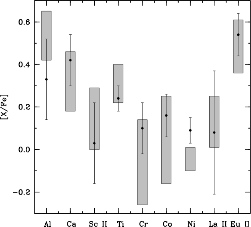
Figure 2: Average abundances for various elements in M10 are shown as filled circles with error bars representing the 1$\sigma$ values. Similar data for M12 from Johnson & Pilachowski (2006) are shown as shaded boxes overlapping the M10 results.

Figure 3: The top panel shows [Al/Fe] versus the horizontal branch parameter, where a value of +1.0 means only BHB stars, 0.0 is a mix of RHB, BHB, and RR Lyrae stars, and –1.0 means only RHB stars. The various symbols indicate the average [Al/Fe] abundance in a cluster with the error bars showing the 1$\sigma$ values. The bottom panel shows [Al/Fe] versus the Galactocentric distance for each cluster. The cluster data are from: M12 (Johnson & Pilachowski 2006), M3 and M13 (Johnson et al. 2005), NGC 7006 (Kraft et al. 1998), M4 (Ivans et al. 1999), M5 (Ivans et al. 2001), and M15 (Sneden et al. 1997).

Table 1: Photometry and Model Atmosphere Parameters

Star	V	B$-$V	Teff	log g	[Fe/H]	vt
			(K)	(cm s-2)	Spectroscopy	(km s-1)
II-85	12.76	1.37	4450	1.20	$-$1.42	1.70
IV-30	12.77	1.44	4450	1.20	$-$1.47	1.90
IV-86	13.13	1.25	4550	1.50	$-$1.42	1.55
III-53	13.80	1.09	4750	1.85	$-$1.44	1.20
IV-49	14.47	1.10	4700	1.85	$-$1.52	1.30

Table 2: Linelist and Equivalent Widths

$\lambda$	Element	E.P.	log gf	III$-$53	III$-$85	IV$-$30	IV$-$49	IV$-$86
(Å)		eV
6696.03	Al I	3.14	$-$1.57	13	12	15	14	26
6698.66	Al I	3.14	$-$1.89	$\cdots$	$\cdots$	$\cdots$	$\cdots$	16
6471.68	Ca I	2.52	$-$0.69	58	112	101	82	98
6499.65	Ca I	2.52	$-$0.82	65	75	108	70	87
6717.68	Ca I	2.71	$-$0.61	$\cdots$	$\cdots$	97	$\cdots$	$\cdots$
6604.60	Sc II	1.36	$-$1.48	26	49	53	40	63
6554.23	Ti I	1.44	$-$1.16	$\cdots$	44	27	22	17
6556.07	Ti I	1.46	$-$1.10	14	30	64	17	38
6743.12	Ti I	0.90	$-$1.65	24	43	48	$\cdots$	42
6559.57	Ti II	2.05	$-$2.30	$\cdots$	55	40	35	45
6606.97	Ti II	2.06	$-$2.79	$\cdots$	22	22	16	14
6630.03	Cr I	1.03	$-$3.49	$\cdots$	$\cdots$	14	$\cdots$	15
6475.63	Fe I	2.56	$-$3.01	44	65	74	36	65
6481.87	Fe I	2.28	$-$3.08	$\cdots$	87	73	$\cdots$	77
6498.95	Fe I	0.96	$-$4.69	$\cdots$	96	90	44	68
6533.93	Fe I	4.56	$-$1.36	14	16	$\cdots$	$\cdots$	15
6546.24	Fe I	2.76	$-$1.54	85	126	$\cdots$	95	107
6574.25	Fe I	0.99	$-$5.02	25	65	69	$\cdots$	45
6592.92	Fe I	2.73	$-$1.47	90	145	132	103	134
6593.88	Fe I	2.43	$-$2.42	65	106	105	$\cdots$	102
6597.57	Fe I	4.79	$-$0.95	$\cdots$	$\cdots$	16	$\cdots$	19
6608.04	Fe I	2.28	$-$3.96	$\cdots$	19	$\cdots$	$\cdots$	26
6609.12	Fe I	2.56	$-$2.69	50	72	103	39	60
6625.02	Fe I	1.01	$-$5.37	$\cdots$	47	37	30	37
6627.54	Fe I	4.55	$-$1.58	$\cdots$	11	$\cdots$	$\cdots$	13
6646.96	Fe I	2.61	$-$3.96	$\cdots$	15	$\cdots$	$\cdots$	$\cdots$
6648.12	Fe I	1.01	$-$5.92	$\cdots$	27	$\cdots$	$\cdots$	15
6677.99	Fe I	2.69	$-$1.35	119	143	160	108	135
6703.57	Fe I	2.76	$-$3.01	25	38	54	$\cdots$	36
6710.32	Fe I	1.48	$-$4.83	$\cdots$	30	44	$\cdots$	31
6726.67	Fe I	4.61	$-$1.07	$\cdots$	$\cdots$	27	14	21
6733.15	Fe I	4.64	-1.48	$\cdots$	11	$\cdots$	$\cdots$	$\cdots$
6739.52	Fe I	1.56	$-$4.79	$\cdots$	$\cdots$	26	$\cdots$	27
6750.16	Fe I	2.42	$-$2.62	53	98	91	69	91
6806.85	Fe I	2.73	$-$3.10	20	38	34	$\cdots$	23
6516.08	Fe II	2.89	$-$3.45	$\cdots$	54	54	35	45
6632.47	Co I	2.28	$-$1.85	9	17	$\cdots$	$\cdots$	18
6482.80	Ni I	1.93	$-$2.79	$\cdots$	74	$\cdots$	40	74
6532.88	Ni I	1.93	$-$3.47	$\cdots$	37	$\cdots$	19	24
6586.31	Ni I	1.95	$-$2.81	31	56	42	$\cdots$	54
6643.63	Ni I	1.68	$-$2.01	98	135	140	84	118
6767.78	Ni I	1.83	$-$2.17	76	102	125	$\cdots$	91
6772.32	Ni I	3.66	$-$0.96	$\cdots$	31	$\cdots$	$\cdots$	27
6774.33	La II	0.13	$-$1.75	$\cdots$	16	29	$\cdots$	7
6645.12	Eu II	1.37	$+$0.20	$\cdots$	24	23	18	22

Table 3: Measured Abundances

Star	[Fe/H]	[Fe II/H]	[Al/Fe]	[Ca/Fe]	[Sc II/Fe]	[Ti/Fe]	[Ti II/Fe]	[Cr/Fe]	[Co/Fe]	[Ni/Fe]	[La II/Fe]	[Eu II/Fe]
III$-$53	$-$1.44	$\cdots$	0.34	0.24	$-$0.20	0.20	$\cdots$	$\cdots$	0.15	0.15	$\cdots$	$\cdots$
III$-$85	$-$1.44	$-$1.40	0.06	0.37	$-$0.10	0.15	0.29	$\cdots$	0.07	0.04	0.04	0.44
IV$-$30	$-$1.49	$-$1.45	0.26	0.49	0.02	0.29	0.20	0.01	$\cdots$	0.01	0.39	0.50
IV$-$49	$-$1.49	$-$1.54	0.43	0.52	0.16	0.31	0.37	$\cdots$	$\cdots$	0.14	$\cdots$	0.67
IV$-$86	$-$1.40	$-$1.43	0.56	0.50	0.29	0.18	0.24	0.19	0.27	0.09	$-$0.18	0.56
Cluster Mean Values
$\langle$$\rangle$	$-$1.45	$-$1.46	0.33	0.42	0.03	0.23	0.28	0.10	0.16	0.09	0.08	0.54
$\sigma$	0.04	0.06	0.19	0.12	0.19	0.07	0.08	0.12	0.10	0.06	0.29	0.10
$\pm$	0.02	0.03	0.08	0.05	0.09	0.03	0.04	0.09	0.06	0.03	0.16	0.05

References

- Andrievsky et al. (2008) Andrievsky, S. M., Spite, M., Korotin, S. A., Spite, F., Bonifacio, P., Cayrel, R., Hill, V., & François, P. 2008, A&A, 481, 481
- Arp (1955) Arp, H. C. 1955, AJ, 60, 317
- Asplund (2005) Asplund, M. 2005, ARA&A, 43, 481
- Busso et al. (1999) Busso, M., Gallino, R., & Wasserburg, G. J. 1999, ARA&A, 37, 239
- Carretta et al. (2007) Carretta, E., Recio-Blanco, A., Gratton, R. G., Piotto, G., & Bragaglia, A. 2007, ApJ, 671, L125
- Carretta (2008) Carretta, E. 2008, Memorie della Societa Astronomica Italiana, 79, 508
- Castelli et al. (1997) Castelli, F., Gratton, R. G., & Kurucz, R. L. 1997, A&A, 318, 841
- Chen et al. (2000) Chen, L., Geffert, M., Wang, J. J., Reif, K., & Braun, J. M. 2000, A&AS, 145, 223
- Cohen & Meléndez (2005) Cohen, J. G., & Meléndez, J. 2005, AJ, 129, 303
- Denissenkov & VandenBerg (2003) Denissenkov, P. A., & VandenBerg, D. A. 2003, ApJ, 593, 509
- Dinescu et al. (1999) Dinescu, D. I., Girard, T. M., & van Altena, W. F. 1999, AJ, 117, 1792
- Fulbright (2000) Fulbright, J. P. 2000, AJ, 120, 1841
- Gehren et al. (2004) Gehren, T., Liang, Y. C., Shi, J. R., Zhang, H. W., & Zhao, G. 2004, A&A, 413, 1045
- Gratton et al. (1999) Gratton, R. G., Carretta, E., Eriksson, K., & Gustafsson, B. 1999, A&A, 350, 955
- Gratton et al. (2004) Gratton, R., Sneden, C., & Carretta, E. 2004, ARA&A, 42, 385
- Iben (1964) Iben, I. J. 1964, ApJ, 140, 1631
- Ivans et al. (1999) Ivans, I. I., Sneden, C., Kraft, R. P., Suntzeff, N. B., Smith, V. V., Langer, G. E., & Fulbright, J. P. 1999, AJ, 118, 1273
- Ivans et al. (2001) Ivans, I. I., Kraft, R. P., Sneden, C., Smith, G. H., Rich, R. M., & Shetrone, M. 2001, AJ, 122, 1438
- Johnson et al. (2005) Johnson, C. I., Kraft, R. P., Pilachowski, C. A., Sneden, C., Ivans, I. I., & Benman, G. 2005, PASP, 117, 1308
- Johnson & Pilachowski (2006) Johnson, C. I., & Pilachowski, C. A. 2006, AJ, 132, 2346
- Kraft (1994) Kraft, R. P. 1994, PASP, 106, 553
- Kraft et al. (1995) Kraft, R. P., Sneden, C., Langer, G. E., Shetrone, M. D., & Bolte, M. 1995, AJ, 109, 2586
- Kraft et al. (1998) Kraft, R. P., Sneden, C., Smith, G. H., Shetrone, M. D., & Fulbright, J. 1998, AJ, 115, 1500
- Kraft & Ivans (2003) Kraft, R. P., & Ivans, I. I. 2003, PASP, 115, 143
- Laird et al. (1988) Laird, J. B., Carney, B. W., Rupen, M. P., & Latham, D. W. 1988, AJ, 96, 1908
- Mishenina et al. (2003) Mishenina, T. V., Panchuk, V. E., & Samus’, N. N. 2003, Astronomy Reports, 47, 248
- Pilachowski et al. (1996) Pilachowski, C. A., Sneden, C., Kraft, R. P., & Langer, G. E. 1996, AJ, 112, 545
- Prochaska & McWilliam (2000) Prochaska, J. X., & McWilliam, A. 2000, ApJ, 537, L57
- Ryan et al. (1996) Ryan, S. G., Norris, J. E., & Beers, T. C. 1996, ApJ, 471, 254
- Smith & Fulbright (1997) Smith, G., & Fulbright, J. 1997, PASP, 109, 1246
- Smith et al. (2005) Smith, G. H., Briley, M. M., & Harbeck, D. 2005, AJ, 129, 1589
- Sneden (1973) Sneden, C. 1973, ApJ, 184, 839
- Sneden et al. (1997) Sneden, C., Kraft, R. P., Shetrone, M. D., Smith, G. H., Langer, G. E., & Prosser, C. F. 1997, AJ, 114, 1964
- Sneden et al. (2004) Sneden, C., Kraft, R. P., Guhathakurta, P., Peterson, R. C., & Fulbright, J. P. 2004, AJ, 127, 2162
- Thévenin & Idiart (1999) Thévenin, F., & Idiart, T. P. 1999, ApJ, 521, 753
- Truran et al. (2002) Truran, J. W., Cowan, J. J., Pilachowski, C. A., & Sneden, C. 2002, PASP, 114, 1293
- von Braun et al. (2002) von Braun, K., Mateo, M., Chiboucas, K., Athey, A., & Hurley-Keller, D. 2002, AJ, 124, 2067
- Woosley & Weaver (1995) Woosley, S. E., & Weaver, T. A. 1995, ApJS, 101, 181
- Yong et al. (2005) Yong, D., Grundahl, F., Nissen, P. E., Jensen, H. R., & Lambert, D. L. 2005, A&A, 438, 875