The Knudsen temperature jump and the Navier-Stokes hydrodynamics of granular gases driven by thermal walls

Abstract

Thermal wall is a convenient idealization of a rapidly vibrating plate used for vibrofluidization of granular materials. The objective of this work is to incorporate the Knudsen temperature jump at thermal wall in the Navier-Stokes hydrodynamic modeling of dilute granular gases of monodisperse particles that collide nearly elastically. The Knudsen temperature jump manifests itself as an additional term, proportional to the temperature gradient, in the boundary condition for the temperature. Up to a numerical pre-factor ${\cal O}(1)$, this term is known from kinetic theory of elastic gases. We determine the previously unknown numerical pre-factor by measuring, in a series of molecular dynamics (MD) simulations, steady-state temperature profiles of a gas of elastically colliding hard disks, confined between two thermal walls kept at different temperatures, and comparing the results with the predictions of a hydrodynamic calculation employing the modified boundary condition. The modified boundary condition is then applied, without any adjustable parameters, to a hydrodynamic calculation of the temperature profile of a gas of inelastic hard disks driven by a thermal wall. We find the hydrodynamic prediction to be in very good agreement with MD simulations of the same system. The results of this work pave the way to a more accurate hydrodynamic modeling of driven granular gases.

I Introduction

Granular gas - a shorthand for a rapid flow of a low-density assembly of inelastically colliding particles - continues to attract much attention gasreviews ; hydrreview ; brilliantov . Not in the least this is because of fascinating pattern-forming instabilities that develop in granular gases: clustering, convection, phase separation, oscillatory instability etc., see e.g. Ref. Aranson for a review. A continuum description of these phenomena is provided by the Navier-Stokes granular hydrodynamics which is derivable, under certain assumptions, from the more basic kinetic theory. For dilute gases this is the Boltzmann equation, properly modified to account for inelastic particle collisions. Within the Chapman-Enskog gradient expansion formalism the above-mentioned assumptions are not specific to granular gases and are the same as in hydrodynamics of elastic hard sphere fluid: (i) the mean free path (and the mean time between two consecutive particle collisions) of the gas should be much smaller than any length scale (correspondingly, time scale) that one attempts to describe hydrodynamically, and (ii) the gas density should be much smaller than the close-packing density of spheres. It is crucial that the validity of these assumptions cannot be guaranteed a priori, as they operate with quantities that become explicitly known only after the hydrodynamic problem in question is solved. Furthermore, as it has been found in numerous recent examples, inelasticity of particle collisions drives strong gradients of hydrodynamic fields. As a result, the scale separation condition [condition (i) above] usually breaks down unless the particle collisions are nearly elastic. The nearly elastic limit is quite restrictive, as it puts a vast majority of granular materials beyond the formal limits of the Navier-Stokes hydrodynamics. Still, this limit proved to be very useful because, with its great predictive power and readily available imagery of macroscopic flow patterns, the Navier-Stokes hydrodynamics gives a valuable insight into complex collective phenomena in granular flows that, at least qualitatively, often persist well beyond the nearly elastic limit.

A direct quantitative measure of scale separation in a gas (both molecular, and granular) is the Knudsen number $K$: the ratio of the (local) mean free path of the gas to a characteristic hydrodynamic length scale. Starting from the Boltzmann equation one obtains, in the zero order approximation in $K\ll 1$, ideal hydrodynamics: the Euler hydrodynamics for the gas of elastically colliding spheres, and the Euler hydrodynamics with bulk energy losses for the granular gas brilliantov ; fouxon1 ; fouxon2 . In the next, first order in $K$ one obtains the Navier-Stokes hydrodynamics Chapman ; LP ; brilliantov . The still higher, second order in $K$ brings two types of new effects: the Burnett correction terms in the hydrodynamic equations and ${\cal O}(K)$ corrections to the boundary conditions Chapman ; LP . The Knudsen numbers of granular flows are typically not very small, therefore the second order effects are often important. It is crucial that, in many cases of interest, the corrections to the boundary conditions are more important than the Burnett correction terms in the hydrodynamic equations. (See, e.g. Ref. LP for a detailed explanation of this fact in the case of molecular gases. This explanation typically holds for dilute granular gases with nearly elastic particle collisions.) The present work deals with a quantitative incorporation of one of the corrections to the boundary conditions - the one corresponding to the Knudsen temperature jump at a thermal wall - in the Navier-Stokes hydrodynamic modeling of dilute granular gases of nearly elastically colliding particles.

The Knudsen temperature jump, and other types of Knudsen jumps/slips of hydrodynamic fields at the system boundaries Chapman ; LP , are intimately related to what is called the Knudsen layer: a next-to-wall region which thickness is comparable to the (local) mean free path of the gas, and where therefore hydrodynamic theory breaks down. Although well known in the context of rarefied molecular gases Chapman ; LP ; Kogan , the physics of the Knudsen layer and its consequences for the bulk flow have received only a cursory attention from the granular community GoldhirschChaos . This is in spite of the fact that the Knudsen numbers of granular flows are typically not small, and temperature jumps were evidently present in, and noticed by the authors of, a number of MD simulations of granular gases driven by thermal walls, see e.g. Refs. Grossman ; Ramirez ; Soto . Furthermore, it was observed Grossman that, inside the Knudsen layer, the particle velocity distribution strongly deviates from a Maxwellian, as the temperature of the particles moving toward the thermal wall is different from that of the outgoing particles.

To our knowledge, the first detailed quantitative study of the role of Knudsen layers in granular gases is the recent work by Galvin et al. Hrenya . They performed three-dimensional MD simulations of a monodisperse granular gas driven by two opposite thermal walls, and compared steady-state hydrodynamic fields, and the steady-state heat flux through the system, with predictions from the Navier-Stokes hydrodynamics with two different sets of constitutive relations accounting for finite-density corrections in the spirit of the Enskog theory. Galvin et al. did not attempt to modify the boundary conditions at the thermal walls. By measuring the deviations between the hydrodynamic theory and simulations, they estimated the effective Knudsen layer thickness as $2.5$ (local) mean free paths. They also observed that Navier-Stokes hydrodynamic calculations that do not account for the presence of Knudsen layers remain accurate “for Knudsen layers collectively composing up to 20% of the domain” Hrenya .

Essentially, the objective of Galvin et al. Hrenya was to establish the validity limits of the Navier-Stokes hydrodynamics that ignores the presence of the Knudsen layers and the corrections to the boundary conditions that appear in the second-order expansion in $K$. The objective of the present work is different: we will take these corrections into account for the purpose of a more accurate description of the hydrodynamic fields in the bulk - outside the Knudsen layers.

The strategy that we suggest makes the full use of a crucial simplification that appears in the limit of nearly elastic particle collisions: the only limit we will focus on. Here the correction term in the boundary condition for the temperature is independent, in the leading order of the theory, of the particle collision inelasticity and can therefore be adopted from the theory of elastically colliding hard sphere fluid. The corrected boundary condition must be satisfied by the hydrodynamic fields extrapolated to the boundary from the bulk, rather than by the true local values of the fields at the boundary; see Ref. LP for a pedagogical review of this important circumstance. Furthermore, up to a single numerical pre-factor, this term is known from kinetic theory Chapman ; LP . We will not attempt to find this pre-factor by solving the Boltzmann equation inside the Knudsen layer (such a solution would be quite involved) and matching the “inner” kinetic solution next to the boundary with the “outer” hydrodynamic solution in the bulk. Instead, we will extrapolate the steady-state temperature profiles in the bulk, measured in MD simulations, to the boundaries. As will be shown shortly, a comparison of the extrapolated values of the gas temperature with those predicted from the hydrodynamics which employs the modified boundary condition yields an estimate of the unknown numerical pre-factor: the only adjustable parameter of our theory. Once the pre-factor is found, the modified boundary condition (with no adjustable parameters) can be used for, and render a more accurate hydrodynamic description of, a host of two-dimensional gases (of either elastic, or weakly inelastic particles, with and without gravity) driven by thermal walls of the same type.

The remainder of the paper is organized as follows. We start Section II with Navier-Stokes hydrodynamic calculations of a steady-state temperature profile of a two-dimensional gas of monodisperse elastic hard disks, confined between two thermal walls kept at different temperatures. The same Section II reports a series of MD simulations of the same system. A comparison between the two yields the unknown numerical pre-factor of the correction term of the modified boundary condition. The modified boundary condition is then applied in Section III to a gas of inelastic hard disks driven by a single thermal wall, and the results are compared with those of MD simulations of the same system. Section IV presents a brief discussion of our results and of related open questions.

II Knudsen temperature jump and modified boundary conditions

Consider a dilute assembly of elastically colliding monodisperse hard disks in a two-dimensional box, confined between two thermal walls located at $x=-L_{x}/2$ and $x=L_{x}/2$ and kept at different temperatures $T_{1}$ and $T_{2}<T_{1}$, respectively. What is the steady-state temperature of the gas next to the thermal wall $x=-L_{x}/2$? There are two different groups of particles here: the outgoing particles with temperature $T_{1}$ and the incoming particles with a smaller temperature. Therefore, the overall gas temperature (defined as the average energy of particles) next to the wall $x=-L_{x}/2$ is smaller than $T_{1}$. By the same argument, the gas temperature next to the wall $x=L_{x}/2$ is larger than $T_{2}$. This is the well known Knudsen temperature jump effect. For small Knudsen numbers, $K\ll 1$, the corrected boundary conditions that accommodate the Knudsen temperature jump for the purpose of hydrodynamic calculations in the bulk have the following form Chapman ; LP

$$\left(T-g_{0}\,\lambda\,\frac{\partial T}{\partial x}\right)\Big{|}_{x=-L_{x}/2}\,=T_{1}\,,$$

$$\left(T+g_{0}\,\lambda\,\frac{\partial T}{\partial x}\right)\Big{|}_{x=L_{x}/2}\,=T_{2}\,,$$ (1)

where $\lambda=(2\sqrt{2}\,d\,n)^{-1}$ is the local mean free path, $d$ is the particle diameter, $n$ is the number density of the gas, and $g_{0}={\cal O}(1)$ is a numerical pre-factor that depends on the exact nature of the boundary. In the following we will assume a most commonly used thermal wall protocol and determine the unknown pre-factor from MD simulations. As $dT/dx<0$, conditions (1) imply that $T<T_{1}$ near the wall $x=-L_{x}/2$, and $T>T_{2}$ near the wall $x=L_{x}/2$, as expected.

Now we employ the Navier-Stokes hydrodynamic (or rather hydrostatic) equations to describe the steady state of this system with a zero mean flow:

$$p=const\;\;\;\mbox{and}\;\;\;\mathbf{\nabla}\cdot(\kappa\mathbf{\nabla}T)=0\,,$$ (2)

where $p$ is the gas pressure, and $\kappa$ is the thermal conductivity. To make the formulation closed we need to specify the equation of state $p=p(n,T)$ and an expression for $\kappa$ in terms of $n$ and $T$. For a dilute gas of elastically colliding hard disks of mass $m=1$ and diameter $d$ these are given by the well known relations

$$p=n\,T\;\;\;\mbox{and}\;\;\;\kappa=\kappa_{0}\,\frac{2\,T^{1/2}}{\pi^{1/2}\,d}\,,$$ (3)

where the pre-factor $\kappa_{0}=1.029$ appears Gass in the third Sonine polynomial approximation Burnett ; Liboff . The normalization condition

$$\int_{-L_{x}/2}^{L_{x}/2}dx\int_{-L_{y}/2}^{L_{y}/2}dy\,n(x,y)\,=\,N\,,$$ (4)

fixes the total number of particles $N$. We are looking for a $y$-independent solution, $n=n(x)\,,T=T(x)$, and rescale variables: ${\mathbf{r}}/L_{x}\to\mathbf{r}\,,T/T_{2}\to T\,,n/\bar{n}\to n$, where $\bar{n}=N/(L_{x}L_{y})$ is the average number density of the gas. Equations (2) become

$$P=const\;\;\;\mbox{and}\;\;\;\frac{d}{dx}\left(T^{1/2}\frac{dT}{dx}\right)=0\,,$$ (5)

where $P=p/(\bar{n}\,T_{2})$ is the rescaled pressure. The boundary conditions (1) become

$$\left(T-\frac{g_{0}\,K}{n}\,\frac{dT}{dx}\right)\Big{|}_{x=-1/2}\,=\delta\,,$$

$$\left(T+\frac{g_{0}\,K}{n}\,\frac{dT}{dx}\right)\Big{|}_{x=1/2}\,=1\,,$$ (6)

where $K=L_{y}/(2\sqrt{2}\,N\,d)\ll 1$ is the effective Knudsen number of the system, and $\delta=T_{1}/T_{2}$. The normalization condition (4) becomes

$$\int_{-1/2}^{1/2}n(x)\,dx\,=\,1\,.$$ (7)

Solving the second of Eq. (5), we arrive at the temperature profile

$$T(x)=(A\,x\,+\,B)^{2/3}\,.$$ (8)

Now we treat the ${\cal O}(K)$ terms in Eqs. (6) as small corrections and obtain the constants $A$ and $B$ up to the first order in $K$:

$$A=1-\delta^{3/2}+3\,K\,g_{0}\,(\delta+1)(\delta^{1/2}-1)\,,$$

$$B=\frac{1+\delta^{3/2}}{2}-\frac{3}{2}\,K\,g_{0}\,(\delta-1)(\delta^{1/2}-1)\,.$$ (9)

The predicted effective temperature jumps,

$$\Delta T_{-}=2\,K\,g_{0}\,\delta^{1/2}\,(\delta^{1/2}-1)$$ (10)

at the wall $x=-1/2$, and

$$\Delta T_{+}=2\,K\,g_{0}\,(\delta^{1/2}-1)$$ (11)

at the wall $x=1/2$, are proportional to the yet unknown numerical pre-factor $g_{0}$.

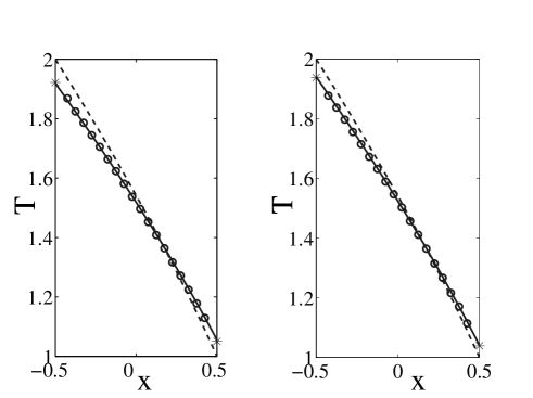
Figure 1: Steady-state temperature versus the rescaled coordinate $x$ for a dilute gas of elastically colliding disks, confined by two thermal walls for $\delta=T_{1}/T_{2}=2$. The circles: MD simulations. The solid lines: predictions from the Navier-Stokes hydrodynamics with the modified boundary conditions Eqs. (8) and (9) with $g_{0}=5.0$. The dashed lines: predictions from the Navier-Stokes hydrodynamics with the boundary conditions $T(x=-1/2)=\delta$ and $T(x=+1/2)=1$ not including the ${\cal O}(K)$ terms. The parameters are $\bar{n}=0.04$, $K=0.01414$, $N=2000$, $L_{x}=625$ and $L_{y}=80$ (the left panel) and $\bar{n}=0.01$, $K=0.01$, $N=16284$, $L_{x}=3540$ and $L_{y}=460$ (the right panel). The wall temperatures, indicated by the asterisks, were determined by linear extrapolation of $T^{3/2}(x)$ from the bulk to the corresponding wall.

To test the hydrodynamic predictions and find the unknown numerical pre-factor $g_{0}$, we performed a series of MD simulations, using an event driven algorithm described in Ref. Rapaport . The walls at $y=\pm L_{y}/2$ were assumed elastic. The thermal walls at $x=\pm L_{x}/2$ were implemented in the simulations in the following way: upon a collision with a thermal wall the normal component of the particle velocity is drawn from a Maxwell distribution with the prescribed wall temperature, while the tangential component of the particle velocity remains unchanged. For each set of parameters we started the simulation from an initially uniform spatial particle distribution and a Maxwell velocity distribution with temperature $T_{2}$, and waited until the gas reached a steady state. This was verified by analyzing the time dependence of the $x$-component of the center of mass of the gas, and the time dependence of the temperature next to the thermal wall at $x=-L_{x}/2$. Then we computed the steady-state temperature profile of the gas by averaging instantaneous temperature profiles over a long time. Figure 1 shows two of the many steady-state temperature profiles measured in our MD simulations. The effective temperature at each of the two walls was obtained by linear extrapolation of the profile of $T^{3/2}(x)$ from the bulk to the wall.

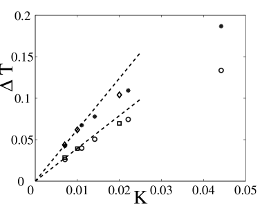
Figure 2: Effective temperature jumps at each of the two thermal walls versus the Knudsen number $K$, as measured in MD simulations (symbols) and predicted by Eqs. (10)-(11) (dashed lines). The lower dashed line, circles and squares correspond to the right wall: $x=1/2$ in the rescaled units. The upper dashed line, diamonds and asterisks correspond to the left wall, $x=-1/2$ in the rescaled units. MD simulations were performed for two different average densities: $\bar{n}=0.04$ (circles and asterisks) and $\bar{n}=0.01$ (squares and diamonds). At $K\lesssim 0.02$ a linear dependence of the effective temperature jumps on $K$ is observed. The linear-dependence part yields $g_{0}=5.0\pm 0.3$. In the simulations with $\bar{n}=0.04$ we varied $K$ by varying the system dimensions $L_{x}$ and $L_{y}$ and keeping a constant total number of particles $N=4000$. In the simulations with $\bar{n}=0.01$, $L_{y}=460$ was kept fixed, while $L_{x}$ and $N$ were varied from $L_{x}=1770$ and $N=8142$, for largest $K$, to $L_{x}=5050$, $N=23230$ for smallest $K$. In all simulations we kept $\delta=T_{1}/T_{2}=2$.

Figure 2 shows the effective temperature jump at each of the two thermal walls as found in our MD simulations at different but small Knudsen numbers and different but small average gas densities. The results for different densities practically coincide. The same figure shows the hydrodynamic predictions from Eqs. (10)-(11). One can see that a linear dependence of the effective temperature jumps on $K$ is observed only for quite small Knudsen numbers: $K\lesssim 0.02$. This linear dependence part yields the pre-factor $g_{0}$:

$$g_{0}=5.0\pm 0.3\,.$$ (12)

Examples of the resulting hydrodynamic temperature profiles, see Eqs. (8) and (9), are depicted in Figure 1, and very good agreement with the MD simulations is observed. The same figure also shows the hydrodynamic temperature profiles calculated with the boundary conditions $T(x=-1/2)=\delta$ and $T(x=+1/2)=1$ not including the ${\cal O}(K)$ terms. As expected, they show a worse agreement with the MD simulations.

In the next section we apply the modified boundary condition with the same value of $g_{0}$ to a granular gas driven by a thermal wall of the same type.

III Granular gas driven by a thermal wall

Having determined the pre-factor $g_{0}$, we can now use the modified boundary condition with this $g_{0}$ for a more accurate hydrodynamic description of two-dimensional gases (of either elastic, or weakly inelastic particles, with and without gravity) driven by thermal wall(s) of the same type. As an example, we will consider here a simple, indeed prototypical, setting: a granular gas confined in a two-dimensional box and driven by a single thermal wall at zero gravity. In a steady state, the energy supplied into this gas from the thermal wall is balanced by the collisional energy loss. The simplest steady state of this system is the so called “stripe state”, where the gas density and temperature fields do not depend on the coordinate parallel to the thermal wall. We will consider the region of parameter where this simple steady state is hydrodynamically stable, see Refs. LMS ; KM for detail.

Let us complete the specification of the model. We consider a dilute assembly of inelastically colliding hard disks of diameter $d$ and mass $m=1$, moving in a box with dimensions $L_{x}\times L_{y}$ at zero gravity. Collisions of disks with the walls $x=0$ and $y=\pm L_{y}/2$ are assumed elastic. The thermal wall, kept at $T=T_{0}$, is located at $x=L_{x}$. The inelasticity of the particle collisions is parameterized by a constant coefficient of normal restitution $r$; we assume the nearly elastic limit $1-r^{2}\ll 1$.

Due to the inelastic particle collisions, the granular temperature decreases with an increase of the distance from the thermal wall. To maintain a constant pressure in a steady state, the particle density must increase with this distance, reaching its maximum value next to the opposite (elastic) wall. The steady state density and temperature profiles of the stripe state are described by the following hydrodynamic/hydrostatic equations [compare with Eqs. (5)]:

$$p=const\;\;\;\mbox{and}\;\;\;\frac{d}{dx}\left(\kappa\frac{dT}{dx}\right)=I\,.$$ (13)

For the nearly elastic collisions, the granular pressure $p$ and the thermal conductivity $\kappa$ are still given by Eq. (3), while

$$I=\sqrt{\pi}\,(1-r^{2})dn^{2}\,T^{3/2}\simeq 2\sqrt{\pi}\,(1-r)dn^{2}\,T^{3/2}$$ (14)

is the energy loss rate of the gas due to the particle collisions, see e.g. Ref. brilliantov , in the limit of $1-r\ll 1$.

Let us rescale the $x$-coordinate by $L_{x}$, the number density of the gas by $\bar{n}$, and the gas temperature by $T_{0}$. Introducing a rescaled inverse density $z(x)=\bar{n}/n(x)$ and rescaled pressure $P=p/(\bar{n}T_{0})$, we can rewrite the second equation in Eqs. (13) in the following form

$$(z^{3/2})^{\prime\prime}=3\,\xi^{2}\,z^{-1/2},$$ (15)

where the primes stand for the derivatives with respect to the rescaled coordinate $x$,

$$\xi=\sqrt{\frac{\pi(1-r)}{2\kappa_{0}}}\,\bar{n}\,d\,L_{x}$$ (16)

is a hydrodynamic inelastic loss parameter, and we recall that $\kappa_{0}=1.029$. The inelastic loss parameter $\xi$ defines the characteristic hydrodynamic length scale of the problem $\xi^{-1}$ or, in the dimensional variables, $\xi^{-1}L_{x}$.

One boundary condition for Eq. (15) can be specified at the elastic wall:

$$z^{\prime}(x=0)=0\,.$$ (17)

Conservation of the total number of particles yields the normalization condition

$$\int_{0}^{1}\frac{dx}{z(x)}=1\,.$$ (18)

Finally, the modified boundary condition at the thermal wall $x=1$ is given by

$$Pz\left(1+g_{0}K\frac{dz}{dx}\right)\Big{|}_{x=1}=1\,.$$ (19)

There are two unknowns in this formulation: the rescaled inverse density $z(x)$ and the constant rescaled pressure $P$. The density profile is completely determined by Eq. (15) and conditions (17) and (18), and can be found analytically in terms of $x=x(z)$ KM . The result is:

$$x=\frac{z_{0}}{2\xi}\left[\mbox{arccosh}\sqrt{\frac{z}{z_{0}}}+\sqrt{\left(\frac{z}{z_{0}}\right)^{2}-\frac{z}{z_{0}}}\right]\,,$$ (20)

where

$$z_{0}=\frac{2\xi}{\xi+\sinh(\xi)\cosh(\xi)}\,.$$

Note that $z(x=1)=z_{0}\cosh^{2}(\xi)$.

In contrast to the density profile, which is independent of the boundary condition (19), the temperature profile is sensitive to the ${\cal O}(K)$ correction in Eq. (19). Using Eq. (19), we calculate the pressure up to the first order in $K$, so that the resulting temperature profile $T(x)=Pz(x)$ is

$$T(x)=\frac{1-2g_{0}K\xi\tanh(\xi)}{z_{0}\cosh^{2}(\xi)}z(x).$$ (21)

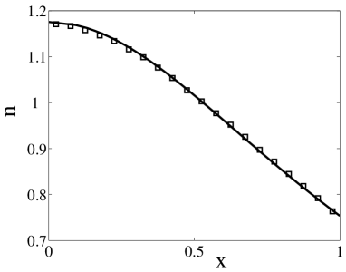
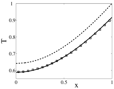
Figure 3: Density (the upper panel) and temperature (the lower panel) profiles of a gas of inelastic hard disks driven by a thermal wall. The theoretical profiles (solid curves) are in good agreement with MD simulations (squares). Shown by the dashed line is the temperature profile obtained without the Knudsen correction. The parameters $N=3540$, $L_{x}=1770$, $L_{y}=200$, and $r=0.999$ correspond to $\xi=0.6916$, $K=0.02$, and $\bar{n}=0.01$.

The hydrodynamic density profile $n(x)=1/z(x)$, given by Eq. (20), and temperature profile, given by Eq. (21), are shown in Fig. 3 (the solid lines in the upper and lower panels, respectively). To test the hydrodynamic results, we performed event-driven MD simulations Rapaport and measured the density and temperature in this system. As before, we verified that the system was in the steady state and computed the profiles, performing averaging over a long time. Figure 3 shows (by the squares) the density (the upper panel) and temperature (the lower panel) as observed in MD simulations. In both cases there is a good agreement between the theoretical profiles and those observed in MD simulations. For comparison, the dashed line in the lower panel of Fig. 3 shows the hydrodynamic temperature profile obtained when ignoring the Knudsen correction in the boundary condition (19). The observed disagreement with the results of MD simulations clearly shows the importance of the Knudsen correction in this example.

Once the hydrodynamic problem is solved, we should verify the scale separation (and the validity of the Navier-Stokes hydrodynamics) by demanding that the mean free path of the gas $\sim(d\bar{n})^{-1}$ be much smaller than the hydrodynamic length scale $\sim L_{x}/\xi\sim(\sqrt{1-r}\,d\bar{n})^{-1}$. This yields a restrictive condition $\sqrt{1-r}\ll 1$ (first obtained in Ref. Grossman ), thus justifying a posteriori our focus on the nearly elastic case.

IV Summary and discussion

We have incorporated the Knudsen temperature jump at thermal wall in the Navier-Stokes hydrodynamic description of weakly inelastic dilute gases of smooth hard disks. We have shown that this procedure may considerably improve the accuracy of hydrodynamic calculations. Therefore, the results of this work pave the way to a more accurate hydrodynamic modeling of driven granular gases. This is important in view of the continuing tests (and the ongoing debate on the validity range) of the Navier-Stokes granular hydrodynamics as a quantitatively accurate theory.

In the prototypical example of a granular gas heated by a thermal wall at zero gravity, that we have considered in this work, the modification of the boundary condition affects only the gas temperature in the bulk, and does not affect the density profile. In more general settings (such as those including gravity), the density profile will be affected as well.

Future work should attempt to extend our approach to other types of Knudsen jumps/slips at the boundaries of rapid granular flows, again in analogy to what has been done in this context for molecular fluids Chapman ; LP . Future work also needs to go beyond the dilute limit and account for finite-density corrections. A practical approach here would be to use the Carnahan-Starling equation of state Carnahan and Enskog-type transport coefficients Jenkins , but still assume nearly elastic collisions. The finite-density case in two dimensions may present difficulties because of the long-lived large-scale hydrodynamic fluctuations which contribute to the transport in addition to the “usual” gradient contributions cohen . These additional contributions formally appear as divergences of the transport coefficients with the system size. Indeed, we observed a clear signature of the apparent divergence of the heat conductivity in our MD simulations when attempting to extend the Knudsen correction to the boundary condition to a moderately dense granular gas in two dimensions. In three dimensions, however, such an extension looks promising.

- (1) Granular Gases, edited by T. Pöschel and S. Luding (Springer, Berlin, 2001); Granular Gas Dynamics, edited by T. Pöschel and N. Brilliantov (Springer, Berlin, 2003).
- (2) I. Goldhirsch, Annu. Rev. Fluid Mech. 35, 267 (2003).
- (3) N.V. Brilliantov and T. Pöschel, Kinetic Theory of Granular Gases, (Oxford University Press, Oxford, 2004).
- (4) I. S. Aranson and L. S. Tsimring, Rev. Mod. Phys. 78, 641 (2006).
- (5) I. Fouxon, B. Meerson, M. Assaf, and E. Livne, Phys. Rev. E 75, 050301(R) 2007; Phys. Fluids 19, 093303 (2007).
- (6) A. Puglisi, M. Assaf, I. Fouxon, and B. Meerson, Phys. Rev. E 77, 021305 (2008).
- (7) S. Chapman and T.G. Cowling, The Mathematical Theory of Non-Uniform Gases (Cambridge Univ. Press, Cambridge, 1990).
- (8) E.M. Lifshitz and L.P. Pitaevskii, Physical Kinetics (Pergamon Press, Oxford, 1981).
- (9) M.N. Kogan, Rarefied Gas Dynamics, (Plenum Press, New York, 1969).
- (10) I. Goldhirsch, Chaos 9, 659 (1999).
- (11) E.L. Grossman, T. Zhou, and E. Ben-Naim, Phys. Rev. E 55, 4200 (1997).
- (12) R. Ramírez, D. Risso, R. Soto, and P. Cordero, Phys. Rev. E 62, 2521 (2000).
- (13) R. Soto, M. Argentina, and M. Clerc, in Granular Gas Dynamics, edited by T. Pöschel and N. Brilliantov (Springer, Berlin, 2003), p. 317.
- (14) J. E. Galvin, C. M. Hrenya, and R. D. Wildman, J. Fluid Mech. 585, 73 (2007).
- (15) D.M. Gass, J. Chem. Phys. 54, 1898 (1971).
- (16) R.L. Liboff, Kinetic Theory: Classical, Quantum, and Relativistic Descriptions (Springer-Verlag, New York, 1998).
- (17) D. Burnett, Proc. London Math. Soc. Ser. 2 39, 385 (1935); 40, 382 (1935).
- (18) D.C. Rapaport, The Art of Molecular Dynamics Simulation Cambridge University Press, Cambridge, 1995.
- (19) E. Livne, B. Meerson, and P.V. Sasorov, Phys. Rev. E 65, 021302 (2002).
- (20) E. Khain and B. Meerson, Phys. Rev. E 66, 021306 (2002).
- (21) N. F. Carnahan and K. E. Starling, J. Chem. Phys. 51, 635 (1969).
- (22) J. T. Jenkins and M. W. Richman, Arch. Ration. Mech. Anal. 87, 355 (1985).
- (23) E.G.D. Cohen, Physica A 194, 229 (1993).