The Schrödinger equation with piercings

Abstract

We show that the spectrum of the Schrödinger equation in two or higher dimensions does not change when Dirichlet boundary conditions are enforced on a number of isolated points inside the original domain (piercings). We have obtained the analytical solution for spherically symmetric state of the $d$-dimensional simple harmonic oscillator pierced at the origin. Results for the case with multiple piercings are obtained numerically and agree with the theoretical prediction. In the case of a two dimensional parabolic quantum dot with two electrons and a single piercing in the origin we show that the energy of the ground state calculated to first order in perturbation theory goes over to the equivalent result in absence of piercing as the radius of the piercing becomes infinitesimal. Interestingly, we find that the leading finite size correction to the interaction energy is negative while the corresponding correction to the single particle energies is (as expected) positive. For a finite radius of the piercing and above a critical coupling, the first term dominates the second and the total energy of the dot with piercing is lower. Unfortunately the critical coupling found for this example is nonperturbative. Finally we study configurations allowing bound states in the continuum, showing that bound states survive to the insertion of piercings and that their energy is unchanged when the radius of the piercing vanishes.

I Introduction

It is a well known result that the frequencies of a membrane do not change when Dirichlet boundary conditions are enforced on a number of isolated points inside the domain of the membrane: this curious result, which at first seems to be at odds with common sense, was first conjectured by Lord Rayleigh long time ago Ray . More recently this problem has received attention in a number of papers, see for example Wang98 ; Gottlieb99 ; Laura99 ; Laura99b ; Wang00 ; Wang01 ; Wang_Yu_01 . In particular, in ref. Wang01 Wang has obtained a general expression for the correction to the frequencies of a membrane with $N$ internal circular regions of infinitesimal radius where no vibration occurrs: these corrections are seen to decay proportionally to $1/\log r_{0}$, $r_{0}$ being the radius of the circular cores. In the present paper we show that these interesting results can be extended to Quantum Mechanics, at least for non–interacting particles. In Section II we derive a general formula for the correction to the energies of the Schrödinger equation in any number of dimensions, $d\geq 2$, with $N$ internal points of infinitesimal radius, where Dirichlet boundary conditions are enforced (we will refer to these points as to ”piercings” throught all the paper). The case $d=2$ confirms the logarithmic behaviour of the corrections already observed in the classical membrane vibration countepart, while a power-like behaviour is found for higher dimensions. In Section III we use the simple harmonic oscillator with a single piercing in the origin (pSHO) as the natural testing ground of the general results obtained: in this case we are able to confirm analytically the predictions of Section II. The case with multiple piercings, on the other hand, is studied numerically, leading to a further confirmation of the results. An interesting question that may be asked is whether the same conclusions of Sections II and III can be reached for $N$ interacting quantum particles in $d$ dimensions: since the problem is clearly too difficult to be attacked on general grounds, we have restricted our attention to a two dimensional parabolic quantum dot, with two electrons, which has been studied in ref. Cifja04 . In this case we have been able to show that, to first order in perturbation theory, the energy of the $2D$ quantum dot with a piercing in the origin is unchanged for $r_{0}\rightarrow 0$; on the other hand we have obtained that the leading order finite size correction to the energy is not definite positive and indeed may become negative if the coupling of the Coulomb interaction is strong enough. Although the critical coupling where the change in sign occurrs is too large to trust a first order perturbative calculation, we believe that this result opens the question on whether the energy of the ground state of a quantum dot could be lowered adding one or more piercings of small but finite size. In Section V we have applied our results to the study of open systems supporting a bound state Exner89 ; Schult89 ; Avishai91 ; Jaffe92 ; Trefethen06 , obtaining numerical results for the crossed wire configuration of Ref.Schult89 which confirm our predictions. In this way we prove that these bound states survive to the inclusion of piercings, even for piercings of finite extension. Finally, Section VI contains our conclusions.

II General considerations

Consider the stationary Schrödinger equation (SSE) in $d$ spatial dimensions

$$-\frac{\hbar^{2}}{2m}\nabla^{2}_{d}\psi(x_{1},\dots,x_{d})+V(x_{1},\dots,x_{d})\psi(x_{1},\dots,x_{d})=E\psi(x_{1},\dots,x_{d})$$ (1)

where $(x,y)\in{\cal D}$ and Dirichlet boundary conditions are enforced on $\partial{\cal D}$. Let $P_{i}=(x_{1}^{(i)},\dots,x_{d}^{(i)})$ be a point internal to ${\cal D}$, where Dirichlet b.c. are also imposed. The index $i$ ranges from $1$ to $N$, i.e. the total number of internal points with Dirichlet bc. We call $\partial{\cal D}^{*}=\partial{\cal D}\ \cup\ \sum_{i=1}^{N}P_{i}$. In this case the SSE reads

$$-\frac{\hbar^{2}}{2m}\nabla^{2}_{d}\phi(x_{1},\dots,x_{d})+V(x_{1},\dots,x_{d})\phi(x_{1},\dots,x_{d})=E^{\prime}\phi(x_{1},\dots,x_{d})\ ,$$ (2)

$E^{\prime}$ and $\phi$ being the new eigenvalue and wave function respectively. Assuming that $V(x_{1},\dots,x_{d})$ is real and using the two equations we can write

$$(E-E^{\prime})\phi^{*}\psi = -\frac{\hbar^{2}}{2m}\left[\phi^{*}\nabla^{2}_{d}\psi-\psi\nabla^{2}_{d}\phi^{*}\right]=\vec{\nabla}\cdot\vec{J}\ ,$$ (3)

where

$$\vec{J}\equiv-\frac{\hbar^{2}}{2m}\left[\phi^{*}\vec{\nabla}_{d}\psi-\psi\vec{\nabla}_{d}\phi^{*}\right]\ .$$ (4)

After integrating eq. (3) over $\cal D$ one has

$$E^{\prime}=E-\frac{\int_{{\cal D}}\vec{\nabla}\cdot\vec{J}d^{d}x}{\int_{{\cal D}}\phi^{*}(x,y)\psi(x,y)d^{d}x}\ .$$ (5)

We use Gauss theorem to convert the integral over the $d$-dimensional volume of ${\cal D}$ in the numerator into an integral over $\partial{\cal D}^{*}$:

$$\int_{{\cal D}}\vec{\nabla}\cdot\vec{J}d^{d}x=\int_{\partial{\cal D}}\vec{J}\cdot d\vec{S}_{d-1}+\sum_{i=1}^{N}\int_{P_{i}}\vec{J}\cdot d\vec{S}^{(i)}_{d-1}\ ,$$ (6)

where $S_{d-1}$ is the surface of ${\cal D}$ and $S_{d-1}^{(i)}$ is the surface of a $d$-sphere centered in $P_{i}$ with infinitesimal radius. Since both $\psi$ and $\phi$ obey Dirichlet bc on $\partial{\cal D}$, the first integral vanishes.

On an $d-1$ sphere of infinitesimal radius $r_{0}$ around the point $P_{i}$ where Dirichlet boundary conditions are imposed one can express locally the solution, $\phi$, as a linear combination of the regular solution $\psi$ and of a solution $\xi$ which diverges at $P_{i}$:

$$\phi\approx\psi+v_{d}\xi$$ (7)

where $v_{d}$ is a constant to be determined by the condition $\phi(r_{0})=0$.

Keeping only the laplacian term in the Schroedinger equation, we approximate $\xi$ with the solution of the $d$-dimensional Poisson equation, diverging at $P_{i}$:

$$\xi(r)=\left\{\begin{array}[]{cc}\log r&d=2\\ \frac{1}{r^{d-2}}&d>2\end{array}\right.$$ (10)

We therefore obtain

$$v_{d}(r_{0})=\left\{\begin{array}[]{cc}-\frac{\psi(r_{0})}{\log r_{0}}&d=2\\ -\psi(r_{0})r_{0}^{d-2}&d>2\end{array}\right.$$ (13)

After taking into account these observations, and neglecting the terms which vanish after integration we have

$$\int_{{\cal D}}\vec{\nabla}\cdot\vec{J}d^{d}x = \sum_{i=1}^{N}\frac{\hbar^{2}}{2m}v_{d}^{(i)}\psi(r_{0}^{(i)})\int_{P_{i}}\vec{\nabla}\xi^{*}\cdot d\vec{S}^{(i)}_{d-1}=-\sum_{i=1}^{N}\frac{\hbar^{2}}{2m}v_{d}^{(i)}\psi(r_{0}^{(i)})\vec{\nabla}\xi^{*}\cdot\hat{r}|_{r_{0}^{(i)}}S^{(i)}_{d-1}\ ,$$ (14)

where $S^{(i)}_{d-1}$ is the surface of a $d-1$ sphere, which is given by

$$S^{(i)}_{d-1}=\frac{2\pi^{d/2}r_{0}^{d-1}}{\Gamma(d/2)}\ .$$ (15)

Therefore we may write:

$$\int_{{\cal D}}\vec{\nabla}\cdot\vec{J}d^{d}x = \left\{\begin{array}[]{cc}\sum_{i=1}^{N}\frac{\hbar^{2}\pi}{m}\frac{\psi^{2}(r_{0}^{(i)})}{\log r_{0}^{(i)}}&d=2\\ \sum_{i=1}^{N}\frac{\hbar^{2}}{m}\psi^{2}(r_{0}^{(i)})(d-2)(r_{0}^{(i)})^{d-2}\frac{\pi^{d/2}}{\Gamma(d/2)}&d>2\end{array}\right.$$ (18)

Let us now come to the denominator in eq. (5): since we expect that the wave function in the presence of piercing be sensibly modified only in the close neighborhood of the points themselves, and the wave functions being normalized, we may argue that $\int_{{\cal D}}\phi^{*}(x,y)\psi(x,y)d^{d}x\approx 1$. The leading behaviour of the energy for $r_{0}\rightarrow 0$ can thus be obtained from eq. (18).

An alternative –qualitative – argument to convince the reader of the isospectrality could be the following: consider the wave function

$$\phi(x_{1},\dots,x_{d})=\psi(x_{1},\dots,x_{d})\ \Xi(x_{1},\dots,x_{d})$$ (19)

where

$$\Xi(x_{1},\dots,x_{d})\equiv\prod_{i=1}^{N}\xi^{(i)}(x_{1},\dots,x_{d})$$ (20)

and $\xi^{(i)}$ is the solution to the homogeneous Poisson equation singular at a point $P_{i}$ internal to ${\cal D}$ and vanishing on an infinitesimal circle of radius $r_{0}$. $\psi(x_{1},\dots,x_{d})$ is the solution in absence of piercing. We substitute $\phi$ in eq. (2) and we obtain the equation:

$$-\frac{\hbar^{2}}{2m}\ \left[2\vec{\nabla}\psi\cdot\vec{\nabla}\Xi+\psi\nabla^{2}\Xi\right]+(E-E^{\prime})\phi(x_{1},\dots,x_{d})=0\ .$$ (21)

If we multiply this equation by $\phi$ and integrate over the $d$ dimensional volume we have

$$(E-E^{\prime})=\frac{\hbar^{2}}{2m}\ \int_{{\cal D}^{*}}\phi\left[2\vec{\nabla}\psi\cdot\vec{\nabla}\Xi+\psi\nabla^{2}\Xi\right]d^{d}x\ .$$ (22)

Since the expression in the square brackets is a function which is singular at all the internal points $P_{i}$, we expect that the main contribution to the integral comes from these regions. Around these points, however, $\phi=0$, and therefore we may expect that

$$\Delta E=\int_{{\cal D}^{*}}\phi\left[2\vec{\nabla}\psi\cdot\vec{\nabla}\Xi+\psi\nabla^{2}\Xi\right]d^{d}x\approx 0\ ,$$ (23)

implying that $E^{\prime}\approx E$.

We can also provide a more direct proof of this statement by considering the special case of a single piercing in two dimensions, which can then be generalized to $N$ piercings in $d$ dimensions. In this case eq. (19) reads

$$\phi(x,y)=\psi(x,y)\ \log\frac{r}{r_{0}}\ .$$ (24)

As it stands this expression is not normalized and we should rather write

$$\tilde{\phi}(x,y)=\frac{\psi(x,y)\ \log\frac{r}{r_{0}}}{\sqrt{\int_{{\cal D}^{*}}|\psi(x,y)|^{2}\log^{2}\frac{r}{r_{0}}dxdy}}\ .$$ (25)

If we now take the limit $r_{0}\rightarrow\infty$,for $r>r_{0}$, we have

$$\lim_{r\rightarrow r_{0}}\tilde{\phi}(x,y)=\psi(x,y)$$ (26)

which supports the conclusions previously reached.

Since the results obtained in this Section concern the inclusion of isolated Dirichlet points in the $d$ dimensional domain where the SSE is defined, the reader may wonder at this point if it is possible to find regions of dimension $0<d^{\prime}<d-2$ which leave the spectrum invariant when Dirichlet bc are enforced. In this case the application of Gauss theorem must be specific to the problem, since $S_{d-1}^{(i)}$ will be now the infinitesimal surface enclosing the Dirichlet region. We may however convince ourselves that it is indeed possible by looking at a specific example: consider the Hamiltonian for a $d\geq 3$ problem, which is separable in the form $\hat{H}=\hat{H}_{1\dots k}+\hat{H}_{k+1,\dots,d}$, where $k\geq 2$. Here $\hat{H}_{1\dots k}$ contains the coordinates $x_{1},\dots,x_{k}$ and their conjugate momenta, while $\hat{H}_{k+1,\dots,d}$ contains the remaining coordinates and momenta. In this case the solution of the problem is obtained as the direct product of the solutions of $\hat{H}_{1\dots k}$ and $\hat{H}_{k+1,\dots,d}$ respectively. Therefore, adding $N$ piercings of infinitesimal size to $\hat{H}_{1\dots k}$ can be interpreted as adding $N$ regions of dimension $d-k$ with Dirichlet boundary conditions to the original domain. Since the spectrum of $\hat{H}_{1\dots k}$ is unchanged under this operation, we conclude that the same is true for the total hamiltonian $\hat{H}$.

III The simple harmonic oscillator in $d$ dimensions pierced in the origin

The simple harmonic oscillator in $d>2$ dimensions is the ideal test of the results presented in the previous section, given that analytical results can be obtained. The SSE in this case reads

$$\left[-\frac{\hbar^{2}}{2\mu}\nabla_{d}^{2}+\frac{1}{2}\mu\omega^{2}(x_{1}^{2}+\dots+x_{d}^{2})-E\right]\psi(x_{1},\dots,x_{d})=0\ ,$$

where $\nabla_{d}^{2}$ is the Laplacian operator in $d$ dimensions. For simplicity we study only spherically symmetric states with zero angular momentum and therefore consider only the radial part of the Laplacian ($\nabla_{d}^{2}\rightarrow\frac{\partial^{2}}{\partial r^{2}}+\frac{d-1}{r}\frac{\partial}{\partial r}$). 

After introducing the standard dimensionless variables $\rho\equiv\sqrt{\mu\omega/\hbar}\ r$ and $\epsilon\equiv E/\hbar\omega$  we write $\psi(\rho)=e^{-\rho^{2}/2}\xi(\rho)$ and obtain the differential equation

$$\xi^{\prime\prime}(\rho)+\left(\frac{d-1}{\rho}-2\rho\right)\xi^{\prime}(\rho)+\left(2\epsilon-d\right)\xi(\rho)=0\ .$$ (27)

We wish to solve this equation subject to the conditions $\xi(\rho_{0})=0$ and $\lim_{\rho\rightarrow\infty}\psi(\rho)=0$, so that the wave function be square integrable on the domain. After enforcing the first condition we obtain the solution:

$$\xi(\rho) = \left[U\left(\frac{d-2\epsilon}{4},\frac{d}{2},\rho_{0}^{2}\right)L_{\frac{\epsilon}{2}-\frac{d}{4}}^{\frac{d}{2}-1}\left(\rho^{2}\right)-U\left(\frac{d-2\epsilon}{4},\frac{d}{2},\rho^{2}\right)L_{\frac{\epsilon}{2}-\frac{d}{4}}^{\frac{d}{2}-1}\left(\rho_{0}^{2}\right)\right]$$

where $U$ and $L$ are the hypergeometric $U$ and the Laguerre $L$ functions. Since the Laguerre function blows up at infinity the full solution also blows up unless the condition

$$U\left(\frac{d-2\epsilon}{4},\frac{d}{2},\rho_{0}^{2}\right)=0$$ (29)

is met. As we see in Fig. 1, which displays $\Omega(\epsilon,\rho_{0})\equiv\frac{U\left(\frac{2-2\epsilon}{4},1,\rho_{0}^{2}\right)}{\log_{10}1/\rho_{0}\ \sqrt{\epsilon}\ \Gamma\left(\frac{\epsilon}{2}\right)}$ for $\rho_{0}=10^{-3}$, the zeroes of this function are slightly displaced to the right with respect to the unperturbed values, represented with circles. Notice that for specific values of the energy, the expression for the wave function simplify: for example, in two dimensions, for $\epsilon=2k+1$, with $k$ integer, one goes over to the wave functions of the excited states of the unpierced oscillator (this corresponds to setting $\rho_{0}$ in the largest positive node of such wave function). For $\epsilon=3$ one has $\xi(\rho)\propto(1-\rho^{2})$, corresponding to $\rho_{0}=1$; for $\epsilon=5$, one has $\xi(\rho)\propto(2-4\rho^{2}+\rho^{4})$, corresponding to $\rho_{0}=\sqrt{2+\sqrt{2}}$.

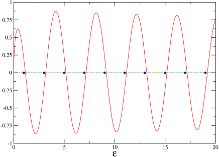
Figure 1: $\Omega(\epsilon,\rho_{0})\equiv\frac{U\left(\frac{2-2\epsilon}{4},1,\rho_{0}^{2}\right)}{\log_{10}1/\rho_{0}\ \sqrt{\epsilon}\ \Gamma\left(\frac{\epsilon}{2}\right)}$ for $\rho_{0}=10^{-3}$ as a function of $\epsilon$. (color online)

In particular we are interested in knowing the behaviour of the energies of the ground state for $\rho_{0}\rightarrow 0$: for $d=2$ we obtain that $\epsilon^{(2)}\approx 1-1/\log\rho_{0}$, whereas for $d>2$ we have $\epsilon^{(d)}\approx d/2+c^{(d)}\ \rho_{0}^{d-2}$, where $c^{(d)}=2/\Gamma(d/2-1)$. Notice that this expression for $c^{(d)}$ coincides with the general expression in eq. (18).

We can now use eq. (LABEL:exact0) to extract the dominant behaviour of the exact solution as $\rho_{0}\rightarrow 0$. In the limit $r\rightarrow 0$, for the ground state, the confluent hypergeometric function behaves as

$$U(a,\frac{d}{2},r^{2})\approx\left\{\begin{array}[]{cc}-2a\log r&d=2\\ a\frac{\Gamma(d/2-1)}{r^{d-2}}&d>2\end{array}\right.$$ (32)

which confirms eq. (19).

In the left plot of Fig.2 we display the quantity $\Xi(r_{0})\equiv(\epsilon_{d}-d/2)/r_{0}^{d-2}$ for the ground state of the SHO pierced in the origin in $d=2,3,4,5$ dimensions for small values of $r_{0}$. The horizontal lines are the coefficients $c_{d}$ obtained directly from the exact solution and from the general formula, given in the previous section. In the right plot of Fig.2 we compare the exact solution of eq. (LABEL:exact0) and the asymptotic one of eq. (19), both corresponding to a piercing radius $r_{0}=10^{-10}$, with the solution for the oscillator without piercing.

The energy of the ground state of the pierced sho can be estimated precisely even in the case where the radius of the pierced region is sizeable using a variational approach. In this case we use a trial wave function

$$\psi(\rho)=N\ e^{-\rho^{2}/2}\ \log\left(\frac{\rho}{\rho_{0}}\right)\ \left(1+a\rho^{b}\right)$$ (33)

for $d=2$ and

$$\psi(\rho)=N\ e^{-\rho^{2}/2}\ \left(\frac{1}{\rho^{d-2}}-\frac{1}{\rho_{0}^{d-2}}\right)\ \left(1+a\rho^{b}\right)$$ (34)

for $d>2$. Here $N$ is a normalization constant and $a$ and $b$ are variational parameters. In the left part of Fig. 3 we show the energy of the ground state of the pierced sho, as a function of the pinning radius, $r_{0}$, for $d=2,3,4,5$. In the limit $r_{0}\rightarrow 0$ the energies tend to the energy of the unpierced sho, whereas for $r_{0}>1$ the curves approach a universal behaviour, which is dominated by the potential energy. Notice that the symbols correspond to the energy calculated numerically using the exact expression, while the lines correspond to the variational results.

We briefly address the problem of a SHO with $N$ piercings in two dimensions. Although this problem cannot be solved exactly for an arbitrary radius of the piercing, its spectrum should still go over to the unperturbed spectrum as the radius of the piercing goes to zero, with a logarithmic strength which is given by eq. (18). In Table 1 we compare the numerical results for the energy and the leading coefficient $c^{(2)}$, obtained by fitting the energy obtained using the expectation value of the hamiltonian in the asymptotic wave function for $r_{0}$ going from $10^{-30}$ to $10^{-20}$, with the theoretical predictions obtained in Section II. The overlap between the asymptotic and unperturbed wave functions has been calculated numerically for $r_{0}=10^{-50}$: this overlap, as anticipated, is fairly close to $1$ and simply assuming it $1$ would lead to $c^{(2)}=N\ e^{-1/9}\approx 0.894839N$.

The right plot of Fig. 3 displays the energy of the ground state of the SHO with $N$ piercings uniformly distributed on a circle of radius $R=1/3$. The plot of the asymptotic wave function for the SHO with $20$ piercing of radius $r_{0}=10^{-10}$ is shown in Fig.4.

Table 1: Theoretical and numerical results for the energy and the leading coefficient $c^{(2)}$ of a SHO which contains $N$ piercings uniformly distributed on a circle of radius $1/3$.

$N$	$\epsilon_{th}$	$\epsilon_{FIT}$	$c_{th}^{(2)}/N$	$c_{FIT}^{(2)}/N$
2	1	0.9999977	0.8948766	0.8950938
3	1	0.9999314	0.8948683	0.8987901
4	1	0.9999960	0.8949873	0.8950401
10	1	0.9998796	0.8956917	0.8976956
20	1	0.9993188	0.8983882	0.9036415

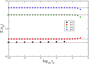
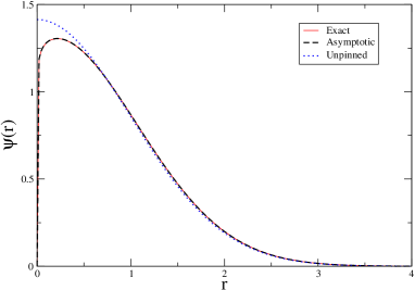
Figure 2: Left plot:$\Xi(r_{0})\equiv(\epsilon_{d}-d/2)/r_{0}^{d-2}$ for the ground state of the simple harmonic oscillator in $d$ dimensions, pierced at the origin. Right plot:Wave function for the ground state of the sho: the solid and dashed lines correspond to the exact and asymptotic solutions for the sho pierced at the origin; the dotted line is the unpierced sho. The parameter $r_{0}=10^{-10}$ is used in the first two curves. (color online)

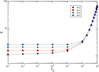
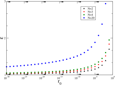
Figure 3: Left plot: Energy of the ground state of the $d$-dimensional simple harmonic oscillator as a function of the radius $r_{0}$ of the internal region where the wave function vanishes. The symbols correspond to the numerical solution of the exact equation, whereas the dashed lines correspond to the variational estimate. Right plot:Energy of the ground state of the two dimensional quantum dot with $N$ piercings uniformly distributed at a distance $d=1/3$ from the origin, calculated using the asymptotic wave function. We use $\hbar=m=\omega=1$ and plot the energy as a function of the radius $r_{0}$. (color online)

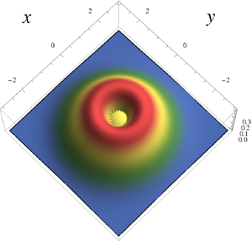
Figure 4: Asymptotic wave function for the SHO pierced on $20$ points uniformly distributed on a circle of radius $R=1/3$. In this case $r_{0}=10^{-10}$. (color online)

IV Ground state of a two dimensional parabolic quantum dot

We now consider a two electron system confined by a 2D parabolic potential in a zero magnetic field. Ref. Cifja04 contains an analytical expression for the first order contribution to the ground state energy of this system in nondegenerate perturbation theory. We will first review the main steps of this calculation for the unpierced quantum dot and then extend the calculation to the quantum dot pierced in the origin.

The hamiltonian for this problem is

$$\hat{H}(\vec{r_{1}},\vec{r_{2}})=\frac{\hat{p}_{1}^{2}}{2\mu}+\frac{\mu\omega^{2}r_{1}^{2}}{2}+\frac{\hat{p}_{2}^{2}}{2\mu}+\frac{\mu\omega^{2}r_{2}^{2}}{2}+\frac{e^{2}}{|\vec{r}_{1}-\vec{r}_{2}|}\ ,$$ (35)

where the last term provides the Coulomb repulsion between the electrons.

In the absence of this term the total wave function is obtained as the direct product of the single particle wave functions of a simple harmonic oscillator, which are given by:

$$\Phi_{n,m}(r,\phi)=N_{nm}\frac{e^{im\phi}}{\sqrt{2\pi}}\ (\alpha r)^{m}\ e^{-\alpha^{2}r^{2}/2}L_{n}^{|m|}(\alpha^{2}r^{2}),$$ (36)

where $L_{n}^{m}$ are the associated Laguerre polynomials. $N_{nm}=\sqrt{2n!\alpha^{2}/(n+|m|)!}$ is the normalization factor and $\alpha\equiv\sqrt{\mu\omega/\hbar}$. The single particle energies are given by

$$E_{nm}=\hbar\omega(2n+|m|+1),$$ (37)

with $n=0,1,\dots$ and $m=0,\pm 1,\pm 2,\dots$. The single particle wave function for the ground state is simply

$$\Phi_{00}(r,\phi)=\frac{\alpha}{\sqrt{\pi}}e^{-\alpha^{2}r^{2}/2}\ .$$ (38)

In the ground state of the two particle system the electrons form a spin singlet and therefore the orbital wave function is symmetric in the electron coordinates:

$$\Psi(\vec{r}_{1},\vec{r}_{2})=\Phi_{00}(\vec{r}_{1})\Phi_{00}(\vec{r}_{2})\ \left[\frac{\chi_{+,1}\chi_{-,2}-\chi_{+,2}\chi_{-,1}}{\sqrt{2}}\right]\ .$$ (39)

Treating the Coulomb repulsion between the electrons as a perturbation, the authors of Ref. Cifja04 have obtained an analytic expression for the first order correction in nondegenerate perturbation theory:

$$\Delta E^{(1)} = \left(\frac{\alpha^{2}}{\pi}\right)^{2}\ \int d^{2}r_{1}\int d^{2}r_{2}e^{-\alpha^{2}(r_{1}^{2}+r_{2}^{2})}\ \frac{e^{2}}{|\vec{r}_{1}-\vec{r}_{2}|}=e^{2}\alpha\sqrt{\frac{\pi}{2}}\ ,$$ (40)

using the identity 

$$\frac{1}{|\vec{r}_{1}-\vec{r}_{2}|}=\sum_{m=-\infty}^{+\infty}\int_{0}^{\infty}dke^{im(\phi_{1}-\phi_{2})}\ J_{m}(kr_{1})\ J_{m}(kr_{2})\ .$$ (41)

We may now discuss the same problem in the presence of a piercing in the origin. As previously found, the single particle wave function for the ground state in presence of piercing of infinitesimal radius $r_{0}$ is simply given by

$$\tilde{\Phi}_{00}(\vec{r})=\tilde{N}_{00}\ e^{-\alpha^{2}r^{2}/2}\ \log\frac{r}{r_{0}}.$$ (42)

The normalization constant is expressed in term of the Meijer $G$ function as

$$\tilde{N}_{00}=\alpha\sqrt{\frac{2}{\pi\ G_{2,3}^{3,0}\left(\alpha^{2}{r_{0}}^{2}\left|\begin{array}[]{c}1,1\\ 0,0,0\end{array}\right.\right)}}\ ,$$ (45)

and $\tilde{N}_{00}\rightarrow-\frac{\alpha}{\sqrt{\pi}\log\alpha r_{0}}+\frac{\alpha\gamma}{2\sqrt{\pi}\log^{2}\alpha r_{0}}$ for $r_{0}\rightarrow 0$.

The perturbative correction to the ground state energy is therefore given by

$$\Delta\tilde{E}^{(1)} = e^{2}\tilde{N}_{00}^{4}\int d^{2}r_{1}\int d^{2}r_{2}\ \log^{2}\frac{r_{1}}{r_{0}}\log^{2}\frac{r_{2}}{r_{0}}\ e^{-\alpha^{2}(r_{1}^{2}+r_{2}^{2})}\ \frac{e^{2}}{|\vec{r}_{1}-\vec{r}_{2}|}$$ (46)

$$= e^{2}\tilde{N}_{00}^{4}\int_{0}^{\infty}dk\left[\int d^{2}r\log^{2}\frac{r}{r_{0}}e^{-\alpha^{2}r^{2}}\ J_{0}(kr)\right]^{2}$$

In order to evaluate the integral in the square bracket we use the series representation

$$J_{0}(z)=\sum_{j=0}^{\infty}\frac{(-1)^{j}}{j!^{2}}\ \left(\frac{z}{2}\right)^{2j}\ ,$$ (47)

and evaluate the integral

$${\cal I}_{j} \equiv \int_{r_{0}}^{\infty}dr\ r^{2j+1}\log^{2}\frac{r}{r_{0}}e^{-\alpha^{2}r^{2}}=\frac{1}{4}\alpha^{-2(j+1)}G_{3,4}^{4,0}\left(\alpha^{2}{r_{0}}^{2}\left|\begin{array}[]{c}1,1,1\\ 0,0,0,j+1\end{array}\right.\right)$$ (50)

$$\approx \frac{j!}{2\alpha^{2(j+1)}}\ \left[\log^{2}(\alpha{r_{0}})-\log(\alpha{r_{0}})\psi^{(0)}(j+1)+\dots\right]$$ (51)

where $\psi^{(0)}(j+1)$ is the polygamma function given by $\psi^{(0)}(z)=\sum_{k=1}^{\infty}\left[\frac{1}{k}-\frac{1}{k+z-1}\right]-\gamma$. We use this expression, together with eq. (47), to write eq. (46) as

$$\Delta\tilde{E}^{(1)} \approx 4\pi^{2}e^{2}\tilde{N}_{00}^{4}\int_{0}^{\infty}dk\frac{1}{4\alpha^{4}}e^{-\frac{k^{2}}{2\alpha^{2}}}\left[\log^{4}\alpha r_{0}-2\left(\Gamma\left(0,-\frac{k^{2}}{4\alpha^{2}}\right)\right.\right.$$ (52)

$$+ \left.\left.\log\left(-\frac{k^{2}}{4\alpha^{2}}\right)\right)^{2}\log^{3}(\alpha{r_{0}})+\dots\right]=e^{2}\alpha\left[\sqrt{\frac{\pi}{2}}+\frac{\kappa-\sqrt{2\pi}\gamma}{\log\alpha r_{0}}+\dots\right]$$

where $\kappa\equiv-2\int_{0}^{\infty}dke^{-\frac{k^{2}}{2}}\left(\Gamma\left(0,-\frac{k^{2}}{4}\right)+\log\left(-\frac{k^{2}}{4}\right)\right)\approx 2.240700135$. This equation tells us that in the limit $r_{0}\rightarrow 0$ the interaction energy to first order in PT is exactly the same as in the case of the quantum dot without piercing, while the leading finite size correction to this energy is negative. In other words, at least to first order in PT, the presence of a piercing lowers the interaction energy. Combining this expression with the leading order expression for the single particle energy we obtain the total energy to first order in PT goes as

$$E_{TOT}\approx\hbar\omega\left\{2+\lambda\sqrt{\frac{\pi}{2}}-\frac{1}{\log\alpha r_{0}}\left[2-(\kappa-\sqrt{2\pi}\gamma)\lambda\right]\right\}$$ (53)

where $\lambda\equiv\frac{e^{2}\alpha}{\hbar\omega}$, using the notation of Ref. Cifja04 . For $\lambda>\lambda_{min}=\frac{2}{\kappa-\sqrt{2\pi}\gamma}\approx 2.51941$ the total energy of the system is lower in presence of a piercing, for sufficiently small values of $r_{0}$. On the other hand we know that for large $r_{0}$, the single particle energy grows rapidly, thus suggesting the presence of a minimal energy at a finite $r_{0}$. Fig. 5 confirms this expectation and shows the energy of the ground state of the two dimensional quantum dot with piercing for $\lambda=3$ calculated to first order in perturbation theory, using the single particle wave functions of eq. (LABEL:exact0). The interaction energy in this case is evaluated numerically.

Notice that a fit of the numerical results obtained for $10^{-20}<r_{0}<10^{-10}$ yields

$$E^{(1)}_{FIT}(r_{0})\approx\alpha e^{2}\ \left[1.25322+\frac{0.79415}{\log\alpha r_{0}}+\frac{0.210805}{\log^{2}\alpha r_{0}}-\frac{0.572547}{\log^{3}\alpha r_{0}}+\dots\right]$$ (54)

which agrees remarkably well with the theoretical result previously obtained

$$E^{(1)}_{th}(r_{0})=e^{2}\alpha\left[\sqrt{\frac{\pi}{2}}+\frac{\kappa-\sqrt{2\pi}\gamma}{\log\alpha r_{0}}+\dots\right]\approx e^{2}\alpha\left[1.25331+\frac{0.793835}{\log\alpha r_{0}}+\dots\right]\ .$$ (55)

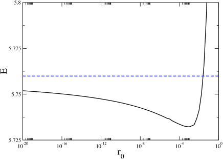
Figure 5: Energy of the ground state of the two dimensional quantum dot with pinning to first order in perturbation theory for $\lambda=3$ and $\hbar=m=\omega=1$, as a function of the radius $r_{0}$. The horizontal line is the equivalent result in the absence of pinning. (color online)

V Bound states in the continuum

We wish now to apply the general results obtained in Section II to the case of the Helmholtz equation on domains which extend to infinity, but consist of wires with crossings and/or bendings. It is well known that in this case the spectrum of the Laplacian contains one or more bound states, depending on the number of crossings and bendings, below the threshold of the continuum. For example, Exner and Seba first showed in Exner89 that a smoothly curved waveguide can support a bound state; Schult et al. have reached a similar conclusion in Schult89 for a different configuration consisting of two crossed wires, of infinite length. Avishai and collaborators have also proved the existence of a bound state in the broken strip configuration for arbitrarily small angles (see Avishai91 ), while Goldstone and Jaffe Jaffe92 have given a variational proof of the existence of a bound state for an infinite tube with bendings in two and three dimensions.

The general results obtained in our Section II suggest that when a number of piercings of infinitesimal radius is added to a crossed wire or to a bent waveguide, the energy of the bound state remains precisely the same although the corresponding wave function changes. If the radius $r_{0}$ of the piercing is now made finite, still one expects the bound state to survive, up to some critical value of $r_{0}$. Notice that the considerations made at the end of Section II also indicate the possibility to extend the same results to filaments inside three dimensional bent tubes.

In this Section we provide an explicit confirmation of our general results, by studying the crossed wire configuration of Ref.Schult89 . In analogy with Ref. Schult89 we have decided to study this problem using two methods: the first method is based on a collocation approach which allows one to obtain a numerical solution to the Helmholtz equation; the second method uses an expansion in a complete set of solutions of the Helmholtz equation on the five domains which compose the global domain (shown in Fig.1 of Ref.Schult89 ). The explicit expressions for these sets of functions may be found in the paper of Schult et al.

Let us first briefly describe the first method. In this case we have discretized the Helmholtz equation on a uniform grid using a set of functions, called Little Sinc Functions (LSF), derived in Ref. Amore07 . These functions have recently been applied in Amore08 to the study of vibration of membranes of arbitrary shapes. Although we refer the reader to Ref. Amore08 for the technical details concerning the implementation of this method, we just mention that the inclusion of piercings inside the domain is handled with extreme simplicity in this approach, provided that the piercing falls on one of the point forming the mesh. As a matter of fact, each LSF is an approximate representation of a Dirac delta function, peaked on one of the points of the mesh: the exclusion of a point from the mesh is therefore obtained by eliminating the corresponding LSF from the set of functions used to discretize the Hamiltonian.

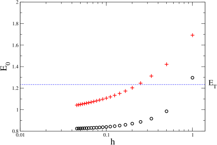
Figure 6: Energy of the ground state of the crossed wired of width $w=1$ calculated using the collocation method as a function of the grid spacing $h$. The circles are the results for the crossed wire without piercing and the crosses are the results for the crossed wire pierced in the origin. The horizontal line is the threshold for the continuum. (color online)

Using the collocation method we have solved numerically the Helmholtz equation on the crossed wire domain, assuming that the arms have a width $w=2$ (we have also set $\hbar=m=1$ in our calculation). Although the arms have infinite extension, we have used arms of finite length $L=10$, in other words we have limited the crossed wire to the interior of a square of sides $20\times 20$. This choice is expected to affect very mildly the lowest energy state which is localized at the crossing. The energy obtained in this way provides in any case an upper bound to the true energy.

In Fig. 6 we display the energy of the ground state obtained numerically with the LSF, for the case of a crossed wire without piercings (circles) and for a crossed wire with a piercing in the origin. The horizontal line is the threshold energy for the continuum. These results are obtained for specific values of the grid spacing, $h$, for which the boundary of the crossed wire falls precisely on the mesh: as discussed in Ref. Amore08 , in this case one obtains a monotonous sequence of values which converge to the exact result from above. We have extracted the continuum limit fitting the two sets of data with

$$E_{0}^{(a)} = a_{0}\ \frac{1+a_{1}h^{a_{2}}}{1+a_{3}h^{a_{4}}}$$ (56)

for the case without piercing and

$$E_{0}^{(b)} = b_{0}\ \frac{1+b_{1}/\log h+b_{2}h^{b_{3}}}{1+b_{4}/\log h+b_{5}h^{b_{6}}}\ ,$$ (57)

for the case with piercing. The coefficients $a_{i}$ and $b_{i}$ are obtained by a least square procedure. The last row of the Table contains the results obtained from the coefficients $a_{0}$ and $b_{0}$ of the fits above using a least square procedure: the results for the two cases are almost degenerate and agree with the result quoted in Ref. Schult89 , i.e. $kw=\frac{w\sqrt{2mE}}{\hbar}\approx 0.812\pi$.

Table 2: Ground state energy of the crossed wire obtained with the collocation method. $E_{0}$ ($E_{0}^{pierced}$) is the energy of the configuration without (with) piercing. The last row are the energies obtained using eqs. (56) and (57) with a least square approach.

$h$	$E_{0}$	$E_{0}^{pierced}$	$h$	$E_{0}$	$E_{0}^{pierced}$
$1$	1.296833	1.692234	$\frac{1}{12}$	0.834904	1.089169
$\frac{1}{2}$	0.985217	1.421753	$\frac{1}{13}$	0.833134	1.081897
$\frac{1}{3}$	0.916621	1.312652	$\frac{1}{14}$	0.831632	1.075505
$\frac{1}{4}$	0.886707	1.246377	$\frac{1}{15}$	0.830342	1.069828
$\frac{1}{5}$	0.870046	1.203231	$\frac{1}{16}$	0.829222	1.064742
$\frac{1}{6}$	0.859464	1.172968	$\frac{1}{17}$	0.828241	1.060153
$\frac{1}{7}$	0.852166	1.150460	$\frac{1}{18}$	0.827374	1.055983
$\frac{1}{8}$	0.846836	1.132966	$\frac{1}{19}$	0.826604	1.052173
$\frac{1}{9}$	0.842779	1.118906	$\frac{1}{20}$	0.825914	1.048673
$\frac{1}{10}$	0.839590	1.107308	$\frac{1}{21}$	0.825294	1.045443
$\frac{1}{11}$	0.837019	1.097539	$\frac{1}{22}$	0.824732	1.042450
LSQ	0.813917	0.813737

Let us now describe the second method. As done in Schult89 we express the solution in each of the five regions as a linear combination of elementary solutions fulfilling the Helmholtz equation:

$$\psi_{I}(x,y) = \sum_{n=0}^{N-1}b_{n}\cosh\frac{\rho_{n}w}{2}e^{\rho_{n}(w/2-x)}\ \cos\frac{(2n+1)\pi y}{w}$$ (58)

$$\psi_{V}(x,y) = \sum_{n=0}^{N-1}b_{n}\left[\cosh\rho_{n}x\ \cos\frac{(2n+1)\pi y}{w}+\cosh\rho_{n}y\ \cos\frac{(2n+1)\pi x}{w}\right]$$ (59)

where $\rho_{n}\equiv\sqrt{\frac{(2n+1)^{2}\pi^{2}}{w^{2}}-\frac{2mE_{0}}{\hbar^{2}}}$. Notice that there is no need of writing the remaining solutions, since they are obtained from $\psi_{I}(x,y)$ by means of rotations and reflections. The unknown coefficients $b_{n}$ are obtained by imposing the continuity of the normal derivative of $\psi(x,y)$ at the border between the regions I and V.Using $N=8$ we have obtained $E=0.849555$ (using as before $w=2$ and $\hbar=m=1$), corresponding to $kw=\frac{w\sqrt{2mE_{0}}}{\hbar}\approx 0.829833\pi$, which is about $2\%$ larger than the result previously obtained (this is consistent with the result found in Avishai91 ).

As we have seen previously the inclusion of a circular piercing is obtained by multiplying the original solution by a factor $\log r/r_{0}$, $r_{0}$ being the radius of the piercing. If this is correct, one should see that, as $r_{0}$ is sent to zero, the energy approaches the value in the absence of piercing.

In Fig. 7 we show the energy of the ground state of the crossed wire with a piercing of radius $r_{0}$ in the origin as a function of $r_{0}$ itself. Using once more a least square procedure we find that in the limit $r_{0}\rightarrow 0$, $E_{0}\approx 0.848$, which is remarkably close to the value without piercing. The critical value of the piercing radius for which the threshold energy is reached is $r_{0}^{crit}\approx 0.0899$. In Fig. 8 we show the wave function of the ground state of the crossed wire with a piercing of radius $r0=10^{-3}$ at the origin, obtained using the expansion in terms of the elementary solutions.

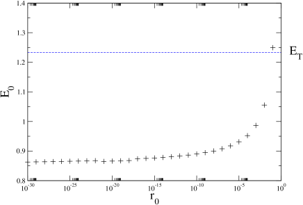
Figure 7: Energy of the ground state of a crossed wire with a piercing in the origin as a function of the radius $r_{0}$. The horizontal line is the threshold of the continuum. (color online)

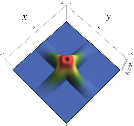
Figure 8: Asymptotic wave function of the ground state of a crossed wire with a piercing of radius $r_{0}=10^{-3}$. (color online)

VI Conclusions

In this paper we have proved that the spectrum of the $d$-dimensional Schrödinger equation does not change when piercings of infinitesimal size are added to the $d$-dimensional domain. The example of the simple harmonic oscillator in $d$ dimensions is worked out and the expected results are obtained both analytically (for a single piercing in the origin) and numerically (up to $20$ piercings). Using these results we have considered a two dimensional parabolic quantum dot and we have calculated the energy of the ground state to first order in perturbation theory, up to the leading finite size correction in the piercing radius. We have found that the interaction energy of the quantum dot is lower for piercings of finite size, and that it can dominate the corresponding finite size correction to the single particle energy above a critical coupling. In our calculations the critical coupling turns out too be large to trust a first order perturbative result. This outcome should motivate a further study of this system, either involving higher order perturbative corrections or a variational calculation, which we hope to carry out soon. Another application considered in the present paper is to configurations supporting bounds states in the continuum, such as wires with crossings and bendings. We have explicitly shown that the inclusion of piercings to these systems does not alter the energy of the ground state, contrary to naive expectations and in perfect accord with our general considerations.

A further remark that we wish to make concerns the Casimir effect on domains with piercings: at least in the case of non interacting fields, and for piercings of infinitesimal size, our results imply that no net effect should appear when piercings are added to a domain. In presence of interactions, whose study is certainly a formidable task, the inclusion of piercings may affect the spectrum thus leading to a net effect.

- (1) J.W.S.Rayleigh, The theory of sound, vol.1, New York; Dover, Second edition (1945)
- (2) C.Y.Wang, Journal of Sound and Vibration 215, 195-199 (1998)
- (3) H.P.W.Gottlieb, Journal of Sound and Vibration 225, 1000-1004 (1999)
- (4) P.A.A.Laura and S.A.Vera, Journal of Sound and Vibration 222, 331-332 (1999)
- (5) P.A.A.Laura,S.L.Malfa, S.A.Vera, D.A.Vega and M.D.Sanchez, Journal of Sound and Vibration 221, 917-922 (1999)
- (6) C.Y.Wang, Journal of Sound and Vibration 234, 363-367 (2000)
- (7) C.Y.Wang, Journal of Sound and Vibration 247, 738-740 (2001)
- (8) L.H.Yu and C.Y.Wang, Journal of Sound and Vibration 239, 363-368 (2001)
- (9) O. Ciftja and A.A. Kumar, Phys. Rev.B 70. 205326 (2004)
- (10) P. Exner and P.Seba, J. Math. Phys. 30, 2574 (1989)
- (11) R.L.Schult, D.G.Ravenall and H.W.Wyld, Phys.Rev.B 39, 5476-5479 (1989)
- (12) Y. Avishai, D. Bessis, B.G. Giraud and G. Mantica, Phys.Rev.B 44, 8028-8034 (1991)
- (13) J.Goldstone and R.L.Jaffe, Phys.Rev.B 45, 14100-14107 (1992)
- (14) L.N.Trefethen and T. Betcke, AMS Contemporary Mathematics, 412, 297-314 (2006)
- (15) P. Amore, M. Cervantes and F.M.Fernández, J. Phys. A 40, 13047-13062 (2007)
- (16) P. Amore, J.Phys. A 41, 265206 (2008)