Simulations of a supersymmetry inspired
model on a fuzzy sphere

Abstract:

We present a numerical study of a two dimensional model of the Wess-Zumino type. We formulate this model on a sphere, where the fields are expanded in spherical harmonics. The sphere becomes fuzzy by a truncation in the angular momenta. This leads to a finite set of degrees of freedom without explicitly breaking the space symmetries. The corresponding field theory is expressed in terms of a matrix model, which can be simulated. We present first numerical results for the phase structure of a variant of this model on a fuzzy sphere. The prospect to restore exact supersymmetry in certain limits is under investigation.

1 The Di Vecchia-Ferrara model

Back in 1977 Di Vecchia and Ferrara introduced an elegant supersymmetric (SUSY) model of the Wess-Zumino type in two dimensions [3]. On a Euclidean plane its action reads

$$S[\phi,\psi]=\frac{1}{2}\int d^{2}x\,\Big{[}\partial_{\mu}\phi\partial_{\mu}\phi+\bar{\psi}\gamma_{\nu}\partial_{\nu}\psi+[V^{\prime}(\phi)]^{2}+\bar{\psi}\psi\,V^{\prime\prime}(\phi)\Big{]}\ ,$$ (1)

where $\phi$ is a scalar field, and $\psi$ is a 2-component Majorana spinor field (with $\bar{\psi}=\psi^{T}C$, where $C=i\sigma_{2}$ is the charge conjugation operator).

We fix the boson-fermion interaction, as well as the bosonic potential, by the choice

$$V(\phi) = \sqrt{\frac{\lambda}{108}}\phi^{3}+\frac{m}{2}\phi^{2}$$ (2)

$$\Rightarrow\quad\frac{1}{2}[V^{\prime}(\phi)]^{2} = \frac{\lambda}{4!}\phi^{4}+m\sqrt{\frac{\lambda}{12}}\phi^{3}+\frac{m^{2}}{2}\phi^{2}\ ,\quad\frac{1}{2}V^{\prime\prime}(\phi)=\sqrt{\frac{\lambda}{12}}\phi+m\ .$$

This action is invariant (up to a total divergence) under the SUSY transformation

$$\left\{\begin{array}[]{ll}\delta\phi=\bar{\epsilon}\psi&\\ \delta\psi=[\gamma_{\nu}\partial_{\nu}\phi-V^{\prime}(\phi)]\epsilon&,\quad\delta\bar{\psi}=\bar{\epsilon}[-\gamma_{\nu}\partial_{\nu}\phi-V^{\prime}(\phi)]\ ,\end{array}\right.$$ (3)

where $\epsilon$ is a constant spinor field.

2 The fuzzy sphere

2.1 Geometry

The coordinate operators $\hat{x}_{i}$ on a fuzzy sphere of radius $R$ have to solve the equation [4]

$$\hat{x}_{1}^{2}+\hat{x}_{2}^{2}+\hat{x}_{3}^{2}=R^{2}1\!\!\!1\ .$$ (4)

This can be achieved by identifying the position operators $\hat{x}_{i}$ with the (re-scaled) angular momentum operators $\hat{L}_{i}\,$,

$$\hat{x}_{i}=\frac{R}{\sqrt{\ell(\ell+1)}}\,\hat{L}_{i}\ ,\qquad i=1,\dots,3\ ,\quad\ell\in{\kern 2.5pt\sf{N}\kern-7.79999pt\sf{I}\kern 7.79999pt\kern-2.5pt}\ ,$$ (5)

where $\ell$ is the spin of the irreducible representation. For finite $\ell$ we obtain $N\times N$ matrices, with $N=\ell+1\,$. Then the coordinate operators on the fuzzy sphere are non-commutative,

$$[\hat{x}_{i},\hat{x}_{j}]={\rm i}\frac{R}{\sqrt{\ell(\ell+1)}}\epsilon_{ijk}\hat{x}_{k}\ .$$ (6)

In the limit $\ell\to\infty$ commutativity is restored, and the sphere is not fuzzy anymore.

2.2 Fields

Some field, for instance our scalar field $\phi(x)$, on the sphere $S^{2}$ can be expanded in term of spherical harmonics $Y_{\ell m}(x)\,$,

$$\phi(x)=\sum_{\ell=0}^{\infty}\,\sum_{m=-\ell}^{\ell}c_{\ell m}Y_{\ell m}(x)\ .$$ (7)

In accordance with the above treatment of the coordinates, we are going to represent also the fields as matrices, so that we end up with a matrix model. Without limiting the matrix size $N$, a Hermitian matrix $\hat{\phi}$ can be expanded in the polarisation tensors $\hat{Y}_{\ell m}$ [5] , in analogy to eq. (7),

$$\hat{\phi}=\sum_{\ell=0}^{\infty}\,\sum_{m=-\ell}^{\ell}c_{\ell m}\hat{Y}_{\ell m}\ .$$ (8)

The polarisation tensors play a rôle analogous to the spherical harmonics. In particular they obey $\hat{L}^{2}\hat{Y}_{\ell m}=\ell(\ell+1)\hat{Y}_{\ell m}\,$, where $\hat{L}^{2}$ is the angular momentum squared (cf. Section 3). Moreover we have the adequate normalisation and parity behaviour, $\frac{4\pi}{N}{\rm Tr}(\hat{Y}_{\ell^{\prime}m^{\prime}}^{\dagger}\hat{Y}_{\ell m})=\delta_{\ell^{\prime}\ell}\delta_{m^{\prime}m}\ ,\ \ \hat{Y}_{\ell m}^{\dagger}=(-1)^{m}\hat{Y}_{\ell-m}\$.

We now introduce a cutoff $\ell_{\rm max}=N-1$, and the remaining coefficients for the field $\phi$ can be embedded into Hermitian $N\times N$ matrices. Thus we arrive at a finite set of degrees of freedom, without any explicit breaking of the space symmetries. Therefore this regularisation is attractive for SUSY models, where the lattice formulation is notoriously troublesome [6]. Moreover the fuzzy sphere regularisation is not plagued by the fermion doubling problem [7].

Theoretical aspects of SUSY on a fuzzy sphere are discussed in Refs. [8] and reviewed in Ref. [9]. The feasibility of numerical simulations in this regularisation has been tested for the $\lambda\phi^{4}$ model in $d=2$ [10] and $d=3$ [11]. For an approach to simulate SUSY gauge theory on the fuzzy sphere, see Ref. [12].

3 The Di Vecchia-Ferrara model on a fuzzy sphere

To be explicit, we transfer the Di Vecchia-Ferrara model from the Euclidean plane to a fuzzy sphere by means of the following substitutions:

$$\phi(x)\ \to\ \hat{\phi} \ ,\quad \frac{1}{4\pi R^{2}}\int_{|x|=R}d\Omega\,\phi(x)\ \to\ \frac{1}{N}{\rm Tr}(\hat{\phi})\ ,$$

$$\partial_{i}\phi(x)\ \to\ \hat{\partial}_{i}\hat{\phi}={\rm i}[\hat{L}_{i},\hat{\phi}] \ ,\quad -\partial^{2}\phi(x)\ \to\ \sum_{i=1}^{3}[\hat{L}_{i},[\hat{L}_{i},\hat{\phi}]]\ ,$$ (9)

where $\hat{\phi}$ is a Hermitian $N\times N$ matrix. We are ultimately interested in the limits $N,\ R\to\infty$.

In practice the left-handed and right-handed applications of the operators can be implemented best by storing the matrix configurations $\hat{\phi}$ as vectors. In this setting the Dirac operator (11) takes the form of a $2N^{2}\times 2N^{2}$ matrix. We symmetrise the fermionic potential as

$$V^{\prime\prime}_{\rm sym}(\hat{\phi})=\frac{1}{2}\Big{(}V^{\prime\prime}(\hat{\phi})\otimes 1\!\!\!1_{N}+1\!\!\!1_{N}\otimes V^{\prime\prime}(\hat{\phi})\Big{)}\ ,$$ (10)

which leads to the Dirac operator

$$D=\left(\begin{array}[]{cc}\hat{\partial}_{3}+\frac{\rm i}{R}1\!\!\!1_{N}+V^{\prime\prime}_{\rm sym}&\hat{\partial}_{-}\\ \hat{\partial}_{+}&-\hat{\partial}_{3}+\frac{\rm i}{R}1\!\!\!1_{N}+V^{\prime\prime}_{\rm sym}\end{array}\right)$$ (11)

with $\hat{\partial}_{\pm}=\hat{\partial}_{1}\pm{\rm i}\hat{\partial}_{2}\,$, and with the representation (9) of the differential operators. As usual in Euclidean space we deal with an anti-Hermitian kinetic part. This also includes the term ${\rm i}/R\,$, which emerges from the curvature effect on the spin connection.

Integrating out the fermionic variables yields the Pfaffian ${\rm Pf}\,[(CD)_{\rm asym}]$, where the subscript means the anti-symmetric part. As a first approach to explore this type of model, we replace the Pfaffian by $\sqrt{{\rm det}\,D}\,$, so we arrive at the matrix model action

$$S[\phi]=\frac{4\pi}{N}{\rm Tr}\Big{(}\frac{1}{2}\sum_{i=1}^{3}[\hat{L}_{i},[\hat{L}_{i},\hat{\phi}]]+\frac{m^{2}}{2}\hat{\phi}^{2}+m\sqrt{\frac{\lambda}{12}}\hat{\phi}^{3}+\frac{\lambda}{4!}\hat{\phi}^{4}\Big{)}-\ln\sqrt{{\rm det}\,D}\ .$$ (12)

4 Order parameters

As in Refs. [10, 11] we are going to explore the phase diagram by considering order parameters, which are constructed from the coefficients $c_{\ell m}$ in the expansion (8). They can be extracted from the relation

$$c_{\ell m}=\frac{4\pi}{N}{\rm Tr}\,[(\hat{Y}_{\ell m})^{\dagger}\hat{\phi}]\ .$$ (13)

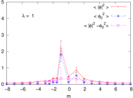
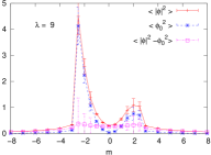
In particular we focus on the quantities

$$\phi_{\ell}^{2}:=\sum_{m=-\ell}^{\ell}|c_{\ell m}|^{2}\qquad{\rm and}\qquad|\phi|^{2}:=\sum_{\ell}\phi_{\ell}^{2}=\frac{4\pi}{N}{\rm Tr}\,[\hat{\phi}^{2}]\ .$$ (14)

Based on the magnitudes of the expectation values $\langle\phi_{0}^{2}\rangle$ and $\langle|\phi|^{2}\rangle$ we distinguish three phases as specified in Table 1, in close analogy to the $\lambda\phi^{4}$ model on a non-commutative flat space [13]:

phase	$\langle\phi_{0}^{2}\rangle$	$\langle|\phi|^{2}\rangle$
disordered	$\approx 0$	$\approx 0$
uniform ordered	$\gg 0$	$\gg 0$
non-uniform ordered	$\approx 0$	$\gg 0$

Table 1: The phases that we observed, along with the respective magnitudes of the order parameters.

• In the disordered phase $\langle\phi_{\ell}^{2}\rangle\approx 0$ holds for all $\ell$. The angular mode decomposition does not detect any contribution that could indicate spontaneous symmetry breaking.

• The uniform ordered phase is characterised by $\langle|\phi|^{2}\rangle\approx\langle\phi_{0}^{2}\rangle\gg 0\,$, i.e. the zero mode contributes significantly, whereas higher modes are suppressed. This phase corresponds to the spontaneous magnetisation in an Ising-type spin model.

• In the non-uniform ordered phase a non-zero mode condenses. This leads to the relations $\langle|\phi|^{2}\rangle\approx\langle|\phi|^{2}-\phi_{0}^{2}\rangle\gg 0\,$. In this case the rotation symmetry is spontaneously broken. That phase is specific to the fuzzy sphere; it does not occur in commutative spaces.

We add that the fuzzy sphere formulation is non-local, as the non-commutativity of the coordinates suggests. Therefore the Mermin-Wagner theorem does not prohibit the non-uniform ordered phase.

5 Numerical results for the phase diagram

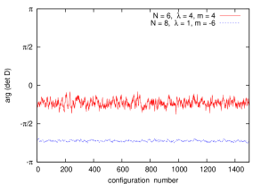
In general the determinant ${\rm det}\,D$ (where $D$ is given in eq. (11)) is complex. In the final limit $N,\,R\to\infty$ it is real positive, however, hence the complex phase represents an artifact of the fuzzy regularisation (apart from the substitution in eq. (12)). We therefore modify the regularisation at this point by using $|{\rm det}\,D|$ already at finite $N$ and $R$. With this modification the action (12) defines a Boltzmann weight which enables Monte Carlo simulations. We performed such simulations with the Metropolis algorithm: in each step, a conjugate pair of matrix elements is updated, and $|{\rm det}\,D|$ is computed explicitly. Throughout our simulations we fixed the radius of the sphere to $R=1$.

So far we simulated at $N=4$, 6 and 8 (which are numerically handled by matrices of size 32, 72 and 128) and we explored the phase diagram in the $(m,\lambda)$ plane. We also measured the phase of the determinant. It turns out to be quite stable, which is favourable for the modified regularisation (in the extreme case of an invariant phase the modification is redundant). Examples for this property are illustrated in Fig. 1.

Figure 1: Two examples for histories of the phase of the fermion determinant. The parameters in these simulations are $N=6,\ \lambda=m=4$ and $N=8,\ \lambda=1,\,m=-6\,$.

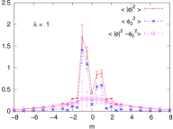
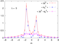
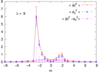
Next we show in Figs. 2 and 3 the expectation values of the order parameters $\langle|\phi|^{2}\rangle$, $\langle\phi_{0}^{2}\rangle$ and $\langle|\phi|^{2}-\phi_{0}^{2}\rangle$ (as discussed in Section 4) for $N=6$ and $N=8$, at $\lambda=1,\,5$ and $9\,$. We actually investigated a larger range of the mass parameter $m\,$, but we show here the interval of interest in view of the phase diagram. In all cases, large values of $|m|$ lead to the disordered phase. When $|m|$ decreases below a critical value $\approx 2$ (which is similar but not identical for both signs of $m$) we enter the phase of uniform order. In the vicinity of $m=0$ we also observe the phase of non-uniform order to set in; the corresponding conditions are given in Table 1.

Figure 2: The order parameters for $N=6$ and $\lambda=1,\,5,\,9$ in the range $m=-8\dots 8$. We see a double peak structure in all cases, and the peak at $m\approx-2$ is enhanced for increasing $\lambda$. A strong coupling $\lambda$ also implies a gradually enlarged phase of non-uniform order.

Figure 3: The order parameters for $N=8$ and $\lambda=1,\,5,\,9$ in the range $m=-8\dots 8$. The phase transitions show a behaviour similar to the results for $N=6$ (Fig. 2), although the values of the order parameters differ.

For $N=6$ and 8 we probed $\lambda=1,\dots,10\,$, which gives rise to the phase diagram in Fig. 4.

Figure 4: The phase diagram at $N=6$ and $8$, which is identified from measurements as shown in Figs. 2 and 3 for $\lambda=1,\,2,\ \dots,10$.

6 Conclusions

We explored a new way to simulate a two dimensional model of the Wess-Zumino type. The model is wrapped on a sphere and the fields are expanded in spherical harmonics. A truncation in the angular momentum renders the sphere fuzzy, and the corresponding field coefficients build a finite set of degrees of freedom to be used in numerical simulations. In this first approach we simplified the Pfaffian to $\sqrt{{\rm det}D}$. Thus we studied a SUSY inspired system of interacting scalars and Majorana fermions on a fuzzy sphere.

In the final limit of infinite angular momentum cutoff $N$ and radius $R$, the determinant ${\rm det}D$ is real positive. This does not hold at finite $N$ and $R$, so we modify the regularisation by employing the modulus of the fermion determinant already on the regularised level. We expect this formulation to lead to the same limit. This expectation is supported by the observation that the fluctuations of the phase $\,{\rm arg}({\rm det}D)\,$ are small.

With this method we simulated the system at $N=4$, $6$ and $8$ and $R=1$. The basic properties are similar in all cases; in particular large $|m|\mathop{\raise 1.29167pt\hbox{$>$\kern-7.5pt\raise-4.73611pt\hbox{$\sim$}}}2$ always leads to a disordered phase. So it is conceivable that we are already peeping at aspects of the large $N$ limit. However, the final stabilisation of the phase diagram at large $N$ may involve a re-scaling of the axes.

The ordered non-uniform phase emerges as a consequence of the non-commutativity of the coordinates, which we use on the regularised level. We observed that phase around $m\approx 0$, and it ought to evaporate as we proceed to larger $N$. That feature is left for further investigation.

Although this project is still on-going, the preliminary results are encouraging regarding the hope to find a way to formulate and explore SUSY inspired models beyond perturbation theory.

Acknowledgements : This work is based on collaboration with D. O’Connor, M. Panero and J. Volkholz. J.V. presented this talk, but meanwhile he left physics and he preferred to withdraw his name. I am also indebted to A. Balachandran, J. Medina, A. Wipf and B. Ydri for helpful discussions. Most computations were performed on clusters of the “Norddeutscher Verbund für Hoch- und Höchstleistungsrechnen” (HLRN).

References

- [1]
- [2]
- [3] P. Di Vecchia and S. Ferrara, Nucl. Phys. B 130 (1977) 93.
- [4] J. Madore, Class. and Quant. Grav. 9 (1992) 69.
- [5] D.A. Varshalovich, A.N. Moskalev and V.K. Khersonky, Quantum Theory of Angular Momentum: Irreducible Tensors, Spherical Harmonics, Vector Coupling Coefficients, 3nj Symbols, World Scientific, Singapore (1998).
-
[6]
See for a review: A. Feo
Nucl. Phys. (Proc. Suppl.) 119 (2003) 198,
and contributions to these procs.:
S. Arianos, A. D’Adda, N. Kawamoto and J. Saito,
PoS(LAT2007)259. S. Catterall and T. Wiseman,
PoS(LAT2007)051. A. D’Adda, I. Kanamori, N. Kawamoto and K. Nagata,
PoS(LAT2007)271.
H. Fukaya, I. Kanamori, H. Suzuki and T. Takimi, PoS(LAT2007)264. T. Kästner, G. Bergner,
S. Uhlmann, A. Wipf and C. Wozar, PoS(LAT2007)265. J. Nishimura, K.N. Anagnostopoulos,
M. Hanada and S. Takeuchi, PoS(LAT2007)059. K. Ohta and T. Takimi, PoS(LAT2007)279. - [7] A.P. Balachandran and G. Immirzi Phys. Rev. D 68 (2003) 065023.
[8]
H. Grosse, C. Klimčík and P. Prešnajder,
Commun. Math. Phys. 185 (1997) 155.
H. Grosse and G. Reiter, J. Geom. Phys. 28 (1998) 349.
C. Klimčík, Commun. Math. Phys. (1999) 206 567.
A.P. Balachandran, S. Kürkçüoǧlu and E. Rojas,
JHEP 0207 (2002) 056.
A.P. Balachandran, A. Pinzul and B. Qureshi,
JHEP 0512 (2005) 002.
B. Ydri, Int. J. Mod. Phys. A 22 (2007) 5179;
Mod. Phys. Lett. A 22 (2007) 2565. - [9] A.P. Balachandran, S. Kürkçüoǧlu and S. Vaidya, hep-th/0511114.
- [10] X. Martin, JHEP 0404 (2004) 077. F. Garcia Flores, D. O’Connor and X. Martin, PoS(LAT2005)262. M. Panero, JHEP 0705 (2007) 082; SIGMA 2 (2006) 081. C.R. Das, S. Digal and T.R. Govindarajan, arXiv:0706.0695 [hep-th]; arXiv:0801.4479 [hep-th].
- [11] J. Medina, W. Bietenholz, F. Hofheinz and D. O’Connor, PoS(LAT2005)263; JHEP 04 (2008) 041. J. Medina, Ph.D. Thesis, CINVESTAV, México D.F. (2006) [arXiv:0801.1284 [hep-th]].
- [12] K.N. Anagnostopoulos, T. Azuma, K. Nagao and J. Nishimura, JHEP 0509 (2005) 046.
- [13] W. Bietenholz, F. Hofheinz and J. Nishimura, Nucl. Phys. (Proc. Suppl.) 119 (2003) 941; Acta Phys. Pol. B 34 (2003) 4711; JHEP 06 (2004) 042. F. Hofheinz, Ph.D. Thesis at Humboldt-Universität zu Berlin (2003), published in Fortsch. Phys. 52 (2004) 391. A. Bigarini, Ph.D. Thesis at Università degli Studi di Perugia (2005). J. Volkholz, Ph.D. Thesis at Humboldt-Universität zu Berlin (2007).