Sound waves in the intracluster medium of the Centaurus cluster
Abstract
We report the discovery of ripple-like X-ray surface brightness oscillations in the core of the Centaurus cluster of galaxies, found with 200 ks of Chandra observations. The features are between 3 to 5 per cent variations in surface brightness with a wavelength of around 9 kpc. If, as has been conjectured for the Perseus cluster, these are sound waves generated by the repetitive inflation of central radio bubbles, they represent around of spherical sound-wave power at a radius of 30 kpc. The period of the waves would be yr. If their power is dissipated in the core of the cluster, it would balance much of the radiative cooling by X-ray emission, which is around within the inner 30 kpc. The power of the sound waves would be a factor of four smaller that the heating power of the central radio bubbles, which means that energy is converted into sound waves efficiently.
keywords:
X-rays: galaxies — galaxies: clusters: individual: Centaurus cluster — intergalactic medium — cooling flows1 Introduction
Ripples in the X-ray surface brightness of galaxy clusters were first discovered in the Perseus cluster of galaxies (Fabian et al., 2003). As the surface brightness is roughly proportional to the density of the intracluster medium (ICM) squared, these are density ripples.
Fabian et al. (2003) explained these variations as sound waves generated by the inflation of the bubbles of relativistic plasma in the core of the cluster by the central active nucleus. Providing that these sound waves can be dissipated as they travel (Fabian et al., 2005a), they have the ability to transport energy from the central nucleus to the core of the cluster. If they carry significant quantities of energy, they may provide the distributed heating required (Voigt & Fabian, 2004) to prevent large quantities of the ICM from cooling (Peterson & Fabian, 2006; McNamara & Nulsen, 2007). Subsequent theoretical work (Ruszkowski et al., 2004; Sijacki & Springel, 2006) have shown that sound waves may be able to help heat the cores of clusters in a gentle distributed fashion.
A deep 900 ks observation of Perseus showed the ripples in exquisite detail enabling their amplitude to be measured (Fabian et al., 2006). Subsequently, we used the amplitude of the ripples to calculate the amount of energy propagated in them if they are sound waves (Sanders & Fabian, 2007). They would carry enough energy in Perseus to combat a significant fraction of the cooling rate, and appear to decline in power with radius.
The Perseus observations also reveal thick spherical shells around each inner bubble at a higher gas density and pressure than their surroundings. These high pressure shells have a sharp outer edge where the density abruptly jumps by about 30 per cent, and is interpreted as a weak shock. We have assumed that such high pressure regions propagate outward to become the ripples. A problem with the weak shock interpretation is that there is no temperature jump coincident with the density one. The observed limit on any jump in temperature is inconsistent with an adiabatic shock. The region has been studied and discussed in detail by Graham et al. (2008b). It is noted there that the Northern optical filaments of cold gas stop at the shock front, so cold gas is likely being mixed with the hot gas there due to turbulence generated at that front. This could explain a reduction in temperature of the post shock gas.
Sound waves or ripples have not been detected in other systems. However, they may still be an important contribution to the heating processes in clusters as they could be difficult to detect. They were not found until 200 ks of Chandra time of the Perseus cluster was obtained. Perseus is the X-ray brightest galaxy cluster by a factor of 1.7 (in the 2-10 keV band; Edge et al. 1990). Clearly the detectability of ripples will vary with cluster surface brightness and observation time. It will also vary with ripple amplitude and wavelength and with cluster properties. These effects have been examined numerically by Graham et al. (2008a), finding that it is difficult to observe these features with current instruments in clusters other than Perseus. The detectability of ripples, however, depends on unknown factors, such as the wavelength and amplitude of the ripples. These factors can be estimated with a large degree of uncertainty from the properties of the cluster, assuming that they are responsible for heating the cluster core and have a wavelength similar to the bubble size.
Here we report on some ripples which we find in a 200 ks Chandra observation of the Centaurus cluster of galaxies. These data were examined previously by Fabian et al. (2005b) and Sanders & Fabian (2006a), examining the thermal distribution of gas in the cluster core and its metallicity.
The Centaurus cluster of galaxies is a nearby (; Lucey et al. 1986) X-ray bright galaxy cluster (; Edge et al. 1990). It contains a low radiative efficiency nucleus (Taylor et al., 2006) and distinct bubbles of relativistic plasma (Taylor et al., 2002) displacing the intracluster medium, as seen by Chandra (Sanders & Fabian, 2002).
We assume , which translates into scale of 213 pc per arcsec.
2 Data analysis
We obtained Chandra observations with IDs 504, 4954, 4955 and 5310. Each of these observations used the ACIS-S detector aimed at the central X-ray peak of Centaurus. Exposure maps for each of the observations and for each of the detector CCDs were created with the ciao mkexpmap tool, binning the detector pixels by a factor of 2 and leaving the observation time factor in the map by disabling normalization. We used the appropriate bad pixel maps and attitude files to create these maps and assumed a monochromatic energy of 1.5 keV. We created images of Centaurus for each observation and detector between 0.5 and 6 keV from the event files with the same spatial binning. We added all the images together to make a total image, and all the exposure maps to make a total exposure map. A total exposure-corrected image was created by dividing the total image by total exposure map.
2.1 Fourier filtering
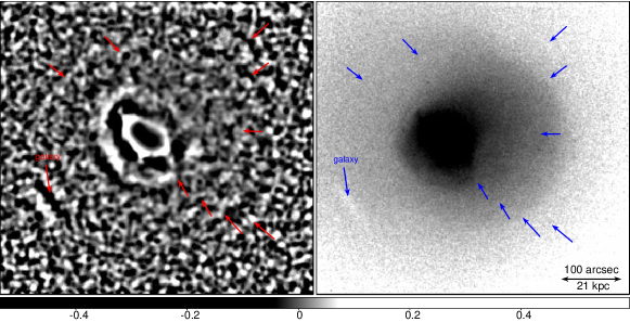
To search for features in the exposure-corrected image we used a Fast Fourier Transform (FFT) high-pass filter as in Sanders & Fabian (2007). The filter removes smooth underlying cluster emission and so is similar to the unsharp-mask method. Firstly, we truncated the exposure-corrected values in the image to reduce the level of the bright emission in the cluster centre. This was done because using Fourier filters on bright peaks can introduce ‘fringes’ on the filtered image, which may look like additional ripples. We tested that the features in the image were robust with different clipping and filtering parameters. We also removed point sources from the image before filtering, by selecting them by eye, then replacing the source pixels with values selected randomly from the values of the surrounding pixels.
In our analysis we removed spatial frequencies longer than 10 per cent of the size of the image ( arcsec pixels square), allowing through all frequencies shorter than 5 per cent of the size of the image. We allowed intermediate frequencies through the filter with a linear filter between these two threshold spatial frequencies. We then computed the ratio between the filtered map and the original image, after smoothing by a 20 arcsec Gaussian, to allow the features in the centre and outskirts to be seen. The filtered image and a smoothed unfiltered image are shown in Fig. 1.
2.2 Surface brightness profiles
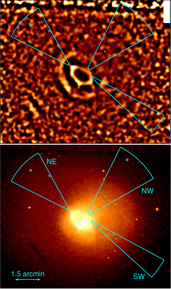
To verify that the features that we have found are not artifacts produced by the Fourier filtering technique and to measure the amplitude of the features, we created surface brightness profiles in different sectors. In Fig. 2 we show the sectors used to make the profiles. Note that the sectors are not centred on the active nucleus, but are centred so that the surface brightness features are aligned with the radial bins.
To produce a profile we take a sector and split it into radial bins. From each bin we count the number of counts from each of the separate observations in the 0.5 to 6 keV band. We also take the average value of the total exposure map in each bin (single-pixel binned exposure maps are used in this part of the analysis) and multiply by the area of the bin in pixels. We divide the total number of counts by the total exposure map value to make a surface brightness measurement. Point sources were removed from the regions by eye. Note that as the profiles are centred to match the ripples, the radii in the profiles do not correspond to the same radius in the cluster.
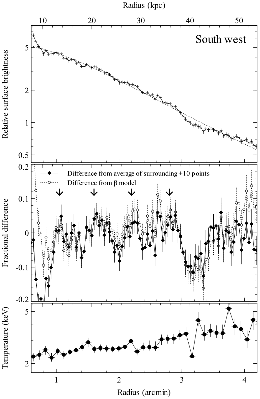
We plot the profile in the sector towards the south west in Fig. 3. Shown in the top of the panel is a surface brightness profile in 120 equal-width (0.04 arcmin) radial bins. We also plot a -model fit to the surface brightness profile in the radial range shown. In the lower panel we show the fractional residuals from the data to the model. In addition we show the fractional residuals of the surface brightness of each bin to the average of the 10 bins inside and outside of that bin (excluding bins beyond the edge of the profile). The two different sets of residuals are similar. We only show the residuals from the averaging technique in later profiles here, as it is more difficult to fit a smooth profile to these other sectors. The averaging method appears to be robust. Note how the surface brightness significantly oscillates around the zero value. There are strong positive features around 1.05, 1.6, 2.2, and 2.8 arcmin in radius (plotted as arrows). The feature in the image at 3.6 arcmin is seen at low significance in this profile, but only a small part of it is captured here. The large negative feature at 3.2 arcmin is the sharp drop in surface brightness seen in the right-hand panel in Fig. 1. The amplitude of the variation is typically of the order of 4 or 5 per cent. An estimate for the wavelength of the features is around 0.7 arcmin (9 kpc).
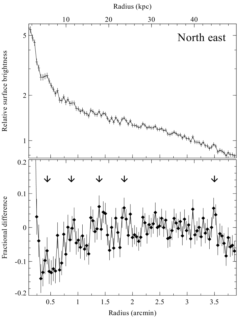
We show in Fig. 4 the north east sector profile generated in 100 equal-width (0.038 arcmin) bins and the fractional residuals from the surrounding bins. In this image we see positive features at 0.44, 0.88, 1.39, 1.85 and 3.5 arcmin. All of these enhancements are seen in the FFT-filtered image. The inner peak may be associated with the edge of the possible radio bubble seen as a low pressure region by Crawford et al. (2005).
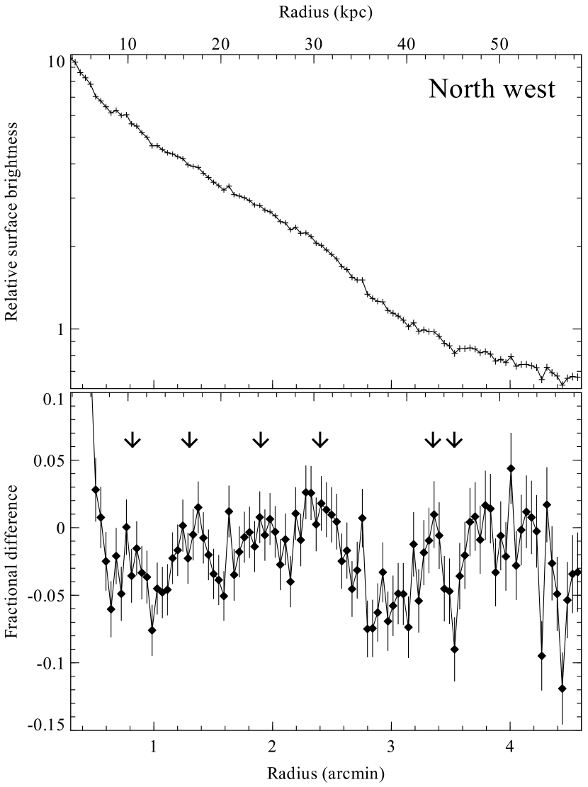
Our final surface brightness profile is a sector towards the north west of the cluster core (Fig. 5). There are around four sets of obvious peaks in the inner part of the cluster, at radii of 0.82, 1.3, 1.9 and 2.4 arcmin. There is also another peak at 3.35 arcmin, followed by a sharp drop (as seen in the FFT-filtered image) at 3.53 arcmin, then another rise upwards. The size of the variations in this sector appear smaller than the other two, with an amplitude of around 3 per cent.
2.3 Temperature variations
If the ripples are due to adiabatic sound waves, then temperature fluctuations are expected at about one third of the relative amplitude of the surface brightness variations. The amplitude of the temperature fluctuations should therefore be 1–2 per cent in both the Perseus and Centaurus clusters. It is not clear whether this is consistent with the range seen in the Perseus cluster (Sanders & Fabian, 2007; Graham et al., 2008b), although the multiphase nature of the gas means that there are systematic uncertainties at the same level which preclude any definitive measurement. For the Centaurus cluster the uncertainties on the temperature are larger (Fig. 3) and no detection is possible at this level with current data.
2.4 Projection effects
To compute the real amplitude of the ripples in the absence of projection effects in the Perseus cluster, we simulated projected profiles of ripples with a known amplitude on an emissivity model. Here we compare this method with another where we directly deproject the surface brightness profile.
Starting from the outer radial bin in a sector, the surface brightness is converted to an emissivity, assuming that all the emission comes from a shell with those radii. The method examines successively interior bins, subtracting off the contribution to the projected emission from outer shells, converting the surface brightness to an emissivity. To calculate the uncertainties on the emissivity profile a Monte Carlo method is used. The input profiles are perturbed by drawing from a Gaussian distribution using the best fitting values as the central value, and uncertainties as widths. The deprojection is repeated many times. The emissivity from the median iteration and 84.2 and 15.8 percentiles are used to calculate the emissivity of a bin and its uncertainty. The assumption of this method is that the cluster is spherically symmetrical.
Using this deprojection technique, we obtain a ratio between the projected surface brightness and the emissivity after deprojection of around 4. This is consistent with a factor of 5, computed using a numerical model where we integrate a cluster emissivity model along the line of sight (using a sinusoid with wavelength of 0.7 arcmin on a power law emissivity profile with an index of -1.6). Therefore the density variations are around 2.5 times the surface brightness variations. 3 to 5 per cent surface brightness variations translate to 7.5 to 12.5 per cent density variations.
3 Discussion
Linear features in exposure-corrected images can be caused by inaccurate exposure correction, for instance, bad pixels not properly accounted for, or a variation of spectrum with source position. We believe none of the features in the images presented are exposure-correction artifacts, as the constituent exposure maps have no features aligned in the same direction. Any artifacts in the images should by aligned with the edge of the CCDs or the readout direction. Most of the ripples also appear to have curvature, which artifacts would not.
The Fourier filtering process can introduce spurious ripple-like features. We have tested that the features are robust in the image presented by trying different filtering levels. The surface brightness profiles, which have no Fourier filtering applied, clearly demonstrate that the ripples are real features.
Rather than pressure waves in the ICM, another mechanism which can give surface brightness variations are fluctuations in the metallicity of the ICM. The ICM can contain high metallicity blobs a few kpc in size (Sanders & Fabian, 2007) and metallicity map of Centaurus is not smooth (Fabian et al., 2005b). In order to check that metallicity is not the cause of the observed ripples, we compared the spectra in the south-western sector between radii of 1.53 and 1.86 arcmin, where there is excess surface brightness, and 1.86 and 2.15 arcmin, where there is a deficit. The spectra and the strength of the iron line were very similar, with no significant differences in temperature or metallicity measured by spectral fitting. In this case the region with the brightness deficit was slightly higher in metallicity by . As a function of radius the brightness peaks correlate with emission measure, not temperature or metallicity. In neither the Perseus nor Centaurus clusters do the observed metallicity variations in a metallicity map correlate with the observed surface brightness ripples.
To the west of the cluster at a radius of 30 kpc (2.3 arcmin), the deprojected electron density is around and the temperature is 2.5 keV (Sanders & Fabian, 2006b). The mean radiative cooling time, , is 3.3 Gyr at this radius. Using equation (3) of Sanders & Fabian (2007), the pressure ripples have a height for 10 per cent density ripples, assuming . 10 per cent density ripples would correspond to a Mach number of 1.07. The pressure amplitude translates into a spherical sound wave power at this radius, , were is the radius, is the mass density and is the sound speed (the factor of 2 converts from amplitudes to RMS energy). A 9 kpc wavelength corresponds to a wave period of yr. This period is close to that inferred for the ripples in the Perseus cluster (Fabian et al., 2003).
If we choose a radius of 15 kpc instead (1.2 arcmin, where ), the electron density is and the temperature is 2.0 keV. 10 per cent density ripples translate into of wave power.
If the inner features are 5 per cent surface brightness instead of 4, the power is boosted by around 60 percent. The numbers are uncertain by a factor of a few due to the assumptions of spherical symmetry and the true projection factor. The ripples are not simple monochromatic waves with a single wavelength.
The power in the sound waves can be compared to the bolometric luminosity of the core of the cluster. If we fit the Chandra spectrum from the inner 15 kpc of Centaurus with a model made up of multiple temperature components of 0.5, 1, 2, 4 and 8 keV, we obtain a bolometric X-ray luminosity of , when absorption is removed. From the inner 30 kpc, we obtain a luminosity of . Similar luminosities are obtained from a grating spectrum of the core of the cluster (Sanders et al., 2008), although the geometry on the sky makes comparisons difficult. The luminosity of the core is just over twice the wave power calculated above. Therefore the sound waves are close to what is required to combat cooling in the core of the cluster.
If we assume that the two inner radio bubbles contain of energy and that they deposit this energy over the period of the sound waves ( yr), we estimate they have a total heating power of . This is four times the power we infer from the ripples. This means that the conversion of jet power via bubbles into sound waves is remarkably efficient (). Graham et al. (2008b) find that the energy in the high pressure region around the bubbles in the Perseus cluster is about . These observational results mean that the energy content of the radio bubbles is close to the energy injected by the nucleus, contrary to the interpretation by Binney et al. (2007) of the simulations of Omma & Binney (2004), where only about 10 per cent of the jet energy was found to go into the bubbles.
4 Conclusions
We detect surface brightness deviations in a Chandra image of the Centaurus cluster of galaxies. These features are between 3 and 5 per cent in size. Assuming that they are sound waves, the wave power is approximately in the inner 30 kpc, with a period of yr and a wavelength of 9 kpc. The power is close to the X-ray luminosity of this central region. It is therefore energetically possible that sound waves are the mechanism by which the power of the central black hole is transmitted quasi-isotropically through the cluster. Provided that the power in the waves is gradually dissipated as heat, they provide the means by which radiative cooling is balanced by heating in the inner cluster core.
Acknowledgements
ACF acknowledges the Royal Society for support.
References
- Binney et al. (2007) Binney J., Bibi F. A., Omma H., 2007, MNRAS, 377, 142
- Crawford et al. (2005) Crawford C. S., Hatch N. A., Fabian A. C., Sanders J. S., 2005, MNRAS, 363, 216
- Edge et al. (1990) Edge A. C., Stewart G. C., Fabian A. C., Arnaud K. A., 1990, MNRAS, 245, 559
- Fabian et al. (2005a) Fabian A. C., Reynolds C. S., Taylor G. B., Dunn R. J. H., 2005a, MNRAS, 363, 891
- Fabian et al. (2003) Fabian A. C., Sanders J. S., Allen S. W., Crawford C. S., Iwasawa K., Johnstone R. M., Schmidt R. W., Taylor G. B., 2003, MNRAS, 344, L43
- Fabian et al. (2005b) Fabian A. C., Sanders J. S., Taylor G. B., Allen S. W., 2005b, MNRAS, 360, L20
- Fabian et al. (2006) Fabian A. C., Sanders J. S., Taylor G. B., Allen S. W., Crawford C. S., Johnstone R. M., Iwasawa K., 2006, MNRAS, 366, 417
- Graham et al. (2008a) Graham J., Fabian A. C., Sanders J. S., 2008a, MNRAS, submitted
- Graham et al. (2008b) Graham J., Fabian A. C., Sanders J. S., 2008b, MNRAS, 386, 278
- Lucey et al. (1986) Lucey J. R., Currie M. J., Dickens R. J., 1986, MNRAS, 221, 453
- McNamara & Nulsen (2007) McNamara B. R., Nulsen P. E. J., 2007, ARA&A, 45, 117
- Omma & Binney (2004) Omma H., Binney J., 2004, MNRAS, 350, L13
- Peterson & Fabian (2006) Peterson J. R., Fabian A. C., 2006, Phys. Rep., 427, 1
- Ruszkowski et al. (2004) Ruszkowski M., Brüggen M., Begelman M. C., 2004, ApJ, 611, 158
- Sanders & Fabian (2002) Sanders J. S., Fabian A. C., 2002, MNRAS, 331, 273
- Sanders & Fabian (2006a) Sanders J. S., Fabian A. C., 2006a, MNRAS, 371, 1483
- Sanders & Fabian (2006b) Sanders J. S., Fabian A. C., 2006b, MNRAS, 370, 63
- Sanders & Fabian (2007) Sanders J. S., Fabian A. C., 2007, MNRAS, 381, 1381
- Sanders et al. (2008) Sanders J. S., Fabian A. C., Allen S. W., Morris R. G., Graham J., Johnstone R. M., 2008, MNRAS, 385, 1186
- Sijacki & Springel (2006) Sijacki D., Springel V., 2006, MNRAS, 366, 397
- Taylor et al. (2002) Taylor G. B., Fabian A. C., Allen S. W., 2002, MNRAS, 334, 769
- Taylor et al. (2006) Taylor G. B., Sanders J. S., Fabian A. C., Allen S. W., 2006, MNRAS, 365, 705
- Voigt & Fabian (2004) Voigt L. M., Fabian A. C., 2004, MNRAS, 347, 1130