A Moving Bump in a Continuous Manifold:
A Comprehensive Study of the Tracking Dynamics of Continuous Attractor Neural Networks

C. C. Alan Fung1, K. Y. Michael Wong1 and Si Wu2,3
1Department of Physics, Hong Kong University of Science and Technology,
Clear Water Bay, Hong Kong, China
2Department of Informatics, University of Sussex, Brighton, United Kingdom
3Lab of Neural Information Processing, Institute of Neuroscience, Shanghai, China
Abstract

Understanding how the dynamics of a neural network is shaped by the network structure, and consequently how the network structure facilitates the functions implemented by the neural system, is at the core of using mathematical models to elucidate brain functions. This study investigates the tracking dynamics of continuous attractor neural networks (CANNs). Due to the translational invariance of neuronal recurrent interactions, CANNs can hold a continuous family of stationary states. They form a continuous manifold in which the neural system is neutrally stable. We systematically explore how this property facilitates the tracking performance of a CANN, which is believed to have clear correspondence with brain functions. By using the wave functions of the quantum harmonic oscillator as the basis, we demonstrate how the dynamics of a CANN is decomposed into different motion modes, corresponding to distortions in the amplitude, position, width or skewness of the network state. We then develop a perturbative approach that utilizes the dominating movement of the network’s stationary states in the state space. This method allows us to approximate the network dynamics up to an arbitrary accuracy depending on the order of perturbation used. We quantify the distortions of a Gaussian bump during tracking, and study their effects on the tracking performance. Results are obtained on the maximum speed for a moving stimulus to be trackable and the reaction time for the network to catch up with an abrupt change in the stimulus.

1 Introduction

The brain performs computation by updating its internal states according to dynamical rules that are determined by both the nature of external inputs and the structure of neural networks. A neural system acquires its network structure through either learning from experience, or inheriting from evolution or both. Its impact on network dynamics is twofold: on one hand, it determines the stationary states of the network that lead to associative memory; and on the other hand, it carves the landscape of the state space of the network as a whole, which may contribute to other cognitive functions, such as movement control, spatial navigation, population decoding and object categorization. Understanding how the dynamics of a neural network is shaped by its network structure is at the core of using mathematical models to elucidate brain functions [Dayan and Abbott 2001].

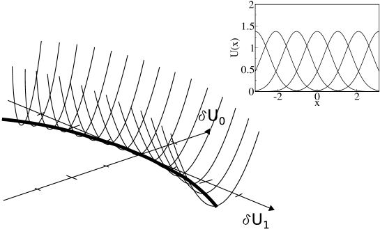
Associative memories, such as those based on the Hopfield model [Hopfield 1984, Domany, van Hemmen, and Schulten 1995], have been intensively studied over the past decades. However, an equally important issue has not been investigated to the same extent, namely, how a large-scale structure of the state space of a neural system may facilitate brain functions. Recently, a type of recurrent network, called continuous attractor neural networks (CANNs), has received wide attention [Wilson and Cowan 1972, Amari 1977, Georgopoulos, Kalaska, Caminiti, and Massey 1982, Maunsell and Van Essen 1983, Funahashi, Bruce, and Goldman-Rakic 1989, Wilson and McNaughton 1993, Rolls, Robertson, and Georges-Francois 1995, Ben-Yishai, Lev Bar-Or, and Sompolinsky 1995, Zhang 1996, Seung 1996, Samsonovich and McNaughton 1997, Camperi and Wang 1998, Ermentrout 1998, Hansel and Sompolinsky 1998, Taube 1998, Deneve, Latham, and Pouget 1999, Wang 2001, Laing and Chow 2001, Wu, Amari, and Nakahara 2002, Stringer, Trappenberg, Rolls, and Aranjo 2002, Brody, Romo, and Kepecs 2003, Erlhagen 2003, Gutkin, Pinto, and Ermentrout 2003, Renart, Song, and Wang 2003, Trappenberg 2003, Folias and Bressloff 2004, Wu and Amari 2005, Chow and Coombes 2006, Miller 2006, Machens and Brody 2008, Wu, Hamaguchi, and Amari 2008]. These models are particularly useful when modeling the encoding of continuous stimuli in neural systems. Different from other attractor models, CANNs have a distinctive feature that their neuronal interactions are translationally invariant. As a result, they can hold a family of stationary states that can be translated into each other without the need to overcome any barriers. In the continuum limit, these stationary states form a continuous manifold111A manifold is a mathematical concept. Simply stated, it is a set of points with a coordinate system. Here, each stationary state of the network is a point in the manifold. As will be shown later, these stationary states have the shape of a Gaussian bump, and their peak positions define the coordinates. in which the system is neutrally stable, and the network state can translate easily when the external stimulus changes continuously. Beyond pure memory retrieval, this large-scale structure of the state space endows the neural system with a tracking capability. An illustration of the landscape of the state space of a CANN and how it leads to neutral stability of the network stationary states is shown in Fig. 1.

The tracking dynamics of a CANN has been theoretically studied by several authors in the literature (see, e.g.,[Ben-Yishai, Lev Bar-Or, and Sompolinsky 1995, Zhang 1996, Samsonovich and McNaughton 1997, Xie, Hahnloser, and Seung 2002, Folias and Bressloff 2004, Wu and Amari 2005]). These studies have demonstrated clearly that a CANN has the capacity of tracking a moving stimulus continuously and that this tracking property can describe many brain functions well. Detailed rigorous analyses of the tracking behaviors of a CANN are still lacking, however, including, for instance, 1) the conditions under which a CANN can track a moving stimulus successfully; 2) how the network state is distorted during the tracking; and 3) how these distortions affect the tracking performance of a CANN. In this study, we systematically investigate these issues.

We use a simple, theoretically solvable model of a CANN as the working example. The stationary states of the network have a Gaussian shape, and the network dynamics can be described using the basis functions of quantum harmonic oscillators. These analytical results allow us to explore the tracking performances of a CANN in much more detail than in previous studies based on simulation observations. In particular, we demonstrate clearly how the dynamics of a CANN is decomposed into different modes corresponding to distortions in the height, position, width or skewness of the network bump states. Their contributions to the tracking performance are determined by the amplitudes of the corresponding eigenvalues of the neuronal interaction kernel. For a CANN, neutral stability implies that the mode of positional shift dominates the network dynamics and that other modes have high-order contributions. From this property, we develop a time-dependent perturbative approach to simplify the network dynamics. Geometrically, this corresponds to projecting the network dynamics on its dominating motion modes. The solution of the perturbation method is expressed in a simple closed form, and we can approximate the network dynamics up to an arbitrary accuracy depending on the order of perturbation used. With this method, we explore two tracking performances of a CANN, namely, the condition under which the network can successfully track a moving stimulus and the reaction time for the network to catch up with sudden changes in the stimulus. Both properties are associated with the unique dynamics of a CANN and can be tested in practice.

The idea of utilizing the special structure of a CANN to simplify its dynamics has also been reported in other studies. Wu et al projected the dynamics of a CANN on its single dominating motion mode, the tangent of the attractor space, and simplify the network dynamics into a one-dimensional equation [Wu, Hamaguchi, and Amari 2008]. Several other authors also proposed different approaches to simplifying the network dynamics  [Ben-Yishai, Lev Bar-Or, and Sompolinsky 1995, Wennekers 2002, Renart, Song, and Wang 2003, Miller 2006]. Compared with these studies, our contributions are that: 1) we elucidate the tracking behavior of a CANN in much more detail, particularly the effect of distortions in the network state on the tracking performance and the development of a perturbative method to systematically improve the description of the network dynamics; 2) we predict on the tracking behavior of a CANN, namely, the maximum speed for a moving stimulus to be trackable by the network [Hansel and Sompolinsky 1998] and the logarithmic nature of the reaction time; and 3) we also analytically investigate the tracking dynamics of a two-dimensional CANN. We expect that the mathematical framework developed in this work will have wide applications in the theoretical study of CANNs.

The organization of the paper is as follows. In Section 2, the unique dynamics of a CANN is explored, and we demonstrate how a CANN is decomposed into different modes. In Section 3, a simple method of projecting the network dynamics onto its single primary motion mode, i.e., the tangent of the manifold formed by all stationary states, is used to investigate the tracking performance of a CANN. In Section 4, a perturbative approach is developed to systematically improve the description of the tracking dynamics of the network. The effects of the shape distortions of the network state on the tracking dynamics are described. In Section 5, the dynamics of a two-dimensional CANN is investigated. In Section 6, we present the discussion and conclusions. The mathematical details are presented in the appendices. Preliminary results have been published in [Fung, Wong, and Wu 2008].
Refer to caption
Figure 1: The energy landscape of the state space of a CANN. A canyon is formed by projecting the stationary states onto the subspace formed by δU1𝛿subscript𝑈1\delta U_{1} and δU0𝛿subscript𝑈0\delta U_{0}, i.e., the position and the height distortions of the network states. Motion along the canyon corresponds to the positional shift of the bump (inset).

2 Intrinsic Dynamics of a CANN

Let us consider a one-dimensional continuous stimulus x𝑥x encoded by an ensemble of neurons. For example, the stimulus may represent the direction of movement, the orientation or a general continuous feature of objects extracted by the neural system. We consider the range of possible values of the stimulus being much larger than the range of neuronal interactions. We can thus effectively take x(,)𝑥x\in(-\infty,\infty).

Let U(x,t)𝑈𝑥𝑡U(x,t) be the synaptic input at time t𝑡t to the neurons whose preferred stimulus is x𝑥x, and let r(x,t)𝑟𝑥𝑡r(x,t) be the firing rate of these neurons. r(x,t)𝑟𝑥𝑡r(x,t) increases with the synaptic input, but saturates in the presence of global activity-dependent inhibition. A solvable model that captures these features is given by the divisive normalization [Deneve, Latham, and Pouget 1999, Wu, Amari, and Nakahara 2002]:

r(x,t)=U(x,t)21+kρ𝑑xU(x,t)2,𝑟𝑥𝑡𝑈superscript𝑥𝑡21𝑘𝜌superscriptsubscriptdifferential-dsuperscript𝑥𝑈superscriptsuperscript𝑥𝑡2r(x,t)=\frac{U(x,t)^{2}}{1+k\rho\int_{-\infty}^{-\infty}dx^{\prime}U(x^{\prime},t)^{2}}, (1)

where ρ𝜌\rho is the neural density and k𝑘k is a small positive constant controlling the strength of global inhibition.

The dynamics of the synaptic input U(x,t)𝑈𝑥𝑡U(x,t) is determined by the external input Iext(x,t)subscript𝐼ext𝑥𝑡I_{\rm ext}(x,t), the network input from other neurons, and its own relaxation. It is given by

τU(x,t)t=Iext(x,t)+ρ𝑑xJ(x,x)r(x,t)U(x,t),𝜏𝑈𝑥𝑡𝑡subscript𝐼ext𝑥𝑡𝜌subscriptsuperscriptdifferential-dsuperscript𝑥𝐽𝑥superscript𝑥𝑟superscript𝑥𝑡𝑈𝑥𝑡\tau\frac{\partial U(x,t)}{\partial t}=I_{\rm ext}(x,t)+\rho\int^{\infty}_{-\infty}dx^{\prime}J(x,x^{\prime})r(x^{\prime},t)-U(x,t), (2)

where τ𝜏\tau is a time constant, which is typically on the order of 111 ms [Ermentrout 1998, Gutkin, Pinto, and Ermentrout 2003, Wu, Hamaguchi, and Amari 2008], and J(x,x)𝐽𝑥superscript𝑥J(x,x^{\prime}) is the neural interaction from xsuperscript𝑥x^{\prime} to x𝑥x.

The key character of CANNs is the translational invariance of their neural interactions. In our solvable model, we choose Gaussian interactions with a range a𝑎a, namely,

J(x,x)=A2πaexp[(xx)22a2],𝐽𝑥superscript𝑥𝐴2𝜋𝑎superscript𝑥superscript𝑥22superscript𝑎2J(x,x^{\prime})=\frac{A}{\sqrt{2\pi}a}\exp\left[-\frac{(x-x^{\prime})^{2}}{2a^{2}}\right], (3)

where A𝐴A is a constant.

CANNs with other neural interactions and inhibition mechanisms have been studied in the literature (see, e.g., [Amari 1977, Ben-Yishai, Lev Bar-Or, and Sompolinsky 1995, Ermentrout 1998, Wang 2001]). Here, we choose this model for the advantage that it permits an analytical solution of the network dynamics. Nevertheless, the final conclusions of our model are qualitatively applicable to general cases.

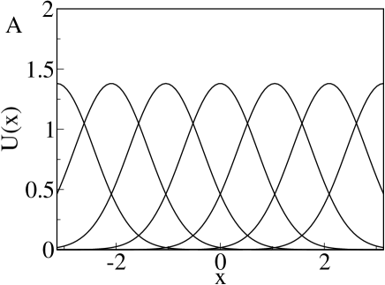
We first consider the intrinsic dynamics of the CANN model in the absence of external stimuli. It is straightforward to check that, for 0<k<kcA2ρ/(82πa)0𝑘subscript𝑘𝑐superscript𝐴2𝜌82𝜋𝑎0<k<k_{c}\equiv A^{2}\rho/(8\sqrt{2\pi}a), the network holds a continuous family of stationary states, which are (see Fig. 2A)

U~(x|z)~𝑈conditional𝑥𝑧\displaystyle\tilde{U}(x|z) =\displaystyle= U0exp[(xz)24a2],subscript𝑈0superscript𝑥𝑧24superscript𝑎2\displaystyle U_{0}\exp\left[-\frac{(x-z)^{2}}{4a^{2}}\right], (4)
r~(x|z)~𝑟conditional𝑥𝑧\displaystyle\tilde{r}(x|z) =\displaystyle= r0exp[(xz)22a2],subscript𝑟0superscript𝑥𝑧22superscript𝑎2\displaystyle r_{0}\exp\left[-\frac{(x-z)^{2}}{2a^{2}}\right], (5)

where U0=[1+(1k/kc)1/2]A/(4πak)subscript𝑈0delimited-[]1superscript1𝑘subscript𝑘𝑐12𝐴4𝜋𝑎𝑘U_{0}=[1+(1-k/k_{c})^{1/2}]A/(4\sqrt{\pi}ak) and r0=[1+(1k/kc)1/2]/(22πakρ)subscript𝑟0delimited-[]1superscript1𝑘subscript𝑘𝑐1222𝜋𝑎𝑘𝜌r_{0}=[1+(1-k/k_{c})^{1/2}]/(2\sqrt{2\pi}ak\rho). These stationary states are translationally invariant among themselves and have a Gaussian shape with a free parameter z𝑧z indicating their positions. z𝑧z is therefore the coordinate of the manifold formed by all stationary states.

The stability of the Gaussian bumps can be studied by considering the dynamics of fluctuations. Consider the network state U(x,t)=U~(x|z)+δU(x,t)𝑈𝑥𝑡~𝑈conditional𝑥𝑧𝛿𝑈𝑥𝑡U(x,t)=\tilde{U}(x|z)+\delta U(x,t). As derived in Appendix B, we have

τtδU(x,t)=𝑑xF(x,x|z)δU(x,t)δU(x,t),𝜏𝑡𝛿𝑈𝑥𝑡subscriptsuperscriptdifferential-dsuperscript𝑥𝐹𝑥conditionalsuperscript𝑥𝑧𝛿𝑈superscript𝑥𝑡𝛿𝑈𝑥𝑡\tau\frac{\partial}{\partial t}\delta U(x,t)=\int^{\infty}_{-\infty}dx^{\prime}F(x,x^{\prime}|z)\delta U(x^{\prime},t)-\delta U(x,t), (6)

where the interaction kernel F(x,x|z)𝐹𝑥conditionalsuperscript𝑥𝑧F(x,x^{\prime}|z) is given by

F(x,x|z)=2ρU(x)B[J(x,x)kρ𝑑x′′J(x,x′′)r(x′′)].𝐹𝑥conditionalsuperscript𝑥𝑧2𝜌𝑈superscript𝑥𝐵delimited-[]𝐽𝑥superscript𝑥𝑘𝜌subscriptsuperscriptdifferential-dsuperscript𝑥′′𝐽𝑥superscript𝑥′′𝑟superscript𝑥′′F(x,x^{\prime}|z)=\frac{2\rho U(x^{\prime})}{B}\left[J(x,x^{\prime})-k\rho\int^{\infty}_{-\infty}dx^{\prime\prime}J(x,x^{\prime\prime})r(x^{\prime\prime})\right]. (7)

We are interested in the eigenfunctions and eigenvalues of the kernel F(x,x|z)𝐹𝑥conditionalsuperscript𝑥𝑧F(x,x^{\prime}|z). Since the kernel is not symmetric with respect to the permutation of x𝑥x and xsuperscript𝑥x^{\prime}, we have to distinguish between its left and right eigenfunctions. To compute them, we need to choose a convenient set of basis functions. They should satisfy the boundary condition that they vanish when x𝑥x approaches ±plus-or-minus\pm\infty. A convenient choice is one that contains a basis function taking the shape of a Gaussian bump. Since the quantum ground state of the harmonic oscillator potential has a Gaussian shape, a natural choice of basis functions is the wave functions of quantum harmonic oscillators [Griffiths 2004], namely,

vn(x|z)=1(2π)1/2an!2nexp[(xz)24a2]Hn(xz2a),subscript𝑣𝑛conditional𝑥𝑧1superscript2𝜋12𝑎𝑛superscript2𝑛superscript𝑥𝑧24superscript𝑎2subscript𝐻𝑛𝑥𝑧2𝑎v_{n}(x|z)=\frac{1}{\sqrt{(2\pi)^{1/2}an!2^{n}}}\exp\left[-\frac{(x-z)^{2}}{4a^{2}}\right]H_{n}\left(\frac{x-z}{\sqrt{2}a}\right), (8)

where Hnsubscript𝐻𝑛H_{n} are the n𝑛nth-order Hermite polynomials for n=0,1,2,𝑛012n=0,1,2,\ldots, which can be expressed as the derivatives of the Gaussian function [Griffiths 2004]

vn(x|z)=(1)n(2a)n1/2π1/2n!2nexp[(xz)24a2](ddx)nexp[(xz)22a2].subscript𝑣𝑛conditional𝑥𝑧superscript1𝑛superscript2𝑎𝑛12superscript𝜋12𝑛superscript2𝑛superscript𝑥𝑧24superscript𝑎2superscript𝑑𝑑𝑥𝑛superscript𝑥𝑧22superscript𝑎2v_{n}(x|z)={\frac{(-1)^{n}(\sqrt{2}a)^{n-1/2}}{\sqrt{\pi^{1/2}n!2^{n}}}}\exp\left[{\frac{(x-z)^{2}}{4a^{2}}}\right]\left(\frac{d}{dx}\right)^{n}\exp\left[-{\frac{(x-z)^{2}}{2a^{2}}}\right]. (9)

This choice of basis functions has the further advantage that an abundance of mathematical properties are available for our analysis, as summarized in Appendix A.

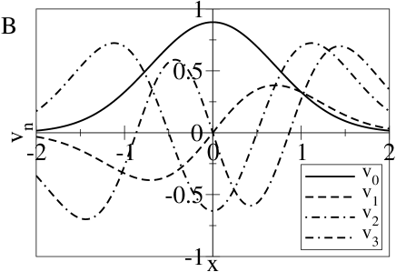
Fig. 2B pictures the first four wave functions. We see that:

  • The ground state of the quantum harmonic oscillator,

    v0(x|z)=U~(x|z)U0(2π)1/2a,subscript𝑣0conditional𝑥𝑧~𝑈conditional𝑥𝑧subscript𝑈0superscript2𝜋12𝑎v_{0}(x|z)=\frac{\tilde{U}(x|z)}{U_{0}\sqrt{(2\pi)^{1/2}a}}, (10)

    corresponds to the stationary state of the network.

  • The first excited state of the quantum harmonic oscillator,

    v1(x|z)=2aU0(2π)1/2aU~(x|z)z,subscript𝑣1conditional𝑥𝑧2𝑎subscript𝑈0superscript2𝜋12𝑎~𝑈conditional𝑥𝑧𝑧v_{1}(x|z)=\frac{2a}{U_{0}\sqrt{(2\pi)^{1/2}a}}\frac{\partial\tilde{U}(x|z)}{\partial z}, (11)

    corresponds to the positional shift of the stationary state.

  • The second and third excited states, v2(x|z)subscript𝑣2conditional𝑥𝑧v_{2}(x|z) and v3(x|z)subscript𝑣3conditional𝑥𝑧v_{3}(x|z), respectively correspond to the distortions in the width and skewness of the bump.

Refer to caption
Refer to caption
Figure 2: (A) The Gaussian-shaped stationary states of the network. (B) The first four basis functions of the quantum harmonic oscillators, representing distortions in the height, position, width and skewness of the Gaussian bump.

To express δU(x,t)𝛿𝑈𝑥𝑡\delta U(x,t) in terms of the eigenfunctions vn(x|z)subscript𝑣𝑛conditional𝑥𝑧v_{n}(x|z) using Eq. (6), we consider F(x,x|z)𝐹𝑥conditionalsuperscript𝑥𝑧F(x,x^{\prime}|z) as an operator acting on vn(x|z)subscript𝑣𝑛conditional𝑥𝑧v_{n}(x|z). Since vn(x|z)subscript𝑣𝑛conditional𝑥𝑧v_{n}(x|z) is a basis, we have

𝑑xF(x,x|z)vn(x|z)=mvm(x|z)Fmn,subscriptsuperscriptdifferential-dsuperscript𝑥𝐹𝑥conditionalsuperscript𝑥𝑧subscript𝑣𝑛conditionalsuperscript𝑥𝑧subscript𝑚subscript𝑣𝑚conditional𝑥𝑧subscript𝐹𝑚𝑛\int^{\infty}_{-\infty}dx^{\prime}F(x,x^{\prime}|z)v_{n}(x^{\prime}|z)=\sum_{m}v_{m}(x|z)F_{mn}, (12)

where Fmnsubscript𝐹𝑚𝑛F_{mn} is the representation of the kernel F(x,x|z)𝐹𝑥conditionalsuperscript𝑥𝑧F(x,x^{\prime}|z) in the basis vn(x|z)subscript𝑣𝑛conditional𝑥𝑧v_{n}(x|z), given by

Fmn=𝑑x𝑑xvm(x|z)F(x,x|z)vn(x|z).subscript𝐹𝑚𝑛subscriptsuperscriptdifferential-d𝑥subscriptsuperscriptdifferential-dsuperscript𝑥subscript𝑣𝑚conditional𝑥𝑧𝐹𝑥conditionalsuperscript𝑥𝑧subscript𝑣𝑛conditionalsuperscript𝑥𝑧F_{mn}=\int^{\infty}_{-\infty}dx\int^{\infty}_{-\infty}dx^{\prime}v_{m}(x|z)F(x,x^{\prime}|z)v_{n}(x^{\prime}|z). (13)

As derived in Appendix B for the particular choice of the output function (1) and the neural interactions (3), the elements of the matrix Fmnsubscript𝐹𝑚𝑛F_{mn} are given by

Fmn={11k/kc,m=n=0;21nn!m!(1)nm22nm2(nm2)!,nm being an even integer;0,otherwise.subscript𝐹𝑚𝑛cases11𝑘subscript𝑘𝑐𝑚𝑛0superscript21𝑛𝑛𝑚superscript1𝑛𝑚2superscript2𝑛𝑚2𝑛𝑚2nm being an even integer0otherwiseF_{mn}=\left\{\begin{array}[]{ll}1-\sqrt{1-k/k_{c}},&m=n=0;\\ 2^{1-n}\sqrt{\frac{n!}{m!}}\frac{(-1)^{\frac{n-m}{2}}}{2^{\frac{n-m}{2}}\displaystyle\left(\frac{n-m}{2}\right)!},&\mbox{$n-m$ being an even integer};\\ 0,&\mbox{otherwise}.\end{array}\right. (14)

By using the matrix Fmnsubscript𝐹𝑚𝑛F_{mn}, we can calculate the eigenvalues and the first four right eigenfunctions of the kernel F(x,x|z)𝐹𝑥conditionalsuperscript𝑥𝑧F(x,x^{\prime}|z), which are (see Appendix B)

λ0subscript𝜆0\displaystyle\lambda_{0} =\displaystyle= 11k/kc,11𝑘subscript𝑘𝑐\displaystyle 1-\sqrt{1-k/k_{c}}, (15)
λnsubscript𝜆𝑛\displaystyle\lambda_{n} =\displaystyle= 21n,forn1,,formulae-sequencesuperscript21𝑛for𝑛1\displaystyle 2^{1-n},~{}~{}~{}~{}\mbox{for}~{}~{}n\geq 1,\ldots, (16)
u0R(x|z)subscriptsuperscript𝑢𝑅0conditional𝑥𝑧\displaystyle u^{R}_{0}(x|z) =\displaystyle= v0(x|z),subscript𝑣0conditional𝑥𝑧\displaystyle v_{0}(x|z), (17)
u1R(x|z)subscriptsuperscript𝑢𝑅1conditional𝑥𝑧\displaystyle u^{R}_{1}(x|z) =\displaystyle= v1(x|z),subscript𝑣1conditional𝑥𝑧\displaystyle v_{1}(x|z), (18)
u2R(x|z)subscriptsuperscript𝑢𝑅2conditional𝑥𝑧\displaystyle u^{R}_{2}(x|z) =\displaystyle= 1/2D0v0(x|z)+121k/kcD0v2(x|z),12subscript𝐷0subscript𝑣0conditional𝑥𝑧121𝑘subscript𝑘𝑐subscript𝐷0subscript𝑣2conditional𝑥𝑧\displaystyle{\frac{\sqrt{1/2}}{D_{0}}}v_{0}(x|z)+\frac{1-2\sqrt{1-k/k_{c}}}{D_{0}}v_{2}(x|z), (19)
u3R(x|z)subscriptsuperscript𝑢𝑅3conditional𝑥𝑧\displaystyle u^{R}_{3}(x|z) =\displaystyle= 17v1(x,z)+67v3(x,z),17subscript𝑣1𝑥𝑧67subscript𝑣3𝑥𝑧\displaystyle\sqrt{\frac{1}{7}}v_{1}(x,z)+\sqrt{\frac{6}{7}}v_{3}(x,z), (20)

where

D0=[(121k/kc)2+1/2]1/2.subscript𝐷0superscriptdelimited-[]superscript121𝑘subscript𝑘𝑐21212D_{0}=\left[\left(1-2\sqrt{1-k/k_{c}}\right)^{2}+1/2\right]^{1/2}. (21)

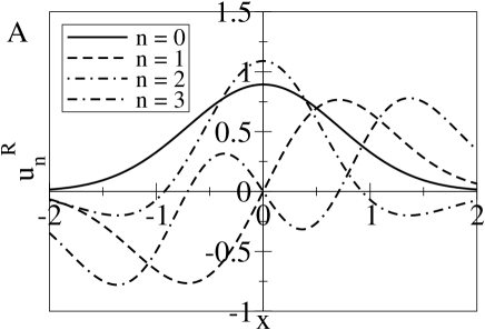
We note that u1R(x|z)=v1(x|z)subscriptsuperscript𝑢𝑅1conditional𝑥𝑧subscript𝑣1conditional𝑥𝑧u^{R}_{1}(x|z)=v_{1}(x|z) and λ1=1subscript𝜆11\lambda_{1}=1. Fig. 3A illustrates the first four right eigenfunctions of F𝐹F.

The right eigenfunctions of F𝐹F correspond to the various distortion modes of the bump. For example, u0R(x|z)subscriptsuperscript𝑢𝑅0conditional𝑥𝑧u^{R}_{0}(x|z) corresponds to the amplitude distortion of the bump, and u1R(x|z)subscriptsuperscript𝑢𝑅1conditional𝑥𝑧u^{R}_{1}(x|z) to the positional shift. Starting from n=3𝑛3n=3, unR(x|z)subscriptsuperscript𝑢𝑅𝑛conditional𝑥𝑧u^{R}_{n}(x|z) are linear combinations of vk(x|z)subscript𝑣𝑘conditional𝑥𝑧v_{k}(x|z), where k=n,n2,𝑘𝑛𝑛2k=n,n-2,\ldots. Some of them may be dominated by a specific type of distortion, such as u3Rsubscriptsuperscript𝑢𝑅3u^{R}_{3} in Eq. (20) being dominated by the skewness. However, generally speaking, various distortion features have been coupled in the eigenfunctions of the interaction kernel. To avoid confusion, we continue to use vn(x|z)subscript𝑣𝑛conditional𝑥𝑧v_{n}(x|z) as our basis functions in the rest of the paper.

To identify the contributions of unR(x|z)subscriptsuperscript𝑢𝑅𝑛conditional𝑥𝑧u^{R}_{n}(x|z) to the network dynamics, we express δU(x,t)𝛿𝑈𝑥𝑡\delta U(x,t) in (6) as a linear combination of unR(x|z)subscriptsuperscript𝑢𝑅𝑛conditional𝑥𝑧u^{R}_{n}(x|z), namely, δU(x,t)=nδUn(z,t)unR(x|z)𝛿𝑈𝑥𝑡subscript𝑛𝛿subscript𝑈𝑛𝑧𝑡subscriptsuperscript𝑢𝑅𝑛conditional𝑥𝑧\delta U(x,t)=\sum_{n}\delta U_{n}(z,t)u^{R}_{n}(x|z). Using the orthonormality of the left and right eigenfunctions of F(x,x|z)𝐹𝑥conditionalsuperscript𝑥𝑧F(x,x^{\prime}|z), we have

δUn(z,t)=𝑑xδU(x,t)unL(x|z).𝛿subscript𝑈𝑛𝑧𝑡subscriptsuperscriptdifferential-d𝑥𝛿𝑈𝑥𝑡subscriptsuperscript𝑢𝐿𝑛conditional𝑥𝑧\delta U_{n}(z,t)=\int^{\infty}_{-\infty}dx\delta U(x,t)u^{L}_{n}(x|z). (22)

Assume that the motion of the bump is slow, so that dz/dt𝑑𝑧𝑑𝑡dz/dt becomes negligible in Eq. (6); as we shall see, this assumption is valid as long as the external stimulus is sufficiently weak. Then, the projection of Eq. (6) on the eigenfunctions become

τddtδUn(z,t)=(λn1)δUn(z,t).𝜏𝑑𝑑𝑡𝛿subscript𝑈𝑛𝑧𝑡subscript𝜆𝑛1𝛿subscript𝑈𝑛𝑧𝑡\tau\frac{d}{dt}\delta U_{n}(z,t)=(\lambda_{n}-1)\delta U_{n}(z,t). (23)

Hence,

δUn(z,t)=δUn(z,0)exp[(1λn)tτ],𝛿subscript𝑈𝑛𝑧𝑡𝛿subscript𝑈𝑛𝑧01subscript𝜆𝑛𝑡𝜏\delta U_{n}(z,t)=\delta U_{n}(z,0)\exp\left[-{\frac{(1-\lambda_{n})t}{\tau}}\right], (24)

where δUn(z,0)𝛿subscript𝑈𝑛𝑧0\delta U_{n}(z,0) is the initial value of the projection.

Eq. (24) tells us that, since λ1=1subscript𝜆11\lambda_{1}=1, the bump distortion δU1𝛿subscript𝑈1\delta U_{1}, which corresponds to the positional shift of the bump, is sustained under the network dynamics. This is the mathematical expression of the neutral stability of the stationary states of the network. The eigenvalues for all other eigenfunctions are all less than one. Since these other modes of bump distortions decay exponentially with the time constant τ/(1λn)𝜏1subscript𝜆𝑛\tau/(1-\lambda_{n}), their contributions on the network dynamics are small when compared with that due to the positional shift. An intuitive illustration of the decomposition of the network dynamics is given in Fig. 3B.

Refer to caption
Refer to caption
Figure 3: (A) The first four right eigenfunctions of the interaction kernel F(x,x|z)𝐹𝑥conditionalsuperscript𝑥𝑧F(x,x^{\prime}|z) with k/kc=1/2𝑘subscript𝑘𝑐12k/k_{c}=1/2. (B) The distortions of the network state are decomposed into three parts, namely, distortions in the height, position and all other shapes.

The fact that the dynamics of a CANN is dominated by only a few motion modes suggests that we may use this property to simplify the description of the network dynamics; that is, we can project the network dynamics onto its dominating modes. By this, we can analytically quantify the tracking bahviors of a CANN.

The Landscape of the State Space

It is instructive to illustrate the energy landscape in the state space of a CANN. In the dynamical system that we are studying, we do not have a Lyapunov function. This is evident from the fact that the interaction matrix Fmnsubscript𝐹𝑚𝑛F_{mn} is not symmetric. Nevertheless, at each peak position z𝑧z, one can define an effective energy function E(z)=n(1λn)[δUn(z)]2/2𝐸𝑧subscript𝑛1subscript𝜆𝑛superscriptdelimited-[]𝛿subscript𝑈𝑛𝑧22E(z)=\sum_{n}(1-\lambda_{n})[\delta U_{n}(z)]^{2}/2, with δUn(z)𝛿subscript𝑈𝑛𝑧\delta U_{n}(z) being the projection of U(x)U~(x|z)𝑈𝑥~𝑈conditional𝑥𝑧U(x)-\tilde{U}(x|z) on the eigenfunction un(x|z)subscript𝑢𝑛conditional𝑥𝑧u_{n}(x|z). Then, the dynamics in Eq. (6) or (23) can be locally described by the gradient descent of E(z)𝐸𝑧E(z) in the space of δUn(z)𝛿subscript𝑈𝑛𝑧\delta U_{n}(z). E(z)𝐸𝑧E(z) has the minimum value of zero when δUn(z)=0𝛿subscript𝑈𝑛𝑧0\delta U_{n}(z)=0 for n1𝑛1n\neq 1 and δU1(z)𝛿subscript𝑈1𝑧\delta U_{1}(z) can take any value since λ1=1subscript𝜆11\lambda_{1}=1. This corresponds to the picture that the bump’s position shifts, but the shape of the bump remains unchanged. When z𝑧z varies, the solution of E(z)=0𝐸𝑧0E(z)=0 traces a curve in the state space, facilitating the local gradient descent dynamics of the network, with the tangent of the curve at each point defining the direction of neutral stability. We can envisage this by a canyon surrounding the curve as shown in Fig. 1, and a small force along the tangent of the canyon can move the network state easily.

The External Input

To proceed, we need to define the external input. Without loss of generality, we choose

Iext(x,t)=αU0exp[(xz0)24a2]+ση(x,t),subscript𝐼ext𝑥𝑡𝛼subscript𝑈0superscript𝑥subscript𝑧024superscript𝑎2𝜎𝜂𝑥𝑡I_{\rm ext}(x,t)=\alpha U_{0}\exp\left[-{\frac{(x-z_{0})^{2}}{4a^{2}}}\right]+\sigma\eta(x,t), (25)

where α𝛼\alpha and σ𝜎\sigma indicate the strength of the signal and the noise, respectively. η(x,t)𝜂𝑥𝑡\eta(x,t) is Gaussian white noise, satisfying η(x,t)=0delimited-⟨⟩𝜂𝑥𝑡0\langle\eta(x,t)\rangle=0 and η(x,t)η(x,t)=δ(xx)δ(tt)delimited-⟨⟩𝜂𝑥𝑡𝜂superscript𝑥superscript𝑡𝛿𝑥superscript𝑥𝛿𝑡superscript𝑡\langle\eta(x,t)\eta(x^{\prime},t^{\prime})\rangle=\delta(x-x^{\prime})\delta(t-t^{\prime}). The signal term has the effect of driving the bump to the stimulus location z0subscript𝑧0z_{0}, and the noise term tends to shift the bump position randomly. Our results are qualitatively independent of the exact form of the external input. We may choose other forms for the external input. The main conclusions will be the same once the chosen external input has a unimodal shape and has the effect of driving the bump to the stimulus position.

The Setting of the Simulation Experiments

We will use simulation experiments to confirm the theoretical analysis. Here, we describe the setting of simulation experiments to be used below. The network consists of N𝑁N neurons. Their preferred stimuli x𝑥x are evenly distributed in the range (π,π]𝜋𝜋(-\pi,\pi] and satisfy the periodic condition, namely, U(x,t)=U(x+2π,t)𝑈𝑥𝑡𝑈𝑥2𝜋𝑡U(x,t)=U(x+2\pi,t). In the simulation, the integration in the continuum limit is changed to the summation accordingly, i.e., ρ𝑑xi=1N𝜌differential-d𝑥superscriptsubscript𝑖1𝑁\rho\int dx\to\sum_{i=1}^{N}. We choose a=0.52π𝑎0.5much-less-than2𝜋a=0.5\ll 2\pi, so that comparison with the theoretical analysis for x(,)𝑥x\in(-\infty,\infty) holds.

3 Tracking Dynamics in the Weak Input Limit

We consider first the case when the external input is sufficiently small, i.e., α1much-less-than𝛼1\alpha\ll 1 and σ1much-less-than𝜎1\sigma\ll 1. In this case, we can reasonably assume that the network dynamics is dominated by the positional shift of the bump, and we can thus ignore other motion modes, that is, U(x,t)U~(x|z(t))𝑈𝑥𝑡~𝑈conditional𝑥𝑧𝑡U(x,t)\approx\tilde{U}(x|z(t)), with only the bump position z(t)𝑧𝑡z(t) varying with time. As will be shown in Section 4, this actually corresponds to n=0𝑛0n=0 perturbation in the general perturbative method.

After projecting the network dynamics, Eq. (2), on the basis functions v1(x|z(t))subscript𝑣1conditional𝑥𝑧𝑡v_{1}(x|z(t)), we obtain (see Appendix C)

dzdt=ατ(zz0)exp[(zz0)28a2]+2Dη1(t),𝑑𝑧𝑑𝑡𝛼𝜏𝑧subscript𝑧0superscript𝑧subscript𝑧028superscript𝑎22𝐷subscript𝜂1𝑡\frac{dz}{dt}=-\frac{\alpha}{\tau}(z-z_{0})\exp\left[-\frac{(z-z_{0})^{2}}{8a^{2}}\right]+\sqrt{2D}\eta_{1}(t), (26)

where D=2aσ2/(U02τ2π)𝐷2𝑎superscript𝜎2superscriptsubscript𝑈02superscript𝜏2𝜋D=\sqrt{2}a\sigma^{2}/(U_{0}^{2}\tau^{2}\sqrt{\pi}) is the diffusion constant, and η1(t)subscript𝜂1𝑡\eta_{1}(t) is the overlap of η(x,t)𝜂𝑥𝑡\eta(x,t) with v1(x|z(t))subscript𝑣1conditional𝑥𝑧𝑡v_{1}(x|z(t)) given by

η1(t)=𝑑xη(x,t)v1(x|z(t)),subscript𝜂1𝑡subscriptsuperscriptdifferential-d𝑥𝜂𝑥𝑡subscript𝑣1conditional𝑥𝑧𝑡\eta_{1}(t)=\int^{\infty}_{-\infty}dx\eta(x,t)v_{1}(x|z(t)), (27)

which satisfies

η1(t)=0andη1(t)η1(t)=δ(tt).formulae-sequencedelimited-⟨⟩subscript𝜂1𝑡0anddelimited-⟨⟩subscript𝜂1𝑡subscript𝜂1superscript𝑡𝛿𝑡superscript𝑡\langle\eta_{1}(t)\rangle=0\quad{\rm and}\quad\langle\eta_{1}(t)\eta_{1}(t^{\prime})\rangle=\delta(t-t^{\prime}). (28)

This equation represents a one-dimensional Ornstein-Uhlenbeck process for the motion of the bump position in the state space [Tuckwell 1988]. Its meaning is straightforward: the first term on the right-hand side of the equation represents the contribution of the stimulus, whose effect is to pull the bump to the stimulus position z0subscript𝑧0z_{0}; the second term represents noise, which tends to shift the bump position randomly. This equation agrees with Eq. (3.7) in [Wu, Hamaguchi, and Amari 2008], which considers |zz0|amuch-less-than𝑧subscript𝑧0𝑎|z-z_{0}|\ll a and hence e(zz0)2/8a21superscript𝑒superscript𝑧subscript𝑧028superscript𝑎21e^{-(z-z_{0})^{2}/8a^{2}}\approx 1.

The distribution of the bump position can be calculated. The pull term in Eq. (26) can be written as the gradient of a potential,

V(z)=4a2ατexp[(zz0)28a2],𝑉𝑧4superscript𝑎2𝛼𝜏superscript𝑧subscript𝑧028superscript𝑎2V(z)=-\frac{4a^{2}\alpha}{\tau}\exp\left[-\frac{(z-z_{0})^{2}}{8a^{2}}\right], (29)

so that Eq. (26) can be written as a Langevin equation,

dzdt=Vz+2Dη(t).𝑑𝑧𝑑𝑡𝑉𝑧2𝐷𝜂𝑡\frac{dz}{dt}=-\frac{\partial V}{\partial z}+\sqrt{2D}\eta(t). (30)

This implies that z𝑧z satisfies a Boltzmann distribution [Ma 1976],

P(z)exp[V(z)D].similar-to𝑃𝑧𝑉𝑧𝐷P(z)\sim\exp\left[-\frac{V(z)}{D}\right]. (31)

Since the pull is maximum at z=z0±2a𝑧plus-or-minussubscript𝑧02𝑎z=z_{0}\pm 2a, two noise regimes can be identified. In the low noise regime, where (zz0)24a2much-less-thandelimited-⟨⟩superscript𝑧subscript𝑧024superscript𝑎2\langle(z-z_{0})^{2}\rangle\ll 4a^{2}, the bump position is effectively trapped in a parabolic potential, whereas in the high noise regime with (zz0)24a2much-greater-thandelimited-⟨⟩superscript𝑧subscript𝑧024superscript𝑎2\langle(z-z_{0})^{2}\rangle\gg 4a^{2}, the pull vanishes and the motion of the bump resembles a random walk with [z(t)z0]2=2Dtdelimited-⟨⟩superscriptdelimited-[]𝑧𝑡subscript𝑧022𝐷𝑡\langle[z(t)-z_{0}]^{2}\rangle=2Dt loosely coupled to the stimulus.

However, simulation results show that Eq. (31) underestimates the variance of the bump position. This is because we have considered only the overlap of η(x,t)𝜂𝑥𝑡\eta(x,t) with v1(x|z(t))subscript𝑣1conditional𝑥𝑧𝑡v_{1}(x|z(t)). As will be shown in the perturbative approach, overlaps with other components cannot be neglected.

By using the simplified dynamics in Eq. (26), we explore two tracking behavior of the network, namely, the tracking of a moving stimulus and the catching up of an abrupt change in the stimulus.

3.1 The Condition for Successful Tracking

Suppose that the stimulus is moving at a constant velocity v𝑣v and the noise is low and negligible. The dynamical equation becomes identical to Eq. (26) after the transients, with z0subscript𝑧0z_{0} replaced by vt𝑣𝑡vt. Denoting the lag of the bump behind the stimulus as s=z0z𝑠subscript𝑧0𝑧s=z_{0}-z, we have

dsdt𝑑𝑠𝑑𝑡\displaystyle{\frac{ds}{dt}} =\displaystyle= dz0dtdzdt𝑑subscript𝑧0𝑑𝑡𝑑𝑧𝑑𝑡\displaystyle{\frac{dz_{0}}{dt}}-{\frac{dz}{dt}} (32)
=\displaystyle= vαsτexp[s28a2]𝑣𝛼𝑠𝜏superscript𝑠28superscript𝑎2\displaystyle v-\frac{\alpha s}{\tau}\exp\left[-\frac{s^{2}}{8a^{2}}\right]
=\displaystyle= vg(s).𝑣𝑔𝑠\displaystyle v-g(s).

The size of the lag s𝑠s is determined by two competing factors: the first term represents the movement of the stimulus, which tends to enlarge the lag; and the second term represents the collective effects of the neuronal recurrent interactions, which tends to shorten the lag. The tracking is achieved when these two forces match each other, i.e., v=g(s)𝑣𝑔𝑠v=g(s); otherwise, s𝑠s diverges.

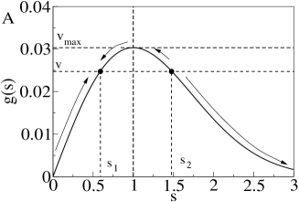
Fig. 4A shows that the function g(s)𝑔𝑠g(s) is concave and has the maximum value of gmax=2αa/(τe)subscript𝑔max2𝛼𝑎𝜏𝑒g_{\rm max}=2\alpha a/(\tau\sqrt{e}) at s=2a𝑠2𝑎s=2a. This means that if v>gmax𝑣subscript𝑔maxv>g_{\rm max}, the network is unable to track the stimulus. Thus, gmaxsubscript𝑔maxg_{\rm max} defines the maximum trackable speed of a moving stimulus to the network. Notably, gmaxsubscript𝑔maxg_{\rm max} increases with the strength of the external signal α𝛼\alpha and the range of neuronal recurrent interactions a𝑎a. This is reasonable since it is the neuronal interactions that induce the movement of the bump. gmaxsubscript𝑔maxg_{\rm max} decreases with the time constant of the network τ𝜏\tau, as this reflects the responsiveness of the network to external inputs.

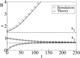
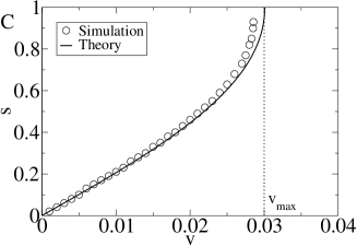
On the other hand, for v<gmax𝑣subscript𝑔maxv<g_{\rm max}, there is a stable and unstable fixed point, denoted as s1subscript𝑠1s_{1} and s2subscript𝑠2s_{2} respectively, in Fig. 4A. When the initial lag is less than s2subscript𝑠2s_{2}, it will converge to s1subscript𝑠1s_{1}. Otherwise, the tracking of the stimulus will be lost. Intuitively, this means that the propagation of neuronal activities in the network needs to be quick enough to compensate for the initial lag behind the stimulus. Figs. 4B and 4C show that the analytical results of Eq. (32) agree well with the simulation results.
Refer to caption
Refer to caption
Refer to caption
Figure 4: (A) The function g(s)𝑔𝑠g(s) and the stable and unstable fixed points of Eq. (32). (B) The time dependence of the separation s𝑠s starting from different initial values. v=0.025𝑣0.025v=0.025. (C) The dependence of the terminal separation s𝑠s on the speed v𝑣v. Parameters: N=200𝑁200N=200, k=0.5𝑘0.5k=0.5, a=0.5𝑎0.5a=0.5, τ=1𝜏1\tau=1, A=2πa𝐴2𝜋𝑎A=\sqrt{2\pi}a, ρ=N/2π𝜌𝑁2𝜋\rho=N/2\pi and α=0.05𝛼0.05\alpha=0.05.

3.2 The Reaction Time

Another tracking behavior we study is the response to a stimulus experiencing an abrupt change. We measure how long it takes for the network to catch up with this change, i.e., the reaction time. Suppose that the network has reached a steady state at t<0𝑡0t<0, and the stimulus position jumps from 00 to z0subscript𝑧0z_{0} suddenly at t=0𝑡0t=0. This is the typical setting in experiments studying mental rotation behavior [Georgopoulos, Taira, and Lukashin 1993, Ben-Yishai, Lev Bar-Or, and Sompolinsky 1995, Wu and Amari 2005]. The reaction time can be obtained by integrating Eq. (26) with the initial value z(t=0)=0𝑧𝑡00z(t=0)=0.

When the noise is low and the jump size |z0|subscript𝑧0|z_{0}| is much smaller than the range a𝑎a of neuronal interactions, we can derive an analytical expression for the reaction time. In this case, Eq. (26) is approximated as

τdzdtα(z0z).𝜏𝑑𝑧𝑑𝑡𝛼subscript𝑧0𝑧\tau{\frac{dz}{dt}}\approx\alpha(z_{0}-z). (33)

We define the reaction time T𝑇T as the time it takes for the bump to move to a small threshold distance θ𝜃\theta from the stimulus. T𝑇T is calculated to be

Tταln(|z0|θ).𝑇𝜏𝛼subscript𝑧0𝜃T\approx{\frac{\tau}{\alpha}}\ln\left({\frac{|z_{0}|}{\theta}}\right). (34)

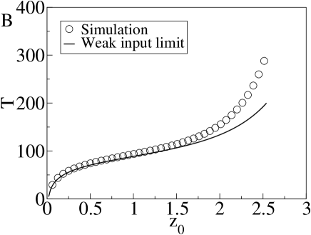
This reveals that with small jump sizes, the reaction time of a CANN increases logarithmically with the jump size.

Fig. 5 compares the simulation results with our theoretical predictions based on Eq. (26). We see that with small jump sizes, they agree very well with each other, and the reaction time indeed has a logarithmic nature in its increase with the jump size. However, we also notice that with large jump sizes, there is considerable discrepancy between the simulation results and the theoretical predictions. This is because we have only considered the positional shift in the network dynamics. To improve the results, more motion modes must be included.
Refer to caption
Refer to caption
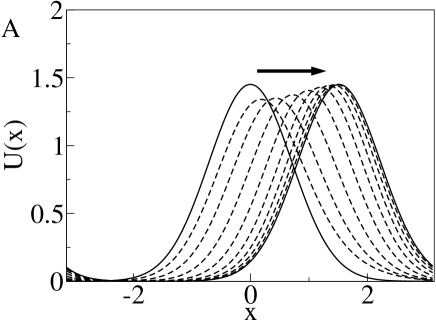
Figure 5: (A) The tracking process of the network. (B) The reaction time vs. the jump size |z0|subscript𝑧0|z_{0}|. Parameters: θ=π/200𝜃𝜋200\theta=\pi/200 and the rest are the same as Fig. 4.

4 Tracking Dynamics: A Comprehensive Study

In this section, we develop a time-dependent perturbation approach to systematically improve the description of the network dynamics. Since the network dynamics is primarily dominated by the positional shift of the bump, with high-order distortions from other motion modes, we consider the network states with the following form,

U(x,t)=U~(x|z(t))+n=0an(t)vn(x|z(t)),𝑈𝑥𝑡~𝑈conditional𝑥𝑧𝑡superscriptsubscript𝑛0subscript𝑎𝑛𝑡subscript𝑣𝑛conditional𝑥𝑧𝑡U(x,t)=\tilde{U}(x|z(t))+\sum_{n=0}^{\infty}a_{n}(t)v_{n}(x|z(t)), (35)

where the bump position z(t)𝑧𝑡z(t) and the coefficients {an(t)}subscript𝑎𝑛𝑡\{a_{n}(t)\} specify the network state.

The external input can be similarly expressed as

Iext(x,t)=n=0In(t)vn(x|z),subscript𝐼ext𝑥𝑡superscriptsubscript𝑛0subscript𝐼𝑛𝑡subscript𝑣𝑛conditional𝑥𝑧I_{\rm ext}(x,t)=\sum_{n=0}^{\infty}I_{n}(t)v_{n}(x|z), (36)

with In=𝑑xIext(x,t)vn(x|z)subscript𝐼𝑛differential-d𝑥subscript𝐼ext𝑥𝑡subscript𝑣𝑛conditional𝑥𝑧I_{n}=\int dxI_{\rm ext}(x,t)v_{n}(x|z).

By substituting Eqs. (35) and (36) into Eq. (2), and making use of the orthonormality and completeness of vn(x|z)subscript𝑣𝑛conditional𝑥𝑧v_{n}(x|z), we obtain the perturbative equation for an(t)subscript𝑎𝑛𝑡a_{n}(t) as (see Appendix D)

(ddt+1λnτ)an𝑑𝑑𝑡1subscript𝜆𝑛𝜏subscript𝑎𝑛\displaystyle\left(\frac{d}{dt}+\frac{1-\lambda_{n}}{\tau}\right)a_{n} =\displaystyle= Inτ[U0(2π)1/2aδn1+nan1n+1an+1]12adzdtsubscript𝐼𝑛𝜏delimited-[]subscript𝑈0superscript2𝜋12𝑎subscript𝛿𝑛1𝑛subscript𝑎𝑛1𝑛1subscript𝑎𝑛112𝑎𝑑𝑧𝑑𝑡\displaystyle\frac{I_{n}}{\tau}-\left[U_{0}\sqrt{(2\pi)^{1/2}a}\delta_{n1}+\sqrt{n}a_{n-1}-\sqrt{n+1}a_{n+1}\right]\frac{1}{2a}\frac{dz}{dt} (37)
+\displaystyle+ 1τr=1(n+2r)!n!(1)r2n+3r1r!an+2r.1𝜏superscriptsubscript𝑟1𝑛2𝑟𝑛superscript1𝑟superscript2𝑛3𝑟1𝑟subscript𝑎𝑛2𝑟\displaystyle\frac{1}{\tau}\sum_{r=1}^{\infty}\sqrt{\frac{(n+2r)!}{n!}}\frac{(-1)^{r}}{2^{n+3r-1}r!}a_{n+2r}.

The center-of-mass position z(t)𝑧𝑡z(t) is determined from the self-consistent condition,

z(t)=𝑑xU(x,t)x𝑑xU(x,t).𝑧𝑡superscriptsubscriptdifferential-d𝑥𝑈𝑥𝑡𝑥superscriptsubscriptdifferential-d𝑥𝑈𝑥𝑡z(t)=\frac{\int_{-\infty}^{\infty}dxU(x,t)x}{\int_{-\infty}^{\infty}dxU(x,t)}. (38)

By combining Eqs.(37) and (38) and denoting the product of the positive integers n,n2,𝑛𝑛2n,n-2,\ldots as n!!double-factorial𝑛n!!, we obtain an equation for the bump velocity (see Appendix D),

dzdt=2aτI1+n=3,oddn!!(n1)!!In+a1U0(2π)1/2a+n=0,even(n1)!!n!!an.𝑑𝑧𝑑𝑡2𝑎𝜏subscript𝐼1superscriptsubscript𝑛3odddouble-factorial𝑛double-factorial𝑛1subscript𝐼𝑛subscript𝑎1subscript𝑈0superscript2𝜋12𝑎superscriptsubscript𝑛0evendouble-factorial𝑛1double-factorial𝑛subscript𝑎𝑛\frac{dz}{dt}=\frac{2a}{\tau}\frac{I_{1}+\sum_{n=3,\rm odd}^{\infty}\sqrt{\frac{n!!}{(n-1)!!}}I_{n}+a_{1}}{U_{0}\sqrt{(2\pi)^{1/2}a}+\sum_{n=0,\rm even}^{\infty}\sqrt{\frac{(n-1)!!}{n!!}}a_{n}}. (39)

Eqs. (37) and (39) are the master equations of the perturbative method. For the perturbation order specified by n𝑛n, we include the coefficients from a0subscript𝑎0a_{0} up to ansubscript𝑎𝑛a_{n}, and the input components from I0subscript𝐼0I_{0} up to Insubscript𝐼𝑛I_{n}, and at least I1subscript𝐼1I_{1}, which is the lowest order of input that drives the dynamics. By choosing different orders of perturbation, we can approximate the network dynamics to different accuracies.

The components of the external input in vn(x|z)subscript𝑣𝑛conditional𝑥𝑧v_{n}(x|z) are calculated to be (see Appendix E)

In(t)=αU0exp[(z0z)28a2](z0z2a)n(2π)1/2an!+σηn(t),subscript𝐼𝑛𝑡𝛼subscript𝑈0superscriptsubscript𝑧0𝑧28superscript𝑎2superscriptsubscript𝑧0𝑧2𝑎𝑛superscript2𝜋12𝑎𝑛𝜎subscript𝜂𝑛𝑡I_{n}(t)=\alpha U_{0}\exp\left[-\frac{(z_{0}-z)^{2}}{8a^{2}}\right]\left(\frac{z_{0}-z}{2a}\right)^{n}\sqrt{\frac{(2\pi)^{1/2}a}{n!}}+\sigma\eta_{n}(t), (40)

where the noise term ηn(t)subscript𝜂𝑛𝑡\eta_{n}(t) satisfies ηn(t)=0delimited-⟨⟩subscript𝜂𝑛𝑡0\langle\eta_{n}(t)\rangle=0 and ηm(t)ηn(t)=δmnδ(tt)delimited-⟨⟩subscript𝜂𝑚𝑡subscript𝜂𝑛superscript𝑡subscript𝛿𝑚𝑛𝛿𝑡superscript𝑡\langle\eta_{m}(t)\eta_{n}(t^{\prime})\rangle=\delta_{mn}\delta(t-t^{\prime}).

4.1 The Weak Input Limit

We first compare the perturbative approach with the weak input limit by ignoring all distortion modes of the bump; that is, we set an=0subscript𝑎𝑛0a_{n}=0 for all n𝑛n. Due to the readiness of the bump to shift its position, the lowest order of the external stimulus to be included is I1subscript𝐼1I_{1} according to Eq. (39). Thus, in the n=0𝑛0n=0 perturbation, Eq. (39) becomes

dzdt=2aτI1U0(2π)1/2a.𝑑𝑧𝑑𝑡2𝑎𝜏subscript𝐼1subscript𝑈0superscript2𝜋12𝑎\frac{dz}{dt}=\frac{2a}{\tau}\frac{I_{1}}{U_{0}\sqrt{(2\pi)^{1/2}a}}. (41)

After substituting I1subscript𝐼1I_{1} from Eq. (40) into Eq. (41), we obtain Eq. (26), which is equivalent to the network dynamics in the limit of weak inputs.

4.2 The n=0𝑛0n=0 Perturbation

We further consider the n=0𝑛0n=0 perturbation. This amounts to taking into account the effects of the change in the bump height on the network dynamics, apart from the positional shift. Perturbation up to n=0𝑛0n=0 yields

(ddt+1λ0τ)a0𝑑𝑑𝑡1subscript𝜆0𝜏subscript𝑎0\displaystyle\left(\frac{d}{dt}+\frac{1-\lambda_{0}}{\tau}\right)a_{0} =\displaystyle= αU0τ(2π)1/2aexp[(z0z)28a2]+η0τ,𝛼subscript𝑈0𝜏superscript2𝜋12𝑎superscriptsubscript𝑧0𝑧28superscript𝑎2subscript𝜂0𝜏\displaystyle\frac{\alpha U_{0}}{\tau}\sqrt{(2\pi)^{1/2}a}\exp\left[-\frac{(z_{0}-z)^{2}}{8a^{2}}\right]+\frac{\eta_{0}}{\tau}, (42)
dzdt𝑑𝑧𝑑𝑡\displaystyle\frac{dz}{dt} =\displaystyle= αU0(2π)1/2a(z0z)exp[(z0z)28a2]+2aση1τ(U0(2π)1/2a+a0).𝛼subscript𝑈0superscript2𝜋12𝑎subscript𝑧0𝑧superscriptsubscript𝑧0𝑧28superscript𝑎22𝑎𝜎subscript𝜂1𝜏subscript𝑈0superscript2𝜋12𝑎subscript𝑎0\displaystyle\frac{\alpha U_{0}\sqrt{(2\pi)^{1/2}a}(z_{0}-z)\exp\left[-\frac{(z_{0}-z)^{2}}{8a^{2}}\right]+2a\sigma\eta_{1}}{\tau(U_{0}\sqrt{(2\pi)^{1/2}a}+a_{0})}. (43)

With the initial condition a0=0subscript𝑎00a_{0}=0 at t=0𝑡0t=0, the solution of a0subscript𝑎0a_{0} from Eq. (42) reduces to

a0(t)=0tdtτexp[1λ0τ(tt)]{αU0(2π)1/2aexp[(z0z)28a2]+η0(t)}.subscript𝑎0𝑡superscriptsubscript0𝑡𝑑superscript𝑡𝜏1subscript𝜆0𝜏𝑡superscript𝑡𝛼subscript𝑈0superscript2𝜋12𝑎superscriptsubscript𝑧0𝑧28superscript𝑎2subscript𝜂0superscript𝑡a_{0}(t)=\int_{0}^{t}\frac{dt^{\prime}}{\tau}\exp\left[-\frac{1-\lambda_{0}}{\tau}(t-t^{\prime})\right]\left\{\alpha U_{0}\sqrt{(2\pi)^{1/2}a}\exp\left[-\frac{(z_{0}-z)^{2}}{8a^{2}}\right]+\eta_{0}(t^{\prime})\right\}. (44)

Substituting Eq. (44) into Eq. (43), we have

dzdt={ατ(z0z)exp[(z0z)28a2]+2Dη1}R(t)1,𝑑𝑧𝑑𝑡𝛼𝜏subscript𝑧0𝑧superscriptsubscript𝑧0𝑧28superscript𝑎22𝐷subscript𝜂1𝑅superscript𝑡1\frac{dz}{dt}=\left\{\frac{\alpha}{\tau}(z_{0}-z)\exp\left[-\frac{(z_{0}-z)^{2}}{8a^{2}}\right]+\sqrt{2D}\eta_{1}\right\}R(t)^{-1}, (45)

where

R(t)=1+α0tdtτexp[1λ0τ(tt)(z0z(t))28a2]+ξ0(t)U0(2π)1/2a,𝑅𝑡1𝛼superscriptsubscript0𝑡𝑑superscript𝑡𝜏1subscript𝜆0𝜏𝑡superscript𝑡superscriptsubscript𝑧0𝑧superscript𝑡28superscript𝑎2subscript𝜉0𝑡subscript𝑈0superscript2𝜋12𝑎R(t)=1+\alpha\int_{0}^{t}\frac{dt^{\prime}}{\tau}\exp\left[-\frac{1-\lambda_{0}}{\tau}(t-t^{\prime})-\frac{(z_{0}-z(t^{\prime}))^{2}}{8a^{2}}\right]+\frac{\xi_{0}(t)}{U_{0}\sqrt{(2\pi)^{1/2}a}}, (46)

and ξ0(t)subscript𝜉0𝑡\xi_{0}(t) is a stochastic variable given by

ξ0(t)=σ0tdtτexp[(1λ0)(tt)τ]η0(t).subscript𝜉0𝑡𝜎superscriptsubscript0𝑡𝑑superscript𝑡𝜏1subscript𝜆0𝑡superscript𝑡𝜏subscript𝜂0superscript𝑡\xi_{0}(t)=\sigma\int_{0}^{t}\frac{dt^{\prime}}{\tau}\exp\left[-\frac{(1-\lambda_{0})(t-t^{\prime})}{\tau}\right]\eta_{0}(t^{\prime}). (47)

R(t)𝑅𝑡R(t) can be interpreted to be the ratio of the bump height in the presence of the external stimulus to its weak input limit. Compared with Eq. (26), Eq. (45) has an extra term R(t)1𝑅superscript𝑡1R(t)^{-1}. R(t)1𝑅superscript𝑡1R(t)^{-1} approaches 1 in the limit of weak inputs, but, in general, R(t)1<1𝑅superscript𝑡11R(t)^{-1}<1, implying that the increase in the amplitude of the bump has the effect of slowing down the tracking dynamics. In the following two applications, we consider the low noise limit with σ=0𝜎0\sigma=0.

4.2.1 Tracking a Moving Stimulus

Similiar to the derivation of Eq. (32), we can determine the dynamical equation for the bump lag s𝑠s after the transient period. From Eq. (45),

dsdt=vαsτexp(s28a2)R(t)1,𝑑𝑠𝑑𝑡𝑣𝛼𝑠𝜏superscript𝑠28superscript𝑎2𝑅superscript𝑡1\frac{ds}{dt}=v-\frac{\alpha s}{\tau}\exp\left(-\frac{s^{2}}{8a^{2}}\right)R(t)^{-1}, (48)

where R(t)𝑅𝑡R(t) is given by

R(t)=1+αtdtτexp[1λ0τ(tt)s(t)28a2].𝑅𝑡1𝛼superscriptsubscript𝑡𝑑superscript𝑡𝜏1subscript𝜆0𝜏𝑡superscript𝑡𝑠superscriptsuperscript𝑡28superscript𝑎2R(t)=1+\alpha\int_{-\infty}^{t}\frac{dt^{\prime}}{\tau}\exp\left[-\frac{1-\lambda_{0}}{\tau}(t-t^{\prime})-\frac{s(t^{\prime})^{2}}{8a^{2}}\right]. (49)

If the stimulus is not too weak, s𝑠s reaches its steady state value in a short duration. The integral can then be computed precisely, yielding

R(t)=1+α1λ0exp[s28a2].𝑅𝑡1𝛼1subscript𝜆0superscript𝑠28superscript𝑎2R(t)=1+\frac{\alpha}{1-\lambda_{0}}\exp\left[-\frac{s^{2}}{8a^{2}}\right]. (50)

Compared with Eq. (32), Eq. (48) has a correction term, R(t)1<1𝑅superscript𝑡11R(t)^{-1}<1, representing the effect of the bump height distortion.

4.2.2 Tracking an Abrupt Change in the Stimulus

The dynamical equation in this case is identical to Eq. (45) with the initial value z(t=0)=0𝑧𝑡00z(t=0)=0. To compute the correction term R(t)1𝑅superscript𝑡1R(t)^{-1}, however, we need to consider that the bump height is initially at a steady value determined by the steady-state response of the network to the stimulus at z=0𝑧0z=0. This means that Eq. (44) needs to be replaced by

a0(t)subscript𝑎0𝑡\displaystyle a_{0}(t) =\displaystyle= αU0(2π)1/2a1λ0exp[(1λ0)tτ]𝛼subscript𝑈0superscript2𝜋12𝑎1subscript𝜆01subscript𝜆0𝑡𝜏\displaystyle\frac{\alpha U_{0}\sqrt{(2\pi)^{1/2}a}}{1-\lambda_{0}}\exp\left[-\frac{(1-\lambda_{0})t}{\tau}\right] (51)
+\displaystyle+ αU0(2π)1/2a0tdtτexp[1λ0τ(tt)(z0z)28a2],𝛼subscript𝑈0superscript2𝜋12𝑎superscriptsubscript0𝑡𝑑superscript𝑡𝜏1subscript𝜆0𝜏𝑡superscript𝑡superscriptsubscript𝑧0𝑧28superscript𝑎2\displaystyle\alpha U_{0}\sqrt{(2\pi)^{1/2}a}\int_{0}^{t}\frac{dt^{\prime}}{\tau}\exp\left[-\frac{1-\lambda_{0}}{\tau}(t-t^{\prime})-\frac{(z_{0}-z)^{2}}{8a^{2}}\right],

and the factor R(t)𝑅𝑡R(t) in Eq. (45) is replaced by

R(t)=1+α1λ0exp[(1λ0)tτ]+α0tdtτexp[1λ0τ(tt)(z0z(t))28a2].𝑅𝑡1𝛼1subscript𝜆01subscript𝜆0𝑡𝜏𝛼superscriptsubscript0𝑡𝑑superscript𝑡𝜏1subscript𝜆0𝜏𝑡superscript𝑡superscriptsubscript𝑧0𝑧superscript𝑡28superscript𝑎2R(t)=1+\frac{\alpha}{1-\lambda_{0}}\exp\left[-\frac{(1-\lambda_{0})t}{\tau}\right]+\alpha\int_{0}^{t}\frac{dt^{\prime}}{\tau}\exp\left[-\frac{1-\lambda_{0}}{\tau}(t-t^{\prime})-\frac{(z_{0}-z(t^{\prime}))^{2}}{8a^{2}}\right]. (52)

Indeed, R(t)𝑅𝑡R(t) represents the change in height during the movement of bump. The second and third terms respectively contribute to the heights near the initial and final positions (see Fig. 5A).

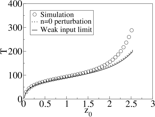
Fig. 6 compares the simulation results and the theoretical predictions based on the perturbation approximation of Eqs. (45) and (52). We see that compared with the weak input limit, the result is improved a little bit.

Refer to caption
Figure 6: The reaction time vs. the jump size. Parameters: the same as Fig. 5.

4.3 The n=5𝑛5n=5 Perturbation

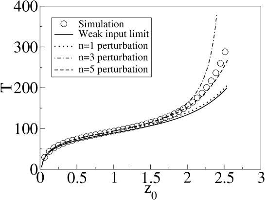
By increasing the order of perturbation, we get an increasingly better approximation of the network dynamics. We observe that the improvement is btter when the order of perturbation n𝑛n increases by 1 to an odd integer. This is because odd distortion modes are antisymmetric, which better approximate the bump’s shape distortion when the position of the external stimulus is biased towards one side of the bump.

Below, we present the results of the n=5𝑛5n=5 perturbation, which correspond to taking into account distortions in the position, height, width, skewness and the fourth- and fifth-order distortions of the bump.

By including perturbations up to n=5𝑛5n=5, Eqs. (37) and (39) become

(ddt+1λ0τ)a0=I0τ+a12adzdt24τa2+632τa4,𝑑𝑑𝑡1subscript𝜆0𝜏subscript𝑎0subscript𝐼0𝜏subscript𝑎12𝑎𝑑𝑧𝑑𝑡24𝜏subscript𝑎2632𝜏subscript𝑎4\displaystyle\left(\frac{d}{dt}+\frac{1-\lambda_{0}}{\tau}\right)a_{0}=\frac{I_{0}}{\tau}+\frac{a_{1}}{2a}\frac{dz}{dt}-\frac{\sqrt{2}}{4\tau}a_{2}+\frac{\sqrt{6}}{32\tau}a_{4}, (53)
da1dt=I1τ((2π)1/2aU0+a02a2)12adzdt68τa3+3064τa5,𝑑subscript𝑎1𝑑𝑡subscript𝐼1𝜏superscript2𝜋12𝑎subscript𝑈0subscript𝑎02subscript𝑎212𝑎𝑑𝑧𝑑𝑡68𝜏subscript𝑎33064𝜏subscript𝑎5\displaystyle\frac{da_{1}}{dt}=\frac{I_{1}}{\tau}-\left(\sqrt{(2\pi)^{1/2}a}U_{0}+a_{0}-\sqrt{2}a_{2}\right)\frac{1}{2a}\frac{dz}{dt}-\frac{\sqrt{6}}{8\tau}a_{3}+\frac{\sqrt{30}}{64\tau}a_{5}, (54)
(ddt+12τ)a2=I2τ2a13a32adzdt38τa4,𝑑𝑑𝑡12𝜏subscript𝑎2subscript𝐼2𝜏2subscript𝑎13subscript𝑎32𝑎𝑑𝑧𝑑𝑡38𝜏subscript𝑎4\displaystyle\left(\frac{d}{dt}+\frac{1}{2\tau}\right)a_{2}=\frac{I_{2}}{\tau}-\frac{\sqrt{2}a_{1}-\sqrt{3}a_{3}}{2a}\frac{dz}{dt}-\frac{\sqrt{3}}{8\tau}a_{4}, (55)
(ddt+34τ)a3=I3τ3a24a42adzdt516τa5,𝑑𝑑𝑡34𝜏subscript𝑎3subscript𝐼3𝜏3subscript𝑎24subscript𝑎42𝑎𝑑𝑧𝑑𝑡516𝜏subscript𝑎5\displaystyle\left(\frac{d}{dt}+\frac{3}{4\tau}\right)a_{3}=\frac{I_{3}}{\tau}-\frac{\sqrt{3}a_{2}-\sqrt{4}a_{4}}{2a}\frac{dz}{dt}-\frac{\sqrt{5}}{16\tau}a_{5}, (56)
(ddt+78τ)a4=I4τ4a35a52adzdt,𝑑𝑑𝑡78𝜏subscript𝑎4subscript𝐼4𝜏4subscript𝑎35subscript𝑎52𝑎𝑑𝑧𝑑𝑡\displaystyle\left(\frac{d}{dt}+\frac{7}{8\tau}\right)a_{4}=\frac{I_{4}}{\tau}-\frac{\sqrt{4}a_{3}-\sqrt{5}a_{5}}{2a}\frac{dz}{dt}, (57)
dzdt=2a(I1+32I3+158I5+a1)τ((2π)1/2aU0+a0+12a2+38a4),𝑑𝑧𝑑𝑡2𝑎subscript𝐼132subscript𝐼3158subscript𝐼5subscript𝑎1𝜏superscript2𝜋12𝑎subscript𝑈0subscript𝑎012subscript𝑎238subscript𝑎4\displaystyle\frac{dz}{dt}=\frac{2a\left(I_{1}+\sqrt{\frac{3}{2}}I_{3}+\sqrt{\frac{15}{8}}I_{5}+a_{1}\right)}{\tau\left(\sqrt{(2\pi)^{1/2}a}U_{0}+a_{0}+\sqrt{\frac{1}{2}}a_{2}+\sqrt{\frac{3}{8}}a_{4}\right)}, (58)

and a5subscript𝑎5a_{5} is determined by the condition a1+3/2a3+15/8a5=0subscript𝑎132subscript𝑎3158subscript𝑎50a_{1}+\sqrt{3/2}a_{3}+\sqrt{15/8}a_{5}=0. Fig. 7 compares the theoretical predictions with the simulation results. They agree very well even when the jump sizes are large.

Refer to caption
Figure 7: The reaction time vs. the jump size. The simulation result is compared with the n=5𝑛5n=5 perturbation approximation. Parameters: the same as Fig. 5. Note that the predictions of the n=0𝑛0n=0 and n=1𝑛1n=1 perturbations are the same because of the self-consistent condition in Eq. (121). Also, the predicted reaction time given by the n=1𝑛1n=1 and n=2𝑛2n=2 perturbations are almost the same. So are the n=3𝑛3n=3 and n=4𝑛4n=4 perturbations.

4.4 Shape Distortion

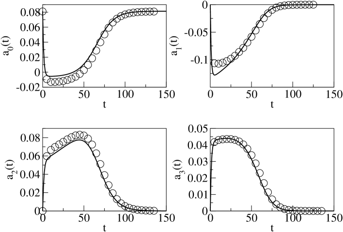
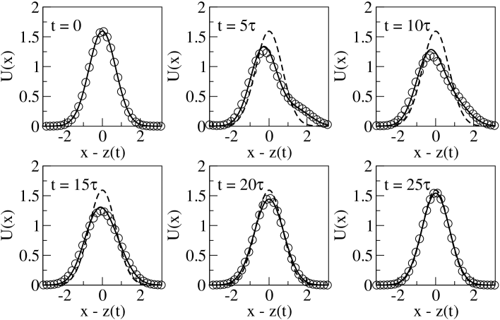
Besides the reaction time, it is instructive to study the distortion in the bump’s shape during tracking. As shown in Fig. 8, there is an abrupt change in the height, position, width and skewness immediately after the external stimulus is abruptly removed at t=0𝑡0t=0. a0(t)subscript𝑎0𝑡a_{0}(t) approaches 0 roughly, as if there were no external stimulus, and there is even a slight overshoot. a1(t)subscript𝑎1𝑡a_{1}(t) also drops abruptly, showing that the peak position lags behind the center of mass, an indication that the bump is abruptly distorted. At the same time, distortions in the width and skewness increase abruptly, showing that the bump is suddenly pulled by the external stimulus from its new position. After the initial abrupt changes, the distorted components undergo rather smooth changes on the journey to the new position. Finally, when the bump approaches its destination, the height returns to its equilibrium value, while the other components approach 0.

We also compare the perturbation and simulation results in Fig. 8. The agreement is very good. Discrepancies arise from linearizing the interaction term in going from Eq. (2) to (6). Their effects are mainly seen in the moments immediately after the abrupt change in the external stimulus.

Figure 9 shows the distorted bump in the center-of-mass frame during tracking. During the process, the lowering of the height, the retarding of the peak position, the broadening of the width, and the skewing due to the attraction of the newly positioned stimulus are clearly visible.
Refer to caption
Figure 8: The first four an(t)subscript𝑎𝑛𝑡a_{n}(t) obtained by the n=10𝑛10n=10 perturbation (dashed lines) and by projecting U(x,t)𝑈𝑥𝑡U(x,t) onto the corresponding vn(x|z)subscript𝑣𝑛conditional𝑥𝑧v_{n}(x|z) during tracking (symbols). Parameters: N=200𝑁200N=200, α=0.05𝛼0.05\alpha=0.05, a=0.5𝑎0.5a=0.5, τ=1𝜏1\tau=1, k=0.5𝑘0.5k=0.5, ρ=N/2π𝜌𝑁2𝜋\rho=N/2\pi and A=2aπ𝐴2𝑎𝜋A=\sqrt{2a}\pi.

Refer to caption
Figure 9: Snapshots of the neuronal inputs in the center-of-mass frame of the bump. Symbols: simulations. Solid lines: predicted synaptic input with the n=10𝑛10n=10 perturbation. Parameters: N=200𝑁200N=200, α=0.15𝛼0.15\alpha=0.15, a=0.5𝑎0.5a=0.5, τ=1𝜏1\tau=1, k=0.5𝑘0.5k=0.5, ρ=N/2π𝜌𝑁2𝜋\rho=N/2\pi and A=2aπ𝐴2𝑎𝜋A=\sqrt{2a}\pi.

5 Dynamics of a Two-Dimensional CANN

We can extend our analysis to a two-dimensional(2D) CANN. Consider a neural ensemble encoding a 2D continuous stimulus 𝐱=(x1,x2)𝐱subscript𝑥1subscript𝑥2{\bf x}=(x_{1},x_{2}), with its components x1(,)subscript𝑥1x_{1}\in(-\infty,\infty) and x2(,)subscript𝑥2x_{2}\in(-\infty,\infty). We denote by U(𝐱)𝑈𝐱U({\bf x}) the synaptic input to neurons having the preferred stimulus 𝐱𝐱{\bf x} and r(𝐱)𝑟𝐱r({\bf x}) the corresponding firing rate. For a solvable model, we consider the network whose dynamics is governed by

τU(𝐱,t)t𝜏𝑈𝐱𝑡𝑡\displaystyle\tau\frac{\partial U({\bf x},t)}{\partial t} =\displaystyle= Iext(𝐱,t)+ρ𝑑𝐱J(𝐱,𝐱)r(𝐱,t)U(𝐱,t),subscript𝐼ext𝐱𝑡𝜌subscriptsuperscriptsubscriptsuperscriptdifferential-dsuperscript𝐱𝐽𝐱superscript𝐱𝑟superscript𝐱𝑡𝑈superscript𝐱𝑡\displaystyle I_{\rm ext}({\bf x},t)+\rho\int^{\infty}_{-\infty}\int^{\infty}_{-\infty}d{\bf x}^{\prime}J({\bf x},{\bf x}^{\prime})r({\bf x}^{\prime},t)-U({\bf x}^{\prime},t), (59)
r(𝐱,t)𝑟𝐱𝑡\displaystyle r({\bf x},t) =\displaystyle= U(𝐱,t)21+kρ𝑑𝐱U(𝐱,t)2,𝑈superscript𝐱𝑡21𝑘𝜌subscriptsuperscriptsubscriptsuperscriptdifferential-dsuperscript𝐱𝑈superscriptsuperscript𝐱𝑡2\displaystyle\frac{U({\bf x},t)^{2}}{1+k\rho\int^{\infty}_{-\infty}\int^{\infty}_{-\infty}d{\bf x}^{\prime}U({\bf x}^{\prime},t)^{2}}, (60)

where τ𝜏\tau is the time constant and ρ𝜌\rho the neural density, and the recurrent interactions are chosen to be

J(𝐱,𝐱)=A2πa2exp[(𝐱𝐱)22a2],𝐽𝐱superscript𝐱𝐴2𝜋superscript𝑎2superscript𝐱superscript𝐱22superscript𝑎2J({\bf x},{\bf x}^{\prime})=\frac{A}{2\pi a^{2}}\exp\left[-\frac{({\bf x}-{\bf x}^{\prime})^{2}}{2a^{2}}\right], (61)

where (𝐱𝐱)2=(x1x1)2+(x2x2)2superscript𝐱superscript𝐱2superscriptsubscript𝑥1superscriptsubscript𝑥12superscriptsubscript𝑥2superscriptsubscript𝑥22({\bf x}-{\bf x}^{\prime})^{2}=(x_{1}-x_{1}^{\prime})^{2}+(x_{2}-x_{2}^{\prime})^{2} is the Euclidean distance between 𝐱𝐱{\bf x} and 𝐱superscript𝐱{\bf x}^{\prime}.

It can be checked that when Iext(𝐱,t)=0subscript𝐼ext𝐱𝑡0I_{\rm ext}({\bf x},t)=0 and 0<k<kcA2ρ/(32πa2)0𝑘subscript𝑘𝑐superscript𝐴2𝜌32𝜋superscript𝑎20<k<k_{c}\equiv A^{2}\rho/(32\pi a^{2}), the network holds a continuous family of stationary states given by

U~(𝐱|𝐳)~𝑈conditional𝐱𝐳\displaystyle\tilde{U}({\bf x}|{\bf z}) =\displaystyle= U0exp[(𝐱𝐳)24a2],subscript𝑈0superscript𝐱𝐳24superscript𝑎2\displaystyle U_{0}\exp\left[-\frac{({\bf x}-{\bf z})^{2}}{4a^{2}}\right], (62)
r~(𝐱|𝐳)~𝑟conditional𝐱𝐳\displaystyle\tilde{r}({\bf x}|{\bf z}) =\displaystyle= r0exp[(𝐱𝐳)22a2],subscript𝑟0superscript𝐱𝐳22superscript𝑎2\displaystyle r_{0}\exp\left[-\frac{({\bf x}-{\bf z})^{2}}{2a^{2}}\right], (63)

where U0=[1+(1k/kc)1/2]A/(8πa2k)subscript𝑈0delimited-[]1superscript1𝑘subscript𝑘𝑐12𝐴8𝜋superscript𝑎2𝑘U_{0}=[1+(1-k/k_{c})^{1/2}]A/(8\pi a^{2}k) and r0=[1+(1k/kc)1/2]/(4πa2kρ)subscript𝑟0delimited-[]1superscript1𝑘subscript𝑘𝑐124𝜋superscript𝑎2𝑘𝜌r_{0}=[1+(1-k/k_{c})^{1/2}]/(4\pi a^{2}k\rho). The parameter 𝐳=(z1,z2)𝐳subscript𝑧1subscript𝑧2{\bf z}=(z_{1},z_{2}) is a free variable, indicating the location of the bump. We note the differences in J(𝐱,𝐱)𝐽𝐱superscript𝐱J({\bf x},{\bf x}^{\prime}), kcsubscript𝑘𝑐k_{c}, U0subscript𝑈0U_{0} and r0subscript𝑟0r_{0} when compared with their values in the 1D case.

We analyze the stability of the bump states, and consider the network state U(𝐱,t)=U~(𝐱|𝐳)+δU(𝐱,t)𝑈𝐱𝑡~𝑈conditional𝐱𝐳𝛿𝑈𝐱𝑡U({\bf x},t)=\tilde{U}({\bf x}|{\bf z})+\delta U({\bf x},t). After linearizing Eq. (59) at U~(𝐱|𝐳)~𝑈conditional𝐱𝐳\tilde{U}({\bf x}|{\bf z}), we get

τtδU(𝐱,t)=𝑑𝐱F(𝐱,𝐱|𝐳)δU(𝐱,t)δU(𝐱,t),𝜏𝑡𝛿𝑈𝐱𝑡subscriptsuperscriptsubscriptsuperscriptdifferential-dsuperscript𝐱𝐹𝐱conditionalsuperscript𝐱𝐳𝛿𝑈superscript𝐱𝑡𝛿𝑈𝐱𝑡\tau\frac{\partial}{\partial t}\delta U({\bf x},t)=\int^{\infty}_{-\infty}\int^{\infty}_{-\infty}d{\bf x}^{\prime}F({\bf x},{\bf x}^{\prime}|{\bf z})\delta U({\bf x}^{\prime},t)-\delta U({\bf x},t), (64)

where the interaction kernel is given by

F(𝐱,𝐱|𝐳)𝐹𝐱conditionalsuperscript𝐱𝐳\displaystyle F({\bf x},{\bf x}^{\prime}|{\bf z}) =\displaystyle= 2a2πexp[(𝐱𝐱)22a2]exp[(𝐱𝐳)24a2],2superscript𝑎2𝜋superscript𝐱superscript𝐱22superscript𝑎2superscriptsuperscript𝐱𝐳24superscript𝑎2\displaystyle\frac{2}{a^{2}\pi}\exp\left[-\frac{({\bf x}-{\bf x}^{\prime})^{2}}{2a^{2}}\right]\exp\left[-\frac{({\bf x}^{\prime}-{\bf z})^{2}}{4a^{2}}\right], (65)
\displaystyle- 1+1k/kc2πa2exp[(𝐱𝐳)24a2]exp[(𝐱𝐳)24a2].11𝑘subscript𝑘𝑐2𝜋superscript𝑎2superscript𝐱𝐳24superscript𝑎2superscriptsuperscript𝐱𝐳24superscript𝑎2\displaystyle{\frac{1+\sqrt{1-k/k_{c}}}{2\pi a^{2}}}\exp\left[-\frac{({\bf x}-{\bf z})^{2}}{4a^{2}}\right]\exp\left[-\frac{({\bf x}^{\prime}-{\bf z})^{2}}{4a^{2}}\right].

We can construct the right eigenfunction of F(𝐱,𝐱|𝐳)𝐹𝐱conditionalsuperscript𝐱𝐳F({\bf x},{\bf x}^{\prime}|{\bf z}) by using the product of the eigenfunctions un(x|z)subscript𝑢𝑛conditional𝑥𝑧u_{n}(x|z) in the 1D case, i.e.,

um,n(𝐱|𝐳)=um(x1|z1)un(x2|z2),m,n=0,1,2,.formulae-sequencesubscript𝑢𝑚𝑛conditional𝐱𝐳subscript𝑢𝑚conditionalsubscript𝑥1subscript𝑧1subscript𝑢𝑛conditionalsubscript𝑥2subscript𝑧2𝑚𝑛012u_{m,n}({\bf x}|{\bf z})=u_{m}(x_{1}|z_{1})u_{n}(x_{2}|z_{2}),~{}~{}m,n=0,1,2,\ldots. (66)

The corresponding eigenvalues are given by (see Appendix F)

λ0,0subscript𝜆00\displaystyle\lambda_{0,0} =\displaystyle= λ0subscript𝜆0\displaystyle\lambda_{0} (67)
λm,0subscript𝜆𝑚0\displaystyle\lambda_{m,0} =\displaystyle= λm,m0,subscript𝜆𝑚𝑚0\displaystyle\lambda_{m},~{}~{}m\neq 0, (68)
λ0,nsubscript𝜆0𝑛\displaystyle\lambda_{0,n} =\displaystyle= λn,n0,subscript𝜆𝑛𝑛0\displaystyle\lambda_{n},~{}~{}n\neq 0, (69)
λm,nsubscript𝜆𝑚𝑛\displaystyle\lambda_{m,n} =\displaystyle= λmλn,m0,n0,formulae-sequencesubscript𝜆𝑚subscript𝜆𝑛𝑚0𝑛0\displaystyle\lambda_{m}\lambda_{n},~{}~{}m\neq 0,n\neq 0, (70)

where λmsubscript𝜆𝑚\lambda_{m} are the eigenvalues in the 1D case given by Eqs. (15) and (16).

The eigenfunction u0,0(𝐱|𝐳)subscript𝑢00conditional𝐱𝐳u_{0,0}({\bf x}|{\bf z}) corresponds to the amplitude mode of the 2D bump state of the network. u1,0(𝐱|𝐳)subscript𝑢10conditional𝐱𝐳u_{1,0}({\bf x}|{\bf z}) corresponds to the displacement of the bump position along the coordinate z1subscript𝑧1z_{1} and u0,1(𝐱|𝐳)subscript𝑢01conditional𝐱𝐳u_{0,1}({\bf x}|{\bf z}) the positional shift along z2subscript𝑧2z_{2}. A linear combination of u1,0(𝐱|𝐳)subscript𝑢10conditional𝐱𝐳u_{1,0}({\bf x}|{\bf z}) and u0,1(𝐱|𝐳)subscript𝑢01conditional𝐱𝐳u_{0,1}({\bf x}|{\bf z}), i.e., c1u1,0(𝐱|𝐳)+c2u0,1(𝐱,𝐳)subscript𝑐1subscript𝑢10conditional𝐱𝐳subscript𝑐2subscript𝑢01𝐱𝐳c_{1}u_{1,0}({\bf x}|{\bf z})+c_{2}u_{0,1}({\bf x},{\bf z}), with c1subscript𝑐1c_{1} and c2subscript𝑐2c_{2} being constants and satisfying c12+c22=1superscriptsubscript𝑐12superscriptsubscript𝑐221c_{1}^{2}+c_{2}^{2}=1, corresponds to the positional shift of the bump along the 𝐜=(c1,c2)𝐜subscript𝑐1subscript𝑐2{\bf c}=(c_{1},c_{2}) direction. Interestingly, the eigenvalue for c1u1,0(𝐱|𝐳)+c2u0,1(𝐱,𝐳)subscript𝑐1subscript𝑢10conditional𝐱𝐳subscript𝑐2subscript𝑢01𝐱𝐳c_{1}u_{1,0}({\bf x}|{\bf z})+c_{2}u_{0,1}({\bf x},{\bf z}) is 1, indicating that the bump is neutrally stable in the two-dimensional space 𝐳𝐳{\bf z}.

Analogous to the 1D case, we can develop a perturbation method to solve the network dynamics, e.g., by using the 2D wave functions, vm,n(𝐱|𝐳)=vn(x1|z1)vn(x2|z2)subscript𝑣𝑚𝑛conditional𝐱𝐳subscript𝑣𝑛conditionalsubscript𝑥1subscript𝑧1subscript𝑣𝑛conditionalsubscript𝑥2subscript𝑧2v_{m,n}({\bf x}|{\bf z})=v_{n}(x_{1}|z_{1})v_{n}(x_{2}|z_{2}), of the quantum harmonic oscillators as the basis functions. A more comprehensive treatment of the problem involves transforming the basis functions to polar coordinates; it will be presented elsewhere. Here, as an illustration, we will present only the result for the weak input limit in the rectilinear coordinates, which corrsponds to projecting the network dynamics on a single displacement mode. We choose the external input to be

Iext(𝐱,t)=αU0exp[(𝐱𝐳0)24a2]+ση(𝐱,t),subscript𝐼ext𝐱𝑡𝛼subscript𝑈0superscript𝐱superscript𝐳024superscript𝑎2𝜎𝜂𝐱𝑡I_{\rm ext}({\bf x},t)=\alpha U_{0}\exp\left[-{\frac{({\bf x}-{\bf z}^{0})^{2}}{4a^{2}}}\right]+\sigma\eta({\bf x},t), (71)

where 𝐳0superscript𝐳0{\bf z}^{0} represents the stimulus location.

Suppose the bump position is 𝐳(t)𝐳𝑡{\bf z}(t) at time t𝑡t. Then, the stimulus will pull the bump towards the location 𝐳0superscript𝐳0{\bf z}^{0}. In the limit of weak inputs, the network dynamics is dominated by the positional shift of the bump along the straight line through 𝐳0superscript𝐳0{\bf z}^{0}. As derived in Appendix F,

d(𝐳𝐳0)dt=ατ(𝐳𝐳0)exp[(𝐳𝐳0)28a2]+2Dη(t),𝑑𝐳superscript𝐳0𝑑𝑡𝛼𝜏𝐳superscript𝐳0superscript𝐳superscript𝐳028superscript𝑎22𝐷𝜂𝑡\frac{d({\bf z}-{\bf z}^{0})}{dt}=\frac{\alpha}{\tau}({\bf z}-{\bf z}^{0})\exp\left[-\frac{({\bf z}-{\bf z}^{0})^{2}}{8a^{2}}\right]+\sqrt{2D}\eta(t), (72)

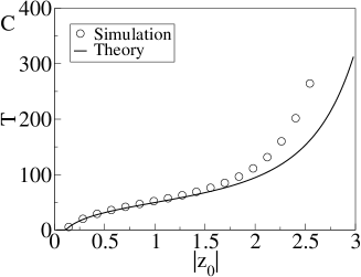
where D=σ2/(U02τ2π)𝐷superscript𝜎2superscriptsubscript𝑈02superscript𝜏2𝜋D=\sigma^{2}/(U_{0}^{2}\tau^{2}\pi). This equation describes how the distance between the bump and the stimulus varies with time. It has the same form as Eq. (26) except that zz0𝑧superscript𝑧0z-z^{0} is replaced by 𝐳𝐳0𝐳superscript𝐳0{\bf z}-{\bf z}^{0}. Thus, the network exhibits the same dynamical properties as observed in the 1D case. Fig. 10 compares the theoretical predictions and the simulation results of the reaction time of the 2D CANN. As expected, they agree with each other very well with small jump sizes.


Refer to caption
Refer to caption
Refer to caption
Figure 10: (A) The stationary state of the 2D CANN. (B) Illustrating the tracking process of the network; (C) The reaction time vs. the jump size. The simulation result is compared with the theoretical prediction. Parameters: N=40×40𝑁4040N=40\times 40, k=0.5𝑘0.5k=0.5, a=0.5𝑎0.5a=0.5, τ=1𝜏1\tau=1, A=2πa2𝐴2𝜋superscript𝑎2A=\sqrt{2}\pi a^{2}, ρ=N/(2π)2𝜌𝑁superscript2𝜋2\rho=N/(2\pi)^{2}, α=0.05𝛼0.05\alpha=0.05 and θ=2π/N𝜃2𝜋𝑁\theta=\sqrt{2}\pi/N.

6 Discussion and Conclusions

The idea that the landscape of the energy function of a CANN has a canyon structure, which facilitates the tracking capacity of a neural system has long been recognized (see, e.g., [Amari 1977, Hansel and Sompolinsky 1998, Brody, Romo, and Kepecs 2003, Wu and Amari 2005]). However, a detailed and rigorous analysis of this property has been lacking. The main challenge here is to solve the network dynamics analytically, elucidating how the shape of the network state is affected during the tracking. In this study, by using a simple analytically solvable model, we systematically investigate this issue. There are two parts to our main results. First, we show that the dynamics of a CANN can be decomposed into different motion modes, corresponding to distortions in the height, position, width, skewness and other higher-order distortions in the shape of the bump states. We demonstrate that with a CANN, it is the positional shift that dominates the network dynamics, with other motion modes having high-order contributions. Second, we develop a time-dependent perturbation approach to approximate the network dynamics. Geometrically, this corresponds to projecting the network dynamics onto its dominating motion modes. Simulation results confirm that our method works very well. Two interesting phenomena in the tracking performance of a CANN are observed, namely, the maximum trackable speed and the logarithmic reaction time of the network. Since both properties are associated with the unique dynamics of a CANN, they may be tested in practice and serve as clues for checking the application of a CANN in neural systems.

To facilitate an analytical solution and hence to describe the network dynamics clearly, we have used a simple firing-rate-based model with the inhibition effect in the form of divisive normalization, and the generality of our results may thus be a concern. In particular, we should consider whether the mechanism of divisive normalization is plausible, whether tracking behavior can be observed in models with different inhibitory mechanisms, and how the perturbation method developed in this paper can be used in other types of networks.

First, we argue that a neural system can have resources to implement divisive normalization [Grossberg 1988, Heeger 1993, Deneve, Latham, and Pouget 1999]. Let us consider a network in which all excitatory neurons are connected to a pool of inhibitory neurons. If the time constant of inhibitory neurons is much smaller than that of excitatory neurons, and if these inhibitory neurons inhibit the activity of the excitatory neurons in a uniform shunting way, then the effect of divisive normalization can be achieved.

Second, even if there exists uncertainty of the model, the main conclusions of tracking behavior in this work are applicable to general cases. This is because our calculation is based on the fact that the dynamics of a CANN is largely dominated by the positional shift of the network states, a property coming from the translational invariance of the neuronal interactions, rather than from the inhibition mechanism. To see this point clearly, let us consider the dynamics of a network having the same form as Eq. (2), but the exact form of the inihibition mechansim remains unspecified. We consider J(xx)𝐽𝑥superscript𝑥J(x-x^{\prime}) and r(x)𝑟𝑥r(x) that are properly chosen (e.g., J(xx)𝐽𝑥superscript𝑥J(x-x^{\prime}) is of the Mexcian-hat shape and r(x)𝑟𝑥r(x) a sigmoid function of the inputs), so that the network holds a continuous family of stationary states, denoted as U~(x|z)~𝑈conditional𝑥𝑧\tilde{U}(x|z) and r~(x|z)~𝑟conditional𝑥𝑧\tilde{r}(x|z), with z𝑧z representing the bump position. This implies that

U~(x|z)=ρ𝑑xJ(xx)r~(x|z).~𝑈conditional𝑥𝑧𝜌subscriptsuperscriptdifferential-dsuperscript𝑥𝐽𝑥superscript𝑥~𝑟conditionalsuperscript𝑥𝑧\tilde{U}(x|z)=\rho\int^{\infty}_{-\infty}dx^{\prime}J(x-x^{\prime})\tilde{r}(x^{\prime}|z). (73)

By differentiating both sides of the above equation with respect to z𝑧z, we get

U~(x|z)z~𝑈conditional𝑥𝑧𝑧\displaystyle\frac{\partial\tilde{U}(x|z)}{\partial z} =\displaystyle= ρ𝑑x𝑑x′′J(xx)r~(x|z)U~(x′′|z)U~(x′′|z)z𝜌subscriptsuperscriptdifferential-dsuperscript𝑥subscriptsuperscriptdifferential-dsuperscript𝑥′′𝐽𝑥superscript𝑥~𝑟conditionalsuperscript𝑥𝑧~𝑈conditionalsuperscript𝑥′′𝑧~𝑈conditionalsuperscript𝑥′′𝑧𝑧\displaystyle\rho\int^{\infty}_{-\infty}dx^{\prime}\int^{\infty}_{-\infty}dx^{\prime\prime}J(x-x^{\prime})\frac{\partial\tilde{r}(x^{\prime}|z)}{\partial\tilde{U}(x^{\prime\prime}|z)}\frac{\partial\tilde{U}(x^{\prime\prime}|z)}{\partial z} (74)
=\displaystyle= 𝑑x′′F(x,x′′|z)U~(x′′|z)z.subscriptsuperscriptdifferential-dsuperscript𝑥′′𝐹𝑥conditionalsuperscript𝑥′′𝑧~𝑈conditionalsuperscript𝑥′′𝑧𝑧\displaystyle\int^{\infty}_{-\infty}dx^{\prime\prime}F(x,x^{\prime\prime}|z)\frac{\partial\tilde{U}(x^{\prime\prime}|z)}{\partial z}.

Thus, the mode of the positional shift of the bump, U~(x|z)/z~𝑈conditional𝑥𝑧𝑧\partial\tilde{U}(x|z)/\partial z, is the eigenfunction of the interaction kernel F𝐹F with the eigenvalue equal to 1. We should observe similar tracking behavior of the network, once J(xx)𝐽𝑥superscript𝑥J(x-x^{\prime}) and r(x)𝑟𝑥r(x) are properly chosen to ensure that all the other eigenvalues are less than one.

Third, the perturbation method developed in this paper can be used to analyze other types of networks with tracking behavior. Consider appropriate choices of J(xx)𝐽𝑥superscript𝑥J(x-x^{\prime}) and r(x)𝑟𝑥r(x) that can hold a continuous family of bump states centered at position z𝑧z (for example, J(xx)𝐽𝑥superscript𝑥J(x-x^{\prime}) having a Mexican-hat shape and r(U)𝑟𝑈r(U) a sigmoid function). Then, the dynamics of the bump can be described by Eq. (6), with

F(x,x|z)=𝑑xJ(xx)r(U~(x|z))U~(x|z).𝐹𝑥conditionalsuperscript𝑥𝑧subscriptsuperscriptdifferential-dsuperscript𝑥𝐽𝑥superscript𝑥𝑟~𝑈conditionalsuperscript𝑥𝑧~𝑈conditionalsuperscript𝑥𝑧F(x,x^{\prime}|z)=\int^{\infty}_{-\infty}dx^{\prime}J(x-x^{\prime})\frac{\partial r(\tilde{U}(x^{\prime}|z))}{\partial\tilde{U}(x^{\prime}|z)}. (75)

Using the basis functions of the quantum harmonic oscillator, we can obtain the matrix elements Fmnsubscript𝐹𝑚𝑛F_{mn} from Eq. (13). While elegant expressions such as those in Eq. (14) may not be available in the general case, we can nevertheless compute Fmnsubscript𝐹𝑚𝑛F_{mn} numerically. Perturbation dynamics similar to Eqs. (37) and (39) can be worked out following Appendix D. Indeed, we have considered networks with Mexican-hat-shaped interactions. Tracking dynamics with a logarithmic reaction time and a maximum trackable speed is observed, and the convergence of the perturbation method is equally remarkable. These results will be reported elsewhere.

The tracking dynamics of a CANN has also been studied by other authors. In particular, Zhang proposed a mechanism of using asymmetrical recurrent interactions to drive the bump, so that the shape distortion would be minimized [Zhang 1996]. Xie et al further proposed a double ring network model that uses the inputs from the vestibular system in mammals to achieve these asymmetrical interactions [Xie, Hahnloser, and Seung 2002]. This mechansim works well for the head-direction system, but it is unclear if it can be achieved in other neural systems. For instance, in the visual and hippocampal systems, it is often assumed that the bump movement is directly driven by external inputs (see, e.g., [Samsonovich and McNaughton 1997, Berry II, Brivanlou, Jordon, and Meister 1999, Fu, Shen, and Dan 2001]), and the distortion of the bump is inevitable (indeed the bump distortions in [Berry II, Brivanlou, Jordon, and Meister 1999, Fu, Shen, and Dan 2001] are associated with visual perception). The contribution of this study is that we quantify how the distortion of the bump’s shape affects the network tracking performance, and we obtain the maximum trackable speed of the network. We hope that this study will enrich our knowledge about the tracking dynamics of a CANN, which may differ in different brain functions. Apart from the tracking capacity, recent experimental observations have suggested that CANNs may have other important roles in neural cognitive functions. For example, the highly structured state space of a CANN may provide a neural basis of encoding the categorization relationships of objects [Jastorff, Kourtzi, and Giese 2006, Graf, Wichmann, Bulthoff, and Scholkopf 2006]. It is quite possible that the distance between two memory states in the canyon defines the perceptual similarity between the two objects. We will explore these issues in the future, and we expect that the theoretical model and approaches developed in this work will provide valuable tools.

Acknowledgment

This work was partially supported by the Research Grants Council of Hong Kong (Grant Nos. HKUST 603606, 603607 and 604008), and BBSRC (BB/E017436/1) and the Royal Society of UK.

Appendix A: The Hermite Polynomials

Since the Hermite polynomials are frequently used in the calculations of this paper, here we summarize their main properties for the convenience of the reader.

The n𝑛nth-order Hermite polynomial is defined as

Hn(x)=(1)nexp(x2)(ddx)nexp(x2).subscript𝐻𝑛𝑥superscript1𝑛superscript𝑥2superscript𝑑𝑑𝑥𝑛superscript𝑥2H_{n}(x)=(-1)^{n}\exp(x^{2})\left(\frac{d}{dx}\right)^{n}\exp(-x^{2}). (76)

The first five Hermite polynomials are given by H0(x)=1subscript𝐻0𝑥1H_{0}(x)=1, H1(x)=2xsubscript𝐻1𝑥2𝑥H_{1}(x)=2x, H2(x)=4x22subscript𝐻2𝑥4superscript𝑥22H_{2}(x)=4x^{2}-2, H3(x)=8x312xsubscript𝐻3𝑥8superscript𝑥312𝑥H_{3}(x)=8x^{3}-12x, H4(x)=16x448x2+12subscript𝐻4𝑥16superscript𝑥448superscript𝑥212H_{4}(x)=16x^{4}-48x^{2}+12. For the analysis in this paper, it is instructive to note that the Hermite polynomials satisfy the following properties.

  • Recursion relation:

    Hn+1(x)subscript𝐻𝑛1𝑥\displaystyle H_{n+1}(x) =\displaystyle= 2xHn(x)Hn(x),2𝑥subscript𝐻𝑛𝑥subscriptsuperscript𝐻𝑛𝑥\displaystyle 2xH_{n}(x)-H^{\prime}_{n}(x), (77)
    Hn(x)subscriptsuperscript𝐻𝑛𝑥\displaystyle H^{\prime}_{n}(x) =\displaystyle= 2nHn1(x),2𝑛subscript𝐻𝑛1𝑥\displaystyle 2nH_{n-1}(x), (78)
    Hn(x+y)subscript𝐻𝑛𝑥𝑦\displaystyle H_{n}(x+y) =\displaystyle= k=0n(nk)Hk(x)(2y)nk.superscriptsubscript𝑘0𝑛𝑛𝑘subscript𝐻𝑘𝑥superscript2𝑦𝑛𝑘\displaystyle\sum_{k=0}^{n}\left(\begin{array}[]{c}n\\ k\end{array}\right)H_{k}(x)(2y)^{n-k}. (81)
  • Contour integral representation:

    Hn(x)=n!dt2πitn+1e2txt2,subscript𝐻𝑛𝑥𝑛contour-integral𝑑𝑡2𝜋𝑖superscript𝑡𝑛1superscript𝑒2𝑡𝑥superscript𝑡2H_{n}(x)=n!\oint\frac{dt}{2\pi it^{n+1}}e^{2tx-t^{2}}, (82)

    with the contour encircling the origin.

Appendix B: The Interaction Kernel F(x,x|z)𝐹𝑥conditionalsuperscript𝑥𝑧F(x,x^{\prime}|z)

Linearizing Eq. (2) at U~(x|z)~𝑈conditional𝑥𝑧\tilde{U}(x|z), we arrive at

τtδU(x)𝜏𝑡𝛿𝑈𝑥\displaystyle\tau\frac{\partial}{\partial t}\delta U(x) =\displaystyle= ρdxJ(x,x)[2U(x)BδU(x)\displaystyle\rho\int^{\infty}_{-\infty}dx^{\prime}J(x,x^{\prime})\left[\frac{2U(x^{\prime})}{B}\delta U(x^{\prime})\right. (83)
\displaystyle- U(x)2B2dx′′2kρU(x′′)δU(x′′)]δU(x),\displaystyle\left.\frac{U(x^{\prime})^{2}}{B^{2}}\int^{\infty}_{-\infty}dx^{\prime\prime}2k\rho U(x^{\prime\prime})\delta U(x^{\prime\prime})\right]-\delta U(x),

where we have dropped the dependence on t𝑡t for brevity, and B=1+kρ𝑑xU~(x)2=ρAU0/2𝐵1𝑘𝜌subscriptsuperscriptdifferential-dsuperscript𝑥~𝑈superscriptsuperscript𝑥2𝜌𝐴subscript𝑈02B=1+k\rho\int^{\infty}_{-\infty}dx^{\prime}\tilde{U}(x^{\prime})^{2}=\rho AU_{0}/\sqrt{2}. Interchanging the dummy variables xsuperscript𝑥x^{\prime} and x′′superscript𝑥′′x^{\prime\prime} in the last term, we obtain Eqs. (6) and (7), with

F(x,x|z)𝐹𝑥conditionalsuperscript𝑥𝑧\displaystyle F(x,x^{\prime}|z) =\displaystyle= 2aπexp[(xx)22a2]exp[(xz)24a2]2𝑎𝜋superscript𝑥superscript𝑥22superscript𝑎2superscriptsuperscript𝑥𝑧24superscript𝑎2\displaystyle{\frac{2}{a\sqrt{\pi}}}\exp\left[-\frac{(x-x^{\prime})^{2}}{2a^{2}}\right]\exp\left[-\frac{(x^{\prime}-z)^{2}}{4a^{2}}\right] (84)
\displaystyle- 1+1k/kc2πaexp[(xz)24a2]exp[(xz)24a2].11𝑘subscript𝑘𝑐2𝜋𝑎superscript𝑥𝑧24superscript𝑎2superscriptsuperscript𝑥𝑧24superscript𝑎2\displaystyle{\frac{1+\sqrt{1-k/k_{c}}}{\sqrt{2\pi}a}}\exp\left[-\frac{(x-z)^{2}}{4a^{2}}\right]\exp\left[-\frac{(x^{\prime}-z)^{2}}{4a^{2}}\right].

By substituting the expressions of U(x)𝑈𝑥U(x), J(x,x)𝐽𝑥superscript𝑥J(x,x^{\prime}) and r(x)𝑟𝑥r(x), we get Eq. (7).

To calculate the matrix elements Fmnsubscript𝐹𝑚𝑛F_{mn} in Eq. (13), we denote

gn(x|z)=𝑑xF(x,x|z)vn(x|z).subscript𝑔𝑛conditional𝑥𝑧subscriptsuperscriptdifferential-dsuperscript𝑥𝐹𝑥conditionalsuperscript𝑥𝑧subscript𝑣𝑛conditionalsuperscript𝑥𝑧g_{n}(x|z)=\int^{\infty}_{-\infty}dx^{\prime}F(x,x^{\prime}|z)v_{n}(x^{\prime}|z). (85)

From Eqs. (7) and (8),

gn(x|z)subscript𝑔𝑛conditional𝑥𝑧\displaystyle g_{n}(x|z) =\displaystyle= (1)n2(2a)n12aπ3/2n!2n𝑑xexp[(xx)22a2](ddx)nexp[(xz)22a2]superscript1𝑛2superscript2𝑎𝑛12𝑎superscript𝜋32𝑛superscript2𝑛subscriptsuperscriptdifferential-dsuperscript𝑥superscript𝑥superscript𝑥22superscript𝑎2superscript𝑑𝑑superscript𝑥𝑛superscriptsuperscript𝑥𝑧22superscript𝑎2\displaystyle\frac{(-1)^{n}2(\sqrt{2}a)^{n-\frac{1}{2}}}{a\sqrt{\pi^{3/2}n!2^{n}}}\int^{\infty}_{-\infty}dx^{\prime}\exp\left[-\frac{(x-x^{\prime})^{2}}{2a^{2}}\right]\left(\frac{d}{dx^{\prime}}\right)^{n}\exp\left[-\frac{(x^{\prime}-z)^{2}}{2a^{2}}\right] (86)
(1+1k/kc)(1)n(2a)n12aπ3/2n!2n+1exp[(xz)24a2]11𝑘subscript𝑘𝑐superscript1𝑛superscript2𝑎𝑛12𝑎superscript𝜋32𝑛superscript2𝑛1superscript𝑥𝑧24superscript𝑎2\displaystyle-\frac{(1+\sqrt{1-k/k_{c}})(-1)^{n}(\sqrt{2}a)^{n-\frac{1}{2}}}{a\sqrt{\pi^{3/2}n!2^{n+1}}}\exp\left[-\frac{(x-z)^{2}}{4a^{2}}\right]
×dx(ddx)nexp[(xz)22a2].\displaystyle\times\int^{\infty}_{-\infty}dx^{\prime}\left(\frac{d}{dx^{\prime}}\right)^{n}\exp\left[-\frac{(x^{\prime}-z)^{2}}{2a^{2}}\right].

The second term vanishes for n1𝑛1n\geq 1. Hence, by evaluating the two integrals explicitly for n=0𝑛0n=0, we have

g0(x|z)=(11k/kc)v0(x|z).subscript𝑔0conditional𝑥𝑧11𝑘subscript𝑘𝑐subscript𝑣0conditional𝑥𝑧g_{0}(x|z)=(1-\sqrt{1-k/k_{c}})v_{0}(x|z). (87)

Making use of the orthonormality of the basis vn(x|z)subscript𝑣𝑛conditional𝑥𝑧v_{n}(x|z), we obtain the first line of Eq. (14).

Next, we consider the case n1𝑛1n\geq 1, focusing on the first term.

Utilizing the identity (d/dz)ne(xz)2/2a2=(d/dx)ne(xz)2/2a2superscript𝑑𝑑𝑧𝑛superscript𝑒superscript𝑥𝑧22superscript𝑎2superscript𝑑𝑑𝑥𝑛superscript𝑒superscript𝑥𝑧22superscript𝑎2(-d/dz)^{n}e^{-(x-z)^{2}/2a^{2}}=(d/dx)^{n}e^{-(x-z)^{2}/2a^{2}}, we have

gn(x|z)=(1)n2(2a)n12aπ3/2n!2n(ddz)n𝑑xexp[(xx)22a2]exp[(xz)22a2].subscript𝑔𝑛conditional𝑥𝑧superscript1𝑛2superscript2𝑎𝑛12𝑎superscript𝜋32𝑛superscript2𝑛superscript𝑑𝑑𝑧𝑛subscriptsuperscriptdifferential-dsuperscript𝑥superscript𝑥superscript𝑥22superscript𝑎2superscriptsuperscript𝑥𝑧22superscript𝑎2g_{n}(x|z)=\frac{(-1)^{n}2(\sqrt{2}a)^{n-\frac{1}{2}}}{a\sqrt{\pi^{3/2}n!2^{n}}}\left(-\frac{d}{dz}\right)^{n}\int^{\infty}_{-\infty}dx^{\prime}\exp\left[-\frac{(x-x^{\prime})^{2}}{2a^{2}}\right]\exp\left[-\frac{(x^{\prime}-z)^{2}}{2a^{2}}\right]. (88)

Evaluating the integral explicitly, we find that

gn(x|z)=(1)n2(2a)n12π1/2n!2n(ddx)nexp[(xz)24a2].subscript𝑔𝑛conditional𝑥𝑧superscript1𝑛2superscript2𝑎𝑛12superscript𝜋12𝑛superscript2𝑛superscript𝑑𝑑𝑥𝑛superscript𝑥𝑧24superscript𝑎2g_{n}(x|z)=\frac{(-1)^{n}2(\sqrt{2}a)^{n-\frac{1}{2}}}{\sqrt{\pi^{1/2}n!2^{n}}}\left(\frac{d}{dx}\right)^{n}\exp\left[-\frac{(x-z)^{2}}{4a^{2}}\right]. (89)

We are now ready to derive Fmnsubscript𝐹𝑚𝑛F_{mn} from gn(x|z)subscript𝑔𝑛conditional𝑥𝑧g_{n}(x|z):

Fmn=𝑑xvm(x|z)gn(x|z).subscript𝐹𝑚𝑛subscriptsuperscriptdifferential-d𝑥subscript𝑣𝑚conditional𝑥𝑧subscript𝑔𝑛conditional𝑥𝑧F_{mn}=\int^{\infty}_{-\infty}dxv_{m}(x|z)g_{n}(x|z). (90)

From Eqs. (8) and (88),

Fmnsubscript𝐹𝑚𝑛\displaystyle F_{mn} =\displaystyle= 2(1)m(2a)m12π1/2m!2m(1)n(2a)n12π1/2n!2n2superscript1𝑚superscript2𝑎𝑚12superscript𝜋12𝑚superscript2𝑚superscript1𝑛superscript2𝑎𝑛12superscript𝜋12𝑛superscript2𝑛\displaystyle 2\frac{(-1)^{m}(\sqrt{2}a)^{m-\frac{1}{2}}}{\sqrt{\pi^{1/2}m!2^{m}}}\frac{(-1)^{n}(\sqrt{2}a)^{n-\frac{1}{2}}}{\sqrt{\pi^{1/2}n!2^{n}}} (91)
×dxexp[(xz)24a2](ddx)mexp[(xz)22a2](ddx)nexp[(xz)24a2].\displaystyle\times\int^{\infty}_{-\infty}dx\exp\left[\frac{(x-z)^{2}}{4a^{2}}\right]\left(\frac{d}{dx}\right)^{m}\exp\left[-\frac{(x-z)^{2}}{2a^{2}}\right]\left(\frac{d}{dx}\right)^{n}\exp\left[-\frac{(x-z)^{2}}{4a^{2}}\right].

Using the definition of the Hermite polynomials in Eq. (76), this simplfies to

Fmn=2(1)m(2a)m+n1πm!n!2m+n1(2a)n𝑑xHn(xz2a)(ddx)mexp[(xz)22a2].subscript𝐹𝑚𝑛2superscript1𝑚superscript2𝑎𝑚𝑛1𝜋𝑚𝑛superscript2𝑚𝑛1superscript2𝑎𝑛subscriptsuperscriptdifferential-d𝑥subscript𝐻𝑛𝑥𝑧2𝑎superscript𝑑𝑑𝑥𝑚superscript𝑥𝑧22superscript𝑎2F_{mn}=2\frac{(-1)^{m}(\sqrt{2}a)^{m+n-1}}{\sqrt{\pi m!n!2^{m+n}}}\frac{1}{(2a)^{n}}\int^{\infty}_{-\infty}dxH_{n}\left(\frac{x-z}{2a}\right)\left(\frac{d}{dx}\right)^{m}\exp\left[-\frac{(x-z)^{2}}{2a^{2}}\right]. (92)

Applying integration by parts m𝑚m times yields

Fmn=2(2a)m+n1πm!n!2m+n1(2a)n𝑑xexp[(xz)22a2](ddx)mHn(xz2a).subscript𝐹𝑚𝑛2superscript2𝑎𝑚𝑛1𝜋𝑚𝑛superscript2𝑚𝑛1superscript2𝑎𝑛subscriptsuperscriptdifferential-d𝑥superscript𝑥𝑧22superscript𝑎2superscript𝑑𝑑𝑥𝑚subscript𝐻𝑛𝑥𝑧2𝑎F_{mn}=2\frac{(\sqrt{2}a)^{m+n-1}}{\sqrt{\pi m!n!2^{m+n}}}\frac{1}{(2a)^{n}}\int^{\infty}_{-\infty}dx\exp\left[-\frac{(x-z)^{2}}{2a^{2}}\right]\left(\frac{d}{dx}\right)^{m}H_{n}\left(\frac{x-z}{2a}\right). (93)

Applying Eq. (78) m𝑚m times yields, for nm𝑛𝑚n\geq m,

Fmn=2(2a)m+n1πm!n!2m+n1(2a)nn!am(nm)!𝑑xexp[(xz)22a2]Hnm(xz2a),subscript𝐹𝑚𝑛2superscript2𝑎𝑚𝑛1𝜋𝑚𝑛superscript2𝑚𝑛1superscript2𝑎𝑛𝑛superscript𝑎𝑚𝑛𝑚subscriptsuperscriptdifferential-d𝑥superscript𝑥𝑧22superscript𝑎2subscript𝐻𝑛𝑚𝑥𝑧2𝑎F_{mn}=2\frac{(\sqrt{2}a)^{m+n-1}}{\sqrt{\pi m!n!2^{m+n}}}\frac{1}{(2a)^{n}}\frac{n!}{a^{m}(n-m)!}\int^{\infty}_{-\infty}dx\exp\left[-\frac{(x-z)^{2}}{2a^{2}}\right]H_{n-m}\left(\frac{x-z}{2a}\right), (94)

and Fmn=0subscript𝐹𝑚𝑛0F_{mn}=0 otherwise.

Introducing the contour integral representation in Eq. (82) leads to

Fmn=2n!2naπm!𝑑xexp[(xz)22a2]dt2πitnm+1exp[t2+t(xza)].subscript𝐹𝑚𝑛2𝑛superscript2𝑛𝑎𝜋𝑚subscriptsuperscriptdifferential-d𝑥superscript𝑥𝑧22superscript𝑎2contour-integral𝑑𝑡2𝜋𝑖superscript𝑡𝑛𝑚1superscript𝑡2𝑡𝑥𝑧𝑎F_{mn}=\frac{\sqrt{2}\sqrt{n!}}{2^{n}a\sqrt{\pi m!}}\int^{\infty}_{-\infty}dx\exp\left[-\frac{(x-z)^{2}}{2a^{2}}\right]\oint\frac{dt}{2\pi it^{n-m+1}}\exp\left[-t^{2}+t\left(\frac{x-z}{a}\right)\right]. (95)

Interchanging the order of integrating x𝑥x and t𝑡t, we have

Fmn=21nn!m!dt2πitnm+1exp(t22).subscript𝐹𝑚𝑛superscript21𝑛𝑛𝑚contour-integral𝑑𝑡2𝜋𝑖superscript𝑡𝑛𝑚1superscript𝑡22F_{mn}=2^{1-n}\sqrt{\frac{n!}{m!}}\oint\frac{dt}{2\pi it^{n-m+1}}\exp\left(-\frac{t^{2}}{2}\right). (96)

According to the residue theoreom in complex analysis, the contour integral can be reduced to the coefficient of tnmsuperscript𝑡𝑛𝑚t^{n-m} in the Laurent expansion of exp(t2/2)superscript𝑡22\exp(-t^{2}/2), which is equal to (1/2)(nm)/2/[(nm)/2]!superscript12𝑛𝑚2delimited-[]𝑛𝑚2(-1/2)^{(n-m)/2}/[(n-m)/2]! when nm𝑛𝑚n-m is even and 0 otherwise. Hence, we have derived Fmnsubscript𝐹𝑚𝑛F_{mn} in the second line of Eq. (14).

Other than the above cases, all other elements Fmnsubscript𝐹𝑚𝑛F_{mn} are zero. Hence we have derived Eq. (14) completely.

As an illustration, we write down the elements of 𝐅𝐅{\mathbf{F}} in the first four rows and columns,

𝐅=(11k/kc0240010680012000014).𝐅matrix11𝑘subscript𝑘𝑐0240010680012000014{\mathbf{F}}=\pmatrix{1-\sqrt{1-k/k_{c}}&0&-{\frac{\sqrt{2}}{4}}&0&\ldots\cr 0&1&0&-{\frac{\sqrt{6}}{8}}&\ldots\cr 0&0&{\frac{1}{2}}&0&\ldots\cr 0&0&0&{\frac{1}{4}}&\ldots\cr\ldots&\ldots&\ldots&\ldots&\ldots\cr}. (97)

Since all elements of the matrix 𝐅𝐅{\mathbf{F}} in the lower half of the diagonal line vanish, the eigenvalues of 𝐅𝐅{\mathbf{F}} are given by the diagonal elements, namely, Eqs. (15) and (16). It is straightforward to check that the first four right eigenvectors of Fmnsubscript𝐹𝑚𝑛F_{mn} are given by

𝐪0subscript𝐪0\displaystyle{\bf q}_{0} =\displaystyle= (1,0,0,)T,superscript100𝑇\displaystyle(1,0,0,\ldots)^{T}, (98)
𝐪1subscript𝐪1\displaystyle{\bf q}_{1} =\displaystyle= (0,1,0,)T,superscript010𝑇\displaystyle(0,1,0,\ldots)^{T}, (99)
𝐪2subscript𝐪2\displaystyle{\bf q}_{2} =\displaystyle= (1/2D0,0,121k/kcD0,0,)T,superscript12subscript𝐷00121𝑘subscript𝑘𝑐subscript𝐷00𝑇\displaystyle({\frac{\sqrt{1/2}}{D_{0}}},0,\frac{1-2\sqrt{1-k/k_{c}}}{D_{0}},0,\ldots)^{T}, (100)
𝐪3subscript𝐪3\displaystyle{\bf q}_{3} =\displaystyle= (0,17,0,67,0,)T,superscript0170670𝑇\displaystyle(0,\sqrt{\frac{1}{7}},0,\sqrt{\frac{6}{7}},0,\ldots)^{T}, (101)

where D0subscript𝐷0D_{0} is given in Eq. (21) and all the omitted elements are zero. The right eigenfunctions of F(x,x|z)𝐹𝑥conditionalsuperscript𝑥𝑧F(x,x^{\prime}|z), with eigenvalues λnsubscript𝜆𝑛\lambda_{n}, are given by

unR(x|z)=lqnlvl(x|z).subscriptsuperscript𝑢𝑅𝑛conditional𝑥𝑧subscript𝑙subscript𝑞𝑛𝑙subscript𝑣𝑙conditional𝑥𝑧u^{R}_{n}(x|z)=\sum_{l}q_{nl}v_{l}(x|z). (102)

This can be verified by considering the inner product

𝑑xF(x,x|z)ukR(x|z)=𝑑xmnvm(x|z)Fmnvn(x|z)lqklvl(x|z).subscriptsuperscriptdifferential-dsuperscript𝑥𝐹𝑥conditionalsuperscript𝑥𝑧subscriptsuperscript𝑢𝑅𝑘conditionalsuperscript𝑥𝑧subscriptsuperscriptdifferential-dsuperscript𝑥subscript𝑚𝑛subscript𝑣𝑚conditional𝑥𝑧subscript𝐹𝑚𝑛subscript𝑣𝑛conditionalsuperscript𝑥𝑧subscript𝑙subscript𝑞𝑘𝑙subscript𝑣𝑙conditionalsuperscript𝑥𝑧\int^{\infty}_{-\infty}dx^{\prime}F(x,x^{\prime}|z)u^{R}_{k}(x^{\prime}|z)=\int^{\infty}_{-\infty}dx^{\prime}\sum_{mn}v_{m}(x|z)F_{mn}v_{n}(x^{\prime}|z)\sum_{l}q_{kl}v_{l}(x^{\prime}|z). (103)

Making use of the orthonormality of vl(x|z)subscript𝑣𝑙conditionalsuperscript𝑥𝑧v_{l}(x^{\prime}|z), we have

𝑑xF(x,x|z)ukR(x|z)=mlvm(x|z)Fmlqkl.subscriptsuperscriptdifferential-dsuperscript𝑥𝐹𝑥conditionalsuperscript𝑥𝑧subscriptsuperscript𝑢𝑅𝑘conditionalsuperscript𝑥𝑧subscript𝑚𝑙subscript𝑣𝑚conditional𝑥𝑧subscript𝐹𝑚𝑙subscript𝑞𝑘𝑙\int^{\infty}_{-\infty}dx^{\prime}F(x,x^{\prime}|z)u^{R}_{k}(x^{\prime}|z)=\sum_{ml}v_{m}(x|z)F_{ml}q_{kl}. (104)

Since 𝐪ksubscript𝐪𝑘{\bf q}_{k} is an eigenvector of 𝐅𝐅{\mathbf{F}} with eigenvalue λksubscript𝜆𝑘\lambda_{k},

𝑑xF(x,x|z)ukR(x|z)=λkmvm(x|z)qkm=λkukR(x|z).subscriptsuperscriptdifferential-dsuperscript𝑥𝐹𝑥conditionalsuperscript𝑥𝑧subscriptsuperscript𝑢𝑅𝑘conditionalsuperscript𝑥𝑧subscript𝜆𝑘subscript𝑚subscript𝑣𝑚conditional𝑥𝑧subscript𝑞𝑘𝑚subscript𝜆𝑘subscriptsuperscript𝑢𝑅𝑘conditional𝑥𝑧\int^{\infty}_{-\infty}dx^{\prime}F(x,x^{\prime}|z)u^{R}_{k}(x^{\prime}|z)=\lambda_{k}\sum_{m}v_{m}(x|z)q_{km}=\lambda_{k}u^{R}_{k}(x|z). (105)

The first four right eigenfunctions of 𝐅𝐅{\mathbf{F}} are presented in Eqs. (17)-(20).

Appendix C: The Network Dynamics in the Weak Input Limit

We let U(x,t)=U~(x|z(t))𝑈𝑥𝑡~𝑈conditional𝑥𝑧𝑡U(x,t)=\tilde{U}(x|z(t)) and multiply both sides of Eq. (2) by v1(x|z(t))subscript𝑣1conditional𝑥𝑧𝑡v_{1}(x|z(t)), and then we integrate over x𝑥x. Since

U~(x|z(t))t=U0(2π)1/2a2adzdtv1(x|z(t)),~𝑈conditional𝑥𝑧𝑡𝑡subscript𝑈0superscript2𝜋12𝑎2𝑎𝑑𝑧𝑑𝑡subscript𝑣1conditional𝑥𝑧𝑡\frac{\partial\tilde{U}(x|z(t))}{\partial t}=\frac{U_{0}\sqrt{(2\pi)^{1/2}a}}{2a}\frac{dz}{dt}v_{1}(x|z(t)), (106)

the left-hand side of the resultant equation becomes

L.H.S.=τU0(2π)1/2a2adzdt.L.H.S.=\frac{\tau U_{0}\sqrt{(2\pi)^{1/2}a}}{2a}\frac{dz}{dt}. (107)

On the right hand side of Eq.(2), the first term arises from the external input, consisting of both signal and noise components according to Eq. (25). The signal component, when projected onto the component v1(x|z(t))subscript𝑣1conditional𝑥𝑧𝑡v_{1}(x|z(t)), leads to

R.H.S.signal=αU0(2π)1/2adxexp[(xz0)24a2](xza)exp[(xz)24a2].R.H.S._{\rm signal}=\frac{\alpha U_{0}}{\sqrt{(2\pi)^{1/2}a}}\int^{\infty}_{-\infty}dx\exp\left[-\frac{(x-z_{0})^{2}}{4a^{2}}\right]\left(\frac{x-z}{a}\right)\exp\left[-\frac{(x-z)^{2}}{4a^{2}}\right]. (108)

Explicit integration yields

R.H.S.signal=αU0(2π)1/2az0z2aexp[(z0z)28a2].R.H.S._{\rm signal}=\alpha U_{0}\sqrt{(2\pi)^{1/2}a}\frac{z_{0}-z}{2a}\exp\left[-\frac{(z_{0}-z)^{2}}{8a^{2}}\right]. (109)

The noise component leads to

R.H.S.noise=ση1(t),R.H.S._{\rm noise}=\sigma\eta_{1}(t), (110)

where η1subscript𝜂1\eta_{1} is given in Eq. (27) and satisfies Eq. (28).

The second and third terms of Eq. (2) vanish owing to the fact that U~(x|z(t))~𝑈conditional𝑥𝑧𝑡\tilde{U}(x|z(t)) is the stationary state solution of Eq. (2) in the weak input limit, independent of the bump position z(t)𝑧𝑡z(t).

Combining the above results, we get Eq. (26).

Appendix D: The Perturbation Method

D.1 The Perturbation Equation

Using Eq. (8), we have

ddtvn(x|z)=1(2π)1/2an!2nexp[(xz)24a2][xz2a2Hn(xz2a)12aHn(xz2a)]dzdt.𝑑𝑑𝑡subscript𝑣𝑛conditional𝑥𝑧1superscript2𝜋12𝑎𝑛superscript2𝑛superscript𝑥𝑧24superscript𝑎2delimited-[]𝑥𝑧2superscript𝑎2subscript𝐻𝑛𝑥𝑧2𝑎12𝑎subscriptsuperscript𝐻𝑛𝑥𝑧2𝑎𝑑𝑧𝑑𝑡\frac{d}{dt}v_{n}(x|z)=\frac{1}{\sqrt{(2\pi)^{1/2}an!2^{n}}}\exp\left[-\frac{(x-z)^{2}}{4a^{2}}\right]\left[\frac{x-z}{2a^{2}}H_{n}\left(\frac{x-z}{\sqrt{2}a}\right)-\frac{1}{\sqrt{2}a}H^{\prime}_{n}\left(\frac{x-z}{\sqrt{2}a}\right)\right]\frac{dz}{dt}. (111)

By virtue of Eq. (77) and (78),

ddtvn(x|z)=[n+1vn+1(x|z)nvn1(x|z)]12adzdt.𝑑𝑑𝑡subscript𝑣𝑛conditional𝑥𝑧delimited-[]𝑛1subscript𝑣𝑛1conditional𝑥𝑧𝑛subscript𝑣𝑛1conditional𝑥𝑧12𝑎𝑑𝑧𝑑𝑡\frac{d}{dt}v_{n}(x|z)=\left[\sqrt{n+1}v_{n+1}(x|z)-\sqrt{n}v_{n-1}(x|z)\right]\frac{1}{2a}\frac{dz}{dt}. (112)

Similarly, since U~(x|z)=U0(2π)1/2av0(x|z)~𝑈conditional𝑥𝑧subscript𝑈0superscript2𝜋12𝑎subscript𝑣0conditional𝑥𝑧\tilde{U}(x|z)=U_{0}\sqrt{(2\pi)^{1/2}a}v_{0}(x|z),

tU~(x|z)=U0(2π)1/2av1(x|z)12adzdt.𝑡~𝑈conditional𝑥𝑧subscript𝑈0superscript2𝜋12𝑎subscript𝑣1conditional𝑥𝑧12𝑎𝑑𝑧𝑑𝑡\frac{\partial}{\partial t}\tilde{U}(x|z)=U_{0}\sqrt{(2\pi)^{1/2}a}v_{1}(x|z)\frac{1}{2a}\frac{dz}{dt}. (113)

The neuronal interaction and relaxation terms cancel each other at the steady state. Hence, in determining the dynamics, only the linearized terms need to be considered,

ρ𝑑xJ(x,x)r(x|z)U(x|z)nanmvm(x|z)Fmnnanvn(x|z).𝜌subscriptsuperscriptdifferential-dsuperscript𝑥𝐽𝑥superscript𝑥𝑟conditionalsuperscript𝑥𝑧𝑈conditional𝑥𝑧subscript𝑛subscript𝑎𝑛subscript𝑚subscript𝑣𝑚conditional𝑥𝑧subscript𝐹𝑚𝑛subscript𝑛subscript𝑎𝑛subscript𝑣𝑛conditional𝑥𝑧\rho\int^{\infty}_{-\infty}dx^{\prime}J(x,x^{\prime})r(x^{\prime}|z)-U(x|z)\approx\sum_{n}a_{n}\sum_{m}v_{m}(x|z)F_{mn}-\sum_{n}a_{n}v_{n}(x|z). (114)

Substituting Eqs. (112-114) into Eq. (2), we obtain

τndandtvn+τ2a{U0(2π)1/2av1+nan[n+1vn+1nvn1]}dzdt𝜏subscript𝑛𝑑subscript𝑎𝑛𝑑𝑡subscript𝑣𝑛𝜏2𝑎subscript𝑈0superscript2𝜋12𝑎subscript𝑣1subscript𝑛subscript𝑎𝑛delimited-[]𝑛1subscript𝑣𝑛1𝑛subscript𝑣𝑛1𝑑𝑧𝑑𝑡\displaystyle\tau\sum_{n}\frac{da_{n}}{dt}v_{n}+\frac{\tau}{2a}\left\{U_{0}\sqrt{(2\pi)^{1/2}a}v_{1}+\sum_{n}a_{n}\left[\sqrt{n+1}v_{n+1}-\sqrt{n}v_{n-1}\right]\right\}\frac{dz}{dt} (115)
=\displaystyle= nanmvmFmnnanvn+nInvn.subscript𝑛subscript𝑎𝑛subscript𝑚subscript𝑣𝑚subscript𝐹𝑚𝑛subscript𝑛subscript𝑎𝑛subscript𝑣𝑛subscript𝑛subscript𝐼𝑛subscript𝑣𝑛\displaystyle\sum_{n}a_{n}\sum_{m}v_{m}F_{mn}-\sum_{n}a_{n}v_{n}+\sum_{n}I_{n}v_{n}.

Making use of the orthonormality and completeness of vn(x|z)subscript𝑣𝑛conditional𝑥𝑧v_{n}(x|z), the coefficients in Eq. (115) can be equated term by term. Hence, we get

τdandt+τ2a[U0(2π)1/2aδn1+nan1n+1an+1]dzdt=kFnkakan+In.𝜏𝑑subscript𝑎𝑛𝑑𝑡𝜏2𝑎delimited-[]subscript𝑈0superscript2𝜋12𝑎subscript𝛿𝑛1𝑛subscript𝑎𝑛1𝑛1subscript𝑎𝑛1𝑑𝑧𝑑𝑡subscript𝑘subscript𝐹𝑛𝑘subscript𝑎𝑘subscript𝑎𝑛subscript𝐼𝑛\tau\frac{da_{n}}{dt}+\frac{\tau}{2a}\left[U_{0}\sqrt{(2\pi)^{1/2}a}\delta_{n1}+\sqrt{n}a_{n-1}-\sqrt{n+1}a_{n+1}\right]\frac{dz}{dt}=\sum_{k}F_{nk}a_{k}-a_{n}+I_{n}. (116)

By further using Eq. (14), the above equation is re-organized as Eq. (37).

D.2 The Velocity Equation

The peak position z(t)𝑧𝑡z(t) of the bump is determined from the self-consistent condition in Eq. (38). Without loss of generality, we consider z=0𝑧0z=0 and substitute the expression of vn(x|z)subscript𝑣𝑛conditional𝑥𝑧v_{n}(x|z) into Eq. (38),

n=1,oddann!2n𝑑xexp(x24a2)xHn(x2a)=0.subscript𝑛1oddsubscript𝑎𝑛𝑛superscript2𝑛subscriptsuperscriptdifferential-d𝑥superscript𝑥24superscript𝑎2𝑥subscript𝐻𝑛𝑥2𝑎0\sum_{n=1,\rm odd}\frac{a_{n}}{\sqrt{n!2^{n}}}\int^{\infty}_{-\infty}dx\exp\left(-\frac{x^{2}}{4a^{2}}\right)xH_{n}\left(\frac{x}{\sqrt{2}a}\right)=0. (117)

Integrating by parts and using the identity in Eq. (78), we have

n=1,oddnann!2n𝑑xexp(x24a2)Hn1(x2a)=0.subscript𝑛1odd𝑛subscript𝑎𝑛𝑛superscript2𝑛subscriptsuperscriptdifferential-d𝑥superscript𝑥24superscript𝑎2subscript𝐻𝑛1𝑥2𝑎0\sum_{n=1,\rm odd}\frac{na_{n}}{\sqrt{n!2^{n}}}\int^{\infty}_{-\infty}dx\exp\left(-\frac{x^{2}}{4a^{2}}\right)H_{n-1}\left(\frac{x}{\sqrt{2}a}\right)=0. (118)

The integral can be performed by using the contour integral representation of the Hermite polynomial in Eq. (82),

n=1,oddn!ann!2n𝑑xdt2πitnexp(t2x24a2+2tx2a)=0.subscript𝑛1odd𝑛subscript𝑎𝑛𝑛superscript2𝑛subscriptsuperscriptdifferential-d𝑥contour-integral𝑑𝑡2𝜋𝑖superscript𝑡𝑛superscript𝑡2superscript𝑥24superscript𝑎22𝑡𝑥2𝑎0\sum_{n=1,\rm odd}\frac{n!a_{n}}{\sqrt{n!2^{n}}}\int^{\infty}_{-\infty}dx\oint\frac{dt}{2\pi it^{n}}\exp\left(-t^{2}-\frac{x^{2}}{4a^{2}}+\frac{2tx}{\sqrt{2}a}\right)=0. (119)

Interchanging the order of integration yields

n=1,oddn!ann!2ndt2πitnexp(t2)=0.subscript𝑛1odd𝑛subscript𝑎𝑛𝑛superscript2𝑛contour-integral𝑑𝑡2𝜋𝑖superscript𝑡𝑛superscript𝑡20\sum_{n=1,\rm odd}\frac{n!a_{n}}{\sqrt{n!2^{n}}}\oint\frac{dt}{2\pi it^{n}}\exp(t^{2})=0. (120)

The contour integral is equal to the coefficient of tn1superscript𝑡𝑛1t^{n-1} in the series expansion of exp(t2)superscript𝑡2\exp(t^{2}), which is [(n1)/2]!delimited-[]𝑛12[(n-1)/2]!. Hence,

n=1,oddn!!(n1)!!an=0.subscript𝑛1odddouble-factorial𝑛double-factorial𝑛1subscript𝑎𝑛0\sum_{n=1,\rm odd}\sqrt{\frac{n!!}{(n-1)!!}}a_{n}=0. (121)

Multiplying both sides of Eq. (37) by n!!/(n1)!!double-factorial𝑛double-factorial𝑛1\sqrt{n!!/(n-1)!!}, and summing over odd n𝑛n, the time derivatives of ansubscript𝑎𝑛a_{n} disappear, leaving behind

0=1τn=1,oddn!!(n1)!!In01𝜏subscript𝑛1odddouble-factorial𝑛double-factorial𝑛1subscript𝐼𝑛\displaystyle 0=\frac{1}{\tau}\sum_{n=1,\rm odd}\sqrt{\frac{n!!}{(n-1)!!}}I_{n}
[U0(2π)1/2a+n=1,oddn!!(n1)!!(nan1n+1an+1)]12adzdtdelimited-[]subscript𝑈0superscript2𝜋12𝑎subscript𝑛1odddouble-factorial𝑛double-factorial𝑛1𝑛subscript𝑎𝑛1𝑛1subscript𝑎𝑛112𝑎𝑑𝑧𝑑𝑡\displaystyle-\left[U_{0}\sqrt{(2\pi)^{1/2}a}+\sum_{n=1,\rm odd}\sqrt{\frac{n!!}{(n-1)!!}}\left(\sqrt{n}a_{n-1}-\sqrt{n+1}a_{n+1}\right)\right]\frac{1}{2a}\frac{dz}{dt}
+1τn=1,oddn!!(n1)!!r=0(n+2r)!n!(1)r2n+3r1r!an+2r.1𝜏subscript𝑛1𝑜𝑑𝑑double-factorial𝑛double-factorial𝑛1superscriptsubscript𝑟0𝑛2𝑟𝑛superscript1𝑟superscript2𝑛3𝑟1𝑟subscript𝑎𝑛2𝑟\displaystyle+\frac{1}{\tau}\sum_{n=1,odd}\sqrt{\frac{n!!}{(n-1)!!}}\sum_{r=0}^{\infty}\sqrt{\frac{(n+2r)!}{n!}}\frac{(-1)^{r}}{2^{n+3r-1}r!}a_{n+2r}. (122)

Collecting terms in the summations, we have

{U0(2π)1/2a+n=0,even[(n+1)!!(n)!!n+1(n1)!!(n2)!!n]an}12adzdtsubscript𝑈0superscript2𝜋12𝑎subscript𝑛0evendelimited-[]double-factorial𝑛1double-factorial𝑛𝑛1double-factorial𝑛1double-factorial𝑛2𝑛subscript𝑎𝑛12𝑎𝑑𝑧𝑑𝑡\displaystyle\!\!\!\!\left\{U_{0}\sqrt{(2\pi)^{1/2}a}+\sum_{n=0,\rm even}\left[\sqrt{\frac{(n+1)!!}{(n)!!}}\sqrt{n+1}-\sqrt{\frac{(n-1)!!}{(n-2)!!}}\sqrt{n}\right]a_{n}\right\}\frac{1}{2a}\frac{dz}{dt} (123)
=\displaystyle= 1τn=1,oddn!!(n1)!!(Inan)+1τm=1,oddm![r=0(m1)/2(1)r2m+r1(m2r1)!!r!]am.1𝜏subscript𝑛1odddouble-factorial𝑛double-factorial𝑛1subscript𝐼𝑛subscript𝑎𝑛1𝜏subscript𝑚1odd𝑚delimited-[]superscriptsubscript𝑟0𝑚12superscript1𝑟superscript2𝑚𝑟1double-factorial𝑚2𝑟1𝑟subscript𝑎𝑚\displaystyle\!\!\!\!\frac{1}{\tau}\sum_{n=1,\rm odd}\!\!\sqrt{\frac{n!!}{(n-1)!!}}(I_{n}\!-\!a_{n})\!+\!\frac{1}{\tau}\sum_{m=1,\rm odd}\!\!\sqrt{m!}\left[\sum_{r=0}^{(m-1)/2}\!\!\frac{(-1)^{r}}{2^{m+r-1}(m-2r-1)!!r!}\right]a_{m}.

Note that for odd m𝑚m, (m2r1)!!=2(m2r1)/2[(m1)/2r]!double-factorial𝑚2𝑟1superscript2𝑚2𝑟12delimited-[]𝑚12𝑟(m-2r-1)!!=2^{(m-2r-1)/2}[(m-1)/2-r]!, so that the summation over r𝑟r in the last term is proportional to the binomial expansion of [1+(1)](m1)/2superscriptdelimited-[]11𝑚12[1+(-1)]^{(m-1)/2}, which is equal to 111 for m=1𝑚1m=1, and vanishes otherwise. Therefore, Eq. (39) is obtained.

Appendix E: The Components of the External Input

We first calculate the component of the signal term in Eq. (25),

In=αU0𝑑xexp[(xz0)24a2]vn(x|z).subscript𝐼𝑛𝛼subscript𝑈0subscriptsuperscriptdifferential-d𝑥superscript𝑥subscript𝑧024superscript𝑎2subscript𝑣𝑛conditional𝑥𝑧I_{n}=\alpha U_{0}\int^{\infty}_{-\infty}dx\exp\left[-\frac{(x-z_{0})^{2}}{4a^{2}}\right]v_{n}(x|z). (124)

After substituting Eq. (8) and completing square in the exponential argument, we have

In=αU0(2π)1/2an!2nexp[(z0z)28a2]𝑑xexp[(x(z0+z)/2)22a2]Hn(xz2a).subscript𝐼𝑛𝛼subscript𝑈0superscript2𝜋12𝑎𝑛superscript2𝑛superscriptsubscript𝑧0𝑧28superscript𝑎2subscriptsuperscriptdifferential-d𝑥superscript𝑥subscript𝑧0𝑧222superscript𝑎2subscript𝐻𝑛𝑥𝑧2𝑎I_{n}=\frac{\alpha U_{0}}{\sqrt{(2\pi)^{1/2}an!2^{n}}}\exp\left[-\frac{(z_{0}-z)^{2}}{8a^{2}}\right]\int^{\infty}_{-\infty}dx\exp\left[-\frac{(x-(z_{0}+z)/2)^{2}}{2a^{2}}\right]H_{n}\left(\frac{x-z}{\sqrt{2}a}\right). (125)

Using the identity in Eq. (81), denoting (z0+z)/2subscript𝑧0𝑧2(z_{0}+z)/2 as z¯¯𝑧\bar{z}, and rewriting the integrand in terms of the basis functions, we obtain

Insubscript𝐼𝑛\displaystyle I_{n} =\displaystyle= αU0(2π)1/2an!2nexp[(z0z)28a2]𝑑x(2π)1/2av0(x|z¯)𝛼subscript𝑈0superscript2𝜋12𝑎𝑛superscript2𝑛superscriptsubscript𝑧0𝑧28superscript𝑎2subscriptsuperscriptdifferential-d𝑥superscript2𝜋12𝑎subscript𝑣0conditional𝑥¯𝑧\displaystyle\frac{\alpha U_{0}}{\sqrt{(2\pi)^{1/2}an!2^{n}}}\exp\left[-\frac{(z_{0}-z)^{2}}{8a^{2}}\right]\int^{\infty}_{-\infty}dx\sqrt{(2\pi)^{1/2}a}v_{0}(x|\bar{z}) (128)
×\displaystyle\times k=0n(kn)(2π)1/2ak!2kvk(x|z¯)(z0z2a)nk.superscriptsubscript𝑘0𝑛𝑘𝑛superscript2𝜋12𝑎𝑘superscript2𝑘subscript𝑣𝑘conditional𝑥¯𝑧superscriptsubscript𝑧0𝑧2𝑎𝑛𝑘\displaystyle\sum_{k=0}^{n}\left(\begin{array}[]{c}k\\ n\end{array}\right)\sqrt{(2\pi)^{1/2}ak!2^{k}}v_{k}(x|\bar{z})\left(\frac{z_{0}-z}{\sqrt{2}a}\right)^{n-k}.

By the orthonormality of vnsubscript𝑣𝑛v_{n}, only the k=0𝑘0k=0 term remains non-vanishing, leading to the signal term in Eq. (40).

For the noise component,

ηn(t)=𝑑xη(x,t)vn(x|z).subscript𝜂𝑛𝑡subscriptsuperscriptdifferential-d𝑥𝜂𝑥𝑡subscript𝑣𝑛conditional𝑥𝑧\eta_{n}(t)=\int^{\infty}_{-\infty}dx\eta(x,t)v_{n}(x|z). (129)

It is straightforward to check that

ηn(t)delimited-⟨⟩subscript𝜂𝑛𝑡\displaystyle\langle\eta_{n}(t)\rangle =\displaystyle= 𝑑xη(x,t)vn(x|z)=0,subscriptsuperscriptdifferential-d𝑥delimited-⟨⟩𝜂𝑥𝑡subscript𝑣𝑛conditional𝑥𝑧0\displaystyle\int^{\infty}_{-\infty}dx\langle\eta(x,t)\rangle v_{n}(x|z)=0, (130)
ηn(t)ηm(t)delimited-⟨⟩subscript𝜂𝑛𝑡subscript𝜂𝑚𝑡\displaystyle\langle\eta_{n}(t)\eta_{m}(t)\rangle =\displaystyle= 𝑑x𝑑xη(x,t)η(x,t)vm(x|z)vn(x|z)=δmnδ(tt).subscriptsuperscriptdifferential-d𝑥subscriptsuperscriptdifferential-dsuperscript𝑥delimited-⟨⟩𝜂𝑥𝑡𝜂superscript𝑥superscript𝑡subscript𝑣𝑚conditional𝑥𝑧subscript𝑣𝑛conditionalsuperscript𝑥𝑧subscript𝛿𝑚𝑛𝛿𝑡superscript𝑡\displaystyle\int^{\infty}_{-\infty}dx\int^{\infty}_{-\infty}dx^{\prime}\langle\eta(x,t)\eta(x^{\prime},t^{\prime})\rangle v_{m}(x|z)v_{n}(x^{\prime}|z)=\delta_{mn}\delta(t-t^{\prime}). (131)

Appendix F: The Dynamics of the 2D CANN

F.1 The Eigenvalues and Eigenfunctions of F(𝐱,𝐱|𝐳)𝐹𝐱conditionalsuperscript𝐱𝐳F({\bf x},{\bf x}^{\prime}|{\bf z})

Define

um,n(𝐱|𝐳)=um(x1|z1)un(x2|z2).subscript𝑢𝑚𝑛conditional𝐱𝐳subscript𝑢𝑚conditionalsubscript𝑥1subscript𝑧1subscript𝑢𝑛conditionalsubscript𝑥2subscript𝑧2u_{m,n}({\bf x}|{\bf z})=u_{m}(x_{1}|z_{1})u_{n}(x_{2}|z_{2}). (132)

We check that um,nsuperscript𝑢𝑚𝑛u^{m,n} is the right eigenfunction of F(𝐱,𝐱|𝐳)𝐹𝐱conditionalsuperscript𝐱𝐳F({\bf x},{\bf x}^{\prime}|{\bf z}) and calculate the corresponding eigenvalue.

We distinguish three different cases:

  • m=n=0𝑚𝑛0m=n=0. Following the calculation in Eq. (87) and noting the integrations with respect to x1subscriptsuperscript𝑥1x^{\prime}_{1} and x2subscriptsuperscript𝑥2x^{\prime}_{2} can be carried out separately, we have

    𝑑𝐱F(𝐱,𝐱|𝐳)u0,0(𝐱|𝐳)subscriptsuperscriptsubscriptsuperscriptdifferential-dsuperscript𝐱𝐹𝐱conditionalsuperscript𝐱𝐳subscript𝑢00conditionalsuperscript𝐱𝐳\displaystyle\int^{\infty}_{-\infty}\int^{\infty}_{-\infty}d{\bf x}^{\prime}F({\bf x},{\bf x}^{\prime}|{\bf z})u_{0,0}({\bf x}^{\prime}|{\bf z}) =\displaystyle= 𝑑x1𝑑x2F(𝐱,x1,x2|z1,z2)u0(x1|z1)u0(x2|z2)subscriptsuperscriptsubscriptsuperscriptdifferential-dsubscriptsuperscript𝑥1differential-dsubscriptsuperscript𝑥2𝐹𝐱subscriptsuperscript𝑥1conditionalsubscriptsuperscript𝑥2subscript𝑧1subscript𝑧2subscript𝑢0conditionalsubscriptsuperscript𝑥1subscript𝑧1subscript𝑢0conditionalsubscriptsuperscript𝑥2subscript𝑧2\displaystyle\int^{\infty}_{-\infty}\int^{\infty}_{-\infty}dx^{\prime}_{1}dx^{\prime}_{2}F({\bf x},x^{\prime}_{1},x^{\prime}_{2}|z_{1},z_{2})u_{0}(x^{\prime}_{1}|z_{1})u_{0}(x^{\prime}_{2}|z_{2}) (133)
    =\displaystyle= (11k/kc)u0,0(𝐱|𝐳).11𝑘subscript𝑘𝑐subscript𝑢00conditional𝐱𝐳\displaystyle(1-\sqrt{1-k/k_{c}})u_{0,0}({\bf x}|{\bf z}).
  • m0,n=0formulae-sequence𝑚0𝑛0m\neq 0,n=0 (the case for m=0𝑚0m=0, n0𝑛0n\neq 0 is the same). An important observation in the calculation of Eq. (86) is that for m1𝑚1m\geq 1, the integral in the second term vanishes. Therefore

    𝑑𝐱F(𝐱,𝐱|𝐳)um,0(𝐱|𝐳)=λmum,0(𝐱|𝐳).subscriptsuperscriptsubscriptsuperscriptdifferential-dsuperscript𝐱𝐹𝐱conditionalsuperscript𝐱𝐳subscript𝑢𝑚0conditionalsuperscript𝐱𝐳subscript𝜆𝑚subscript𝑢𝑚0conditional𝐱𝐳\int^{\infty}_{-\infty}\int^{\infty}_{-\infty}d{\bf x}^{\prime}F({\bf x},{\bf x}^{\prime}|{\bf z})u_{m,0}({\bf x}^{\prime}|{\bf z})=\lambda_{m}u_{m,0}({\bf x}|{\bf z}). (134)
  • m0,n0formulae-sequence𝑚0𝑛0m\neq 0,n\neq 0.

    𝑑𝐱F(𝐱,𝐱|𝐳)um,n(𝐱|𝐳)=λmλnum,n(𝐱|𝐳).subscriptsuperscriptsubscriptsuperscriptdifferential-dsuperscript𝐱𝐹𝐱conditionalsuperscript𝐱𝐳subscript𝑢𝑚𝑛conditionalsuperscript𝐱𝐳subscript𝜆𝑚subscript𝜆𝑛subscript𝑢𝑚𝑛conditional𝐱𝐳\int^{\infty}_{-\infty}\int^{\infty}_{-\infty}d{\bf x}^{\prime}F({\bf x},{\bf x}^{\prime}|{\bf z})u_{m,n}({\bf x}^{\prime}|{\bf z})=\lambda_{m}\lambda_{n}u_{m,n}({\bf x}|{\bf z}). (135)

F.2 The network dynamics in the weak input limit

In the limit of weak inputs, we assume that the shape of the bump is unchanged and only the position of the bump varies with time, i.e., U(𝐱,t)U~(𝐱|𝐳(t))𝑈𝐱𝑡~𝑈conditional𝐱𝐳𝑡U({\bf x},t)\approx\tilde{U}({\bf x}|{\bf z}(t)). We project the network dynamics in Eq. (59) on a single primary displacement mode, which is the movement of the bump along the straight line towards the stimulus location 𝐳0superscript𝐳0{\bf z}^{0}. Expressing the left-hand side of Eq. (59) in terms of the basis functions leads to

τtU~(𝐱|𝐳,t)=τU0(2π)1/22[u1,0dz1dt+u0,1dz2dt].𝜏𝑡~𝑈conditional𝐱𝐳𝑡𝜏subscript𝑈0superscript2𝜋122delimited-[]subscript𝑢10𝑑subscript𝑧1𝑑𝑡subscript𝑢01𝑑subscript𝑧2𝑑𝑡\tau\frac{\partial}{\partial t}\tilde{U}({\bf x}|{\bf z},t)=\frac{\tau U_{0}(2\pi)^{1/2}}{2}\left[u_{1,0}\frac{dz_{1}}{dt}+u_{0,1}\frac{dz_{2}}{dt}\right]. (136)

On the right-hand side of Eq. (59), we note that the neuronal interaction and relaxation terms cancel each other at the steady state, leaving behind the external input. Consider first the signal part, projected onto the components u1,0subscript𝑢10u_{1,0} and u0,1subscript𝑢01u_{0,1}:

R.H.Ssignal=αU0𝑑𝐱exp[(𝐱𝐳0)24a2][u1,0(𝐱|𝐳)+u0,1(𝐱|𝐳)].formulae-sequence𝑅𝐻subscript𝑆signal𝛼subscript𝑈0subscriptsuperscriptsubscriptsuperscriptdifferential-d𝐱superscript𝐱superscript𝐳024superscript𝑎2delimited-[]subscript𝑢10conditional𝐱𝐳subscript𝑢01conditional𝐱𝐳R.H.S_{\rm signal}=\alpha U_{0}\int^{\infty}_{-\infty}\int^{\infty}_{-\infty}d{\bf x}\exp\left[-{\frac{({\bf x}-{\bf z}^{0})^{2}}{4a^{2}}}\right][u_{1,0}({\bf x}|{\bf z})+u_{0,1}({\bf x}|{\bf z})]. (137)

Explicit integration yields

R.H.S.signal=αU0(2π)1/22exp[(𝐳𝐳0)28a2][(z1z10)u1,0(𝐱|𝐳)+(z2z20)u0,1(𝐱|vz)].R.H.S._{\rm signal}=-\alpha\frac{U_{0}(2\pi)^{1/2}}{2}\exp\left[-{\frac{({\bf z}-{\bf z}^{0})^{2}}{8a^{2}}}\right][(z_{1}-z_{1}^{0})u_{1,0}({\bf x}|{\bf z})+(z_{2}-z_{2}^{0})u_{0,1}({\bf x}|vz)]. (138)

For the noise component,

R.H.S.noise=ση1,0(t)u1,0(𝐱|𝐳)+ση0,1(t)u0,1(𝐱|𝐳),R.H.S._{\rm noise}=\sigma\eta_{1,0}(t)u_{1,0}({\bf x}|{\bf z})+\sigma\eta_{0,1}(t)u_{0,1}({\bf x}|{\bf z}), (139)

where

η1,0(t)=η0,1(t)delimited-⟨⟩subscript𝜂10𝑡delimited-⟨⟩subscript𝜂01𝑡\displaystyle\langle\eta_{1,0}(t)\rangle=\langle\eta_{0,1}(t)\rangle =\displaystyle= 0,0\displaystyle 0, (140)
η1,0(t)η1,0(t)=η0,1(t)η0,1(t)delimited-⟨⟩subscript𝜂10𝑡subscript𝜂10superscript𝑡delimited-⟨⟩subscript𝜂01𝑡subscript𝜂01superscript𝑡\displaystyle\langle\eta_{1,0}(t)\eta_{1,0}(t^{\prime})\rangle=\langle\eta_{0,1}(t)\eta_{0,1}(t^{\prime})\rangle =\displaystyle= δ(tt).𝛿𝑡superscript𝑡\displaystyle\delta(t-t^{\prime}). (141)

Using the orthonormality of um,nsubscript𝑢𝑚𝑛u_{m,n} and expressing the result in vector form, we arrive at Eq. (72).

References

  • Amari 1977 Amari, S. (1977). Dynamics of pattern formation in lateral-inhibition type neural fields. Biological Cybernetics 27, 77–87.
  • Ben-Yishai, Lev Bar-Or, and Sompolinsky 1995 Ben-Yishai, R., R. Lev Bar-Or, and H. Sompolinsky (1995). Theory of orientation tuning in visual cortex. Proc. Natl. Acad. Sci. USA 92, 3844–3848.
  • Berry II, Brivanlou, Jordon, and Meister 1999 Berry II, M., I. Brivanlou, T. Jordon, and M. Meister (1999). Anticipation of moving stimuli by the retina. Nature 398, 334–338.
  • Brody, Romo, and Kepecs 2003 Brody, C. D., R. Romo, and Kepecs (2003). Basic mechanisms for graded persistent activity: discrte attractors, continuous attractors, and dynamic representations. Current Opinion in Neurobiology 13, 204–211.
  • Camperi and Wang 1998 Camperi, M. and X.-J. Wang (1998). A model of visuospatial short-term memory in prefrontal cortex: recurrent network and cellular bistability. J. Comput. Neurosci. 5, 383–405.
  • Chow and Coombes 2006 Chow, C. and S. Coombes (2006). Existence and wandering of bumps in a spiking neural network model. SIAM Journal of Applied Dynamical Systems 5, 552–574.
  • Dayan and Abbott 2001 Dayan, P. and L. Abbott (2001). Theoretical Neuroscience. MIT Press, Cambridge.
  • Deneve, Latham, and Pouget 1999 Deneve, S., P. E. Latham, and A. Pouget (1999). Reading population codes: a neural implementation of ideal observers. Nature Neuroscience 2, 740–745.
  • Domany, van Hemmen, and Schulten 1995 Domany, E., J. van Hemmen, and K. Schulten (1995). Models of Neural Networks III. Springer, Berlin.
  • Erlhagen 2003 Erlhagen, W. (2003). Internal models for visual perception. Biol. Cybern. 88, 409–417.
  • Ermentrout 1998 Ermentrout, B. (1998). Neural networks as spatial-temporal pattern-forming systems. Reports on Progress in Physics 61, 353–430.
  • Folias and Bressloff 2004 Folias, E. and P. Bressloff (2004). Breathing pulses in an excitatory neural network. SIAM J. Appl. Dyn. Syst. 3, 378–407.
  • Fu, Shen, and Dan 2001 Fu, Y., Y. Shen, and Y. Dan (2001). Motion-induced perceptual extrapolation of blurred visual targets. J. Neuroscience 21, 1–5.
  • Funahashi, Bruce, and Goldman-Rakic 1989 Funahashi, S., C. Bruce, and P. Goldman-Rakic (1989). Mnemonic coding of visual space in the monkey’s dorsolateral prefrontal cortex. J. Neurophysiology 61, 331–349.
  • Fung, Wong, and Wu 2008 Fung, C. C. A., K. Y. M. Wong, and S. Wu (2008). Dynamics of neural networks with continuous attractors. Europhys. Lett. 84, 18002.
  • Georgopoulos, Kalaska, Caminiti, and Massey 1982 Georgopoulos, A. P., J. F. Kalaska, R. Caminiti, and J. T. Massey (1982). On the relations between the direction of two-dimensional arm movements and cell discharge in primate motor cortex. J. Neurosci. 2, 1527–1537.
  • Georgopoulos, Taira, and Lukashin 1993 Georgopoulos, A. P., M. Taira, and A. Lukashin (1993). Cognitive neurophysiology of the motor cortex. Science 260, 47–52.
  • Graf, Wichmann, Bulthoff, and Scholkopf 2006 Graf, A., F. Wichmann, H. Bulthoff, and B. Scholkopf (2006). Classification of faces in man and machines. Neural Computation 18, 143.
  • Griffiths 2004 Griffiths, D. (2004). Introduction to Quantum Mechanics. Prentice Hall.
  • Grossberg 1988 Grossberg, S. (1988). Nonlinear neural networks: principles, mechanisms and architectures. Neural Network 1, 17.
  • Gutkin, Pinto, and Ermentrout 2003 Gutkin, B. S., D. Pinto, and B. Ermentrout (2003). Mathematical neuroscience: from neurons to circuits to system. J. Physiol. Paris 97, 209–219.
  • Hansel and Sompolinsky 1998 Hansel, D. and H. Sompolinsky (1998). Modeling feature selectivity in local cortical circuits. In C. Koch and I. Segev (Eds.), Methods in Neuronal Modeling: From Ions to Networks. MIT Press, Cambridge.
  • Heeger 1993 Heeger, D. (1993). Modeling simple-cell direction selectivity with normalized, half-squared, linear operators. J. Neurophysiology 70, 1885.
  • Hopfield 1984 Hopfield, J. J. (1984). Neurons with graded responses have collective computational properties like those of two-state neurons. Proc. Natl. Acad. Sci. USA 81, 3088–3092.
  • Jastorff, Kourtzi, and Giese 2006 Jastorff, J., Z. Kourtzi, and M. Giese (2006). Learning to discriminate complex movements: biological versus artificial trajectories. J. Vision 6, 791.
  • Laing and Chow 2001 Laing, C. R. and C. Chow (2001). Stationary bumps in networks of spiking neurons. Neural Computation 13, 1473–1494.
  • Ma 1976 Ma, S. K. (1976). Modern Theory of Critical Phenomena. Benjamin, Reading, Massachusetts.
  • Machens and Brody 2008 Machens, C. and C. Brody (2008). Design of continuous attractor networks with monotonic tuning using a symmetry principle. Neural Computation 20, 452–485.
  • Maunsell and Van Essen 1983 Maunsell, J. H. R. and D. C. Van Essen (1983). Functional properties of neurons in middle temporal visual area of the macaque monkey. i. selectivity for stimulus direction, speed, and orientation. J. Neurophysiology 49, 1127–1147.
  • Miller 2006 Miller, P. (2006). Analysis of spike statistics in neuronal systems with continuous attractors or multiple, discrete attractor states. Neural Computation 18, 1268–1317.
  • Renart, Song, and Wang 2003 Renart, A., P. Song, and X. Wang (2003). Robust spatial working memory through homeostatic synaptic scaling in heterogeneous cortical networks. Neuron 38, 473–485.
  • Rolls, Robertson, and Georges-Francois 1995 Rolls, E. T., R. G. Robertson, and P. Georges-Francois (1995). The representation of space in the primate hippocampus. Soc Neurosci Abstr 21, 1494.
  • Samsonovich and McNaughton 1997 Samsonovich, A. and B. L. McNaughton (1997). Path integration and cognitive mappping in a continuous attractor neural network model. J. Neurosci. 7, 5900–.
  • Seung 1996 Seung, H. S. (1996). How the brain keeps the eyes still. Proc. Acad. Sci. USA 93, 13339–13344.
  • Stringer, Trappenberg, Rolls, and Aranjo 2002 Stringer, S. M., T. P. Trappenberg, E. Rolls, and I. Aranjo (2002). Self-organizing continuous attractor networks and path integration: One-dimensional models of head direction cells. Network: Computation in Neural Systems 13, 217–242.
  • Taube 1998 Taube, J. S. (1998). Head direction cells and the neurophysiological basis for a sense of direction. Prog. Neurobiol. 55, 225–256.
  • Trappenberg 2003 Trappenberg, T. (2003). Continuous attractor neural networks. In L. N. de Castro and F. J. V. Zuben (Eds.), Recent Developments in biologically inspired computing.
  • Tuckwell 1988 Tuckwell, H. (1988). Introduction to theoretical neurobiology. Cambridge University Press, Cambridge.
  • Wang 2001 Wang, X. J. (2001). Synaptic reverberation underlying mnemonic persistent activitity. Trends in Neuroscience 24, 455–463.
  • Wennekers 2002 Wennekers, T. (2002). Dynamic approximation of spatio-temporal receptive fields in nonlinear neural field models. Neural Computation 14, 1801–1825.
  • Wilson and Cowan 1972 Wilson, H. and J. Cowan (1972). Excitatory and inhibitory interactions in localized populations of model neurons. Biophysical Journal 12, 1–24.
  • Wilson and McNaughton 1993 Wilson, M. A. and B. L. McNaughton (1993). Dynamics of hippocampal ensemble code for space. Science 261, 1055–1058.
  • Wu and Amari 2005 Wu, S. and S. Amari (2005). Computing with continuous attractors: Stability and on-line aspects. Neural Computation 17, 2215–2239.
  • Wu, Amari, and Nakahara 2002 Wu, S., S. Amari, and H. Nakahara (2002). Population coding and decoding in a neural field: a computational study. Neural Computation 14, 999–1026.
  • Wu, Hamaguchi, and Amari 2008 Wu, S., K. Hamaguchi, and S. Amari (2008). Dynamics and computation of continuous attractors. Neural Computation 20, 994–1025.
  • Xie, Hahnloser, and Seung 2002 Xie, X., R. Hahnloser, and S. Seung (2002). Double-ring network model of the head-direction system. Physical Review E 66, 041902.
  • Zhang 1996 Zhang, K.-C. (1996). Representation of spatial orientation by the intrinsic dynamics of the head-direction cell ensemble: a theory. J. Neuroscience 16, 2112–2126.