Squeezing the limit: Quantum benchmarks for the teleportation and storage of squeezed states

Abstract

We derive fidelity benchmarks for the quantum storage and teleportation of squeezed states of continuous variable systems, for input ensembles where the degree of squeezing $s$ is fixed, no information about its orientation in phase space is given, and the distribution of phase space displacements is a Gaussian. In the limit where the latter becomes flat, we prove analytically that the maximal classical achievable fidelity (which is $1/2$ without squeezing, for $s=1$) is given by $\sqrt{s}/(1+s)$, vanishing when the degree of squeezing diverges. For mixed states, as well as for general distributions of displacements, we reduce the determination of the benchmarks to the solution of a finite-dimensional semidefinite program, which yields accurate, certifiable bounds thanks to a rigorous analysis of the truncation error. This approach may be easily adapted to more general ensembles of input states.

Keywords: teleportation, quantum memory, squeezed states, covariant channels

1 Introduction

The storage and entanglement assisted teleportation of quantum states are two of the central primitives of Quantum Information Science. They have by now been accomplished with increasing precision in various experimental settings, with outstanding examples in the ‘continuous variable’ regime, adopting light modes or collective spins of atomic ensembles to, respectively, carry and store quantum information [1, 2, 4, 5], or relying on motional atomic degrees of freedom [6, 7]. The need to certify success in such experiments, and to justify the use of the term quantum in setups such as ‘quantum memories’ and ‘quantum teleportations’, requires theoretical benchmarks which bound the performance of purely classical schemes [8, 9, 10, 11, 12]. Here, “classical” refers to protocols where the quantum system is measured and later re-prepared from information obtained in the measurement, which is in turn stored or transmitted by classical means. The fact that there are limitations to such ‘measure-and-prepare’ schemes immediately follows from the no-cloning principle. A precise notion of these limitations, however, depends on the figure of merit (usually the fidelity) as well as on the prior distribution, i.e., on the ensemble of quantum states to be stored or transmitted.

If, for a $d$-dimensional Hilbert space, the input ensemble is comprised of all the pure states distributed according to the Haar measure, the average fidelity achievable by a classical scheme is $2/(d+1)$, dropping to zero with increasing dimension $d$ [13, 14]. Clearly, for continuous variable systems (where $d=\infty$) not all pure states are experimentally accessible (as they constitute a set with infinitely many real parameters and, in principle, unbounded energy). The typical continuous variable implementations via electro-magnetic field modes or collective fluctuations in atomic ensembles favor Gaussian states of which coherent states are the simplest representatives. It was proven in [9] that the optimal fidelity for classical schemes is $1/2$ if the input ensemble is made up of coherent states taken from a flat distribution in phase space. This shows that such restrictions on the ‘alphabet’ of input states allows for classical schemes to achieve finite average fidelities, even though the dimension of the Hilbert space is infinite.

The present work deals with input ensembles including Gaussian squeezed states, for which one expects, in general, the constraint on classical schemes to become more and more severe as the degree of squeezing is increased. This study finds its motivation in recent and ongoing experimental attempts to teleport and store squeezed quantum states [15, 16, 17, 18]: we will provide a means for certifying success in experiments.

Although the tools we shall develop are suitable for more general applications, encompassing non-Gaussian states or even finite dimensional systems, the focus of the present paper will be Gaussian input ensembles with a fixed degree of squeezing $s$, ($s$ being the factor by which the variance of one of the two canonical quadratures is reduced with respect to the vacuum level). This complements the results of Ref. [11], where $s$ is assumed to be unknown, and generalizes the results of Ref. [9] on coherent states (special case $s=1$ in our notation). In brief, we have been able to obtain the following results:

1. For an ensemble of squeezed coherent states where, apart from the degree of squeezing, no a priori information is given about orientation and displacement, the maximal classical achievable fidelity is $\sqrt{s}/(1+s)$. The optimal measure-and-prepare scheme achieving this bound is realized by heterodyne detection followed by preparation of a coherent state.

2. For an ensemble of squeezed states as in (1), but where each state is subject to additive Gaussian noise, analytical bounds are derived for the fidelity as well as for the maximal overlap achievable by classical schemes.

3. For ensembles with a random orientation (phase covariance) but arbitrary distribution of displacements the maximal overlap is shown to be computable by means of a semidefinite program (SDP). Together with a rigorous bound on the truncation error in Fock space this yields reliable benchmarks.

4. The SDP is applied to various cases of pure state ensembles (with and without Gaussian displacement distribution) and mixed state ensembles for parameter regimes relevant to present and future experiments.

Further technical details can be found in the Appendices, where we present a characterization of (time-reversible) covariant channels and a discussion of the Choi-matrix formalism in infinite dimensions.

2 Notation and conventions

In this Section we briefly recapitulate some basic notation and useful concepts. For a more detailed exposition the reader is referred to Refs. [19, 20, 21].

Throughout the paper, we will deal with bosonic systems of $n$ modes, each of which is assigned to an infinite-dimensional Hilbert space $\mathcal{H}=L_{2}(\mathbbm{R})$. $\mathfrak{B}(\mathcal{H})$ and ${\mathfrak{C}}_{1}(\mathcal{H})$ will denote the set of bounded operators and the set of trace-class operators, respectively. Let us arrange the $2n$ canonical operators in a vector ${R}=({X}_{1},{P}_{1},\ldots,{X}_{n},{P}_{n})^{\sf T}$ such that $[{R}_{j},{R}_{k}]=i\sigma_{jk}\mathbbm{1}$, $\sigma=i\oplus_{j=1}^{n}\sigma_{y}$ being the anti-symmetric symplectic form (while $\sigma_{y}$ is the two-dimensional $y$-Pauli matrix).

As is customary, the Weyl displacement operator $W_{\xi}$ will be defined as $W_{\xi}={\rm e}^{i\xi\cdot\sigma{R}}$, for $\xi\in\mathbbm{R}^{2n}$ so that $W_{\xi}W_{\eta}=W_{\eta}W_{\xi}{\rm e}^{-i\xi\cdot\sigma\eta}$. The ‘characteristic function’ $\chi_{{A}}(\xi)$ of an operator ${A}\in{\mathfrak{C}}_{1}(\mathcal{H}^{\otimes n})$ is defined as

$$\chi_{A}(\xi)={\rm Tr}\left[W_{\xi}A\right]\;.$$ (1)

In turn, the operator $A$ is determined by its characteristic function according to the Fourier-Weyl relation

$$A=\left(\frac{1}{2\pi}\right)^{n}\int_{\mathbbm{R}^{2n}}\chi_{A}(\xi)W^{{\dagger}}_{\xi}{\rm d}^{2n}\xi\;,$$ (2)

which leads to the useful Parseval relation for ${A}_{1},{A}_{2}\in{\mathfrak{C}}_{1}(\mathcal{H}^{\otimes n})$:

$${\rm Tr}\left[{A}_{1}^{\dagger}{A}_{2}\right]=\left(\frac{1}{2\pi}\right)^{n}\int_{\mathbbm{R}^{2n}}\overline{\chi_{A_{1}}(\xi)}\chi_{A_{2}}(\xi){\rm d}^{2n}\xi\;.$$ (3)

For a density operator $\rho$, we define a ‘covariance matrix’ (CM) $\gamma_{\rho}$ with entries

$$(\gamma_{\rho})_{jk}={\rm Tr}\left[\{{R}_{j},{R}_{k}\}\rho\right]-2{\rm Tr}\left[{R}_{j}\rho\right]{\rm Tr}\left[{R}_{k}\rho\right]$$

and a vector of first moments $d_{\rho}$ with entries $(d_{\rho})_{j}={\rm Tr}\left[{R}_{j}\rho\right]$. A state $\rho$ is said to be Gaussian if its characteristic function $\chi_{\rho}$ is a Gaussian, reading

$$\chi_{\rho}(\xi)={\rm e}^{i\xi\cdot\sigma d_{\rho}-(\sigma\xi)\cdot\gamma_{\rho}(\sigma\xi)/4}\;.$$

The vacuum $\left|0\right\rangle\left\langle 0\right|$ is a Gaussian state with $\gamma_{\left|0\right\rangle\left\langle 0\right|}=\mathbbm{1}$ and $d_{\left|0\right\rangle\left\langle 0\right|}=0$.

3 Setup and figures of merit

Our goal is to quantify the limitations for measure-and-prepare schemes $T$, i.e., elements of the set ${\mathcal{E}}\ni T$ of entanglement-breaking channels [22, 23], when acting on an ensemble $\{\rho_{\omega}\}$ of input states characterized by a set of parameters $\omega$. Consider for instance an ensemble of pure squeezed Gaussian states with CM

$$\gamma=\left(\begin{array}[]{cc}\cos\theta&\sin\theta\\ -\sin\theta&\cos\theta\end{array}\right)\left(\begin{array}[]{cc}s&0\\ 0&1/s\end{array}\right)\left(\begin{array}[]{cc}\cos\theta&-\sin\theta\\ \sin\theta&\cos\theta\end{array}\right),$$ (4)

and displacement $\xi$ and thus $\omega=(s,\xi,\theta)$. In order to fix a useful figure of merit we have to choose a functional $F(T(\rho_{\omega}),\rho_{\omega})$ which (i) measures, in some sense to be specified, the ability of $T$ to ‘preserve’ the state $\rho_{\omega}$ when applied to it and (ii) can be determined in experiments. Based on this choice, we can then either quantify the worst case performance or the average case performance of a channel $T$, where the latter depends on an a priori distribution $q(\omega)$ over the parameter space. The corresponding benchmarks are then obtained by taking the supremum over all $T\in\mathcal{E}$ leading to the definitions:

$$F_{0}(T):=\inf_{\rho_{\omega}}\;F(T(\rho_{\omega}),\rho_{\omega}),\qquad\qquad F_{0}:=\sup_{T\in\mathcal{E}}F_{0}(T),$$ (5)

$$\overline{F}(T):=\int d\omega\;q(\omega)F(T(\rho_{\omega}),\rho_{\omega}),\qquad\overline{F}:=\sup_{T\in\mathcal{E}}\overline{F}(T).$$ (6)

We will restrict attention to ensembles $\{\rho_{\omega}\}$ with a fixed degree of squeezing $s$, so that the benchmarks will be functions of $s$ and we will occasionally write $\overline{F}(s),F_{0}(s)$ to emphasize this dependence.

As usual, for the ideal scenario of pure states $\rho_{\omega}$, we use the fidelity $F(T(\rho_{\omega}),\rho_{\omega})={\rm Tr}\,{[T(\rho_{\omega})\rho_{\omega}}]$. Clearly, in practice it is more realistic to assume that the initial pure states $\rho_{\omega}$ undergo a noisy channel $\mathcal{N}$ and become mixed before entering a quantum memory or a teleportation scheme. A possible option for $F$ would then be the “Uhlmann fidelity” [24] between two mixed states, given by $f(\rho_{1},\rho_{2})={\rm Tr}\,\Big{[}\sqrt{\rho_{1}^{1/2}\rho_{2}\rho_{1}^{1/2}}\Big{]}^{2}$. Major drawbacks of this choice are that its non-linearity leads to a very involved theoretical optimization and that such a quantity is exceedingly difficult to measure in experiments (without invoking a plethora of extra assumptions). We will present later on an analytical result adopting Uhlmann fidelity, but we will mainly follow a different route and use instead the overlap

$$F(T(\rho_{\omega}),\rho_{\omega})={\rm Tr}\,\big{[}T\big{(}{\mathcal{N}}(\rho_{\omega})\big{)}\rho_{\omega}\big{]}.$$ (7)

This quantity is easier to determine in experiments ($\rho_{\omega}$ may be interpreted as an observable) and by definition $F_{0}$ and $\overline{F}$ are proper benchmarks in the sense that beating their values means outperforming any classical scheme. Strictly speaking, of course, this overlap measures how close the output of $T$ is to the initial noiseless state rather than to the input.

The derivation of the benchmarks simplifies considerably if the probability measure $q$ is invariant with respect to a symmetry group $G$, i.e., if $q(\omega)=q\big{(}g(\omega)\big{)}$ for all $g\in G$ and $\rho_{g(\omega)}=U_{g}\rho_{\omega}U_{g}^{\dagger}$ for some unitary representation $U_{g}$ of $G$. A standard argument [13, 25] then implies that, w.l.o.g., the channels $T$ in the optimization of $F_{0}$ and $\overline{F}$ can be taken covariant with respect to $G$, in the sense that, for all density operators $\rho$ and all $g\in G$, one has

$$U_{g}T(\rho)U_{g}^{\dagger}=T\big{(}U_{g}\rho U_{g}^{\dagger}\big{)}.$$ (8)

For a compact symmetry group (with Haar measure $dg$) the argument is straight forward since we can replace every single $T$ by a covariant counterpart

$$\tilde{T}(\rho):=\int dg\;U_{g}^{\dagger}T\big{(}U_{g}\rho U_{g}^{\dagger}\big{)}U_{g},$$ (9)

which performs at least as well as $T$ if the chosen functional $F$ is concave, as is the case for all the instances we discussed above. Moreover, if $T$ is an element of a convex set closed under the group action, like the set of entanglement breaking channels, then so is $\tilde{T}$. If the orbit of $G$ covers the entire parameter space then $F(\tilde{T}(\rho_{\omega}),\rho_{\omega})$ becomes state independent and we find $F_{0}=\overline{F}$, i.e., the average case and the worst case performance become the same.

The argument becomes more subtle if $G$ is not compact, as in the case where no a priori information is given about the displacement $\xi$. In this case $F_{0}$ is still well defined but already $\overline{F}$ has to be discussed more carefully, since it formally requires an average over a ‘flat’ distribution in phase space. Nevertheless, an analogous argument goes through and we can w.l.o.g. take $T$ to be phase space covariant, i.e., for all $\xi$ and density operators $\rho$

$$W_{\xi}T(\rho)W_{\xi}^{\dagger}=T\big{(}W_{\xi}\rho W_{\xi}^{\dagger}\big{)}.$$ (10)

Clearly, due to non-compactness one cannot make the averaging procedure explicit, but has rather to invoke an invariant mean whose existence is guaranteed by the axiom of choice. For a more formal discussion of these matters see [26, 27].

4 Analytical benchmarks

4.1 Classical benchmark for pure squeezed states under uniform rotations and displacements

Let us now focus on the specific case of an initial single-mode squeezed state $\rho_{s}$ with CM

$$\gamma_{\rho_{s}}=\left(\begin{array}[]{cc}s&0\\ 0&1/s\end{array}\right)\,,$$

which is uniformly displaced and rotated in phase space. The input ensemble is given by $\rho_{\omega}=W_{\xi}U_{\theta}\rho_{s}U_{\theta}^{\dagger}W_{\xi}^{\dagger}$, where $U_{\theta}=\exp[i\theta\hat{n}]$ denotes a phase space rotation (while $W_{\xi}$ is a displacement operator, defined in Section 2), and no a priori information is given about $\theta\in[0,2\pi]$ and $\xi\in\mathbbm{R}^{2}$, whereas the degree of squeezing $s$ is fixed and known a priori.

In order to determine the best possible fidelity achievable by a measure-and-prepare scheme on such an ensemble, we will first prove an upper bound by enlarging the set of allowed channels to the set ${\mathcal{T}}\supseteq\mathcal{E}$ of time-reversible channels. That is, to all the channels which remain valid quantum operations when concatenated with time-reversal (this includes, for instance, all measure-and-prepare schemes which are assisted by PPT bound-entanglement shared between sender and receiver). In a second step we will show that the obtained bound is tight, even within the set ${\mathcal{E}}$, as it turns out to be achievable by heterodyne measurement followed by preparation of a coherent state.

Theorem 1 (Benchmark—pure states)

Let $\cal T$ be either the set of all measure-and-prepare schemes or the larger set of time-reversible channels. Within these sets, the maximal achievable fidelity for the teleportation or storage of squeezed coherent states with squeezing $s$ and subject to uniformly distributed rotations and displacements in phase space is given by

$$\overline{F}(s)={F}_{0}(s)=\sup_{T\in\cal T}\;\inf_{\xi,\theta}\;\Tr\left[\rho_{\omega}T(\rho_{\omega})\right]=\frac{\sqrt{s}}{1+s}.$$ (11)

Proof

We first prove the upper bound. As already indicated above we can restrict ourselves to the set $\tilde{\mathcal{T}}$ of phase space covariant channels satisfying

$$\tilde{T}(W_{\xi}AW_{\xi}^{\dagger})=W_{\xi}\tilde{T}(A)W_{\xi}^{\dagger},$$ (12)

for all Weyl operators $W_{\xi},\;\xi\in\mathbb{R}^{2}$ and all $A\in{\mathfrak{C}}_{1}\left(L_{2}(\mathbbm{R})\right)$. This leads to $F_{0}=\overline{F}$ and lifts the need for the minimization over displacements [26, 27]. That is, we are left to determine

$$\sup_{\tilde{T}\in\tilde{\cal T}}\inf_{\theta\in[0,2\pi]}\Tr\left[U_{\theta}\rho_{s}U^{{\dagger}}_{\theta}\tilde{T}(U_{\theta}\rho_{s}U^{{\dagger}}_{\theta})\right]$$ (13)

(in other words, the infimum is only taken over all squeezed coherent states centred at the origin, i.e., with vanishing first moments).

Furthermore, time-reversible phase space covariant channels have a particular simple form in the Heisenberg picture, where we will denote the map under consideration by $\tilde{T}^{*}$. By Lemma 4 (see A) they act on Weyl operators as

$$\tilde{T}^{*}(W_{\xi})=t(\xi)W_{\xi}$$ (14)

where

$$t(\xi)=\Tr\left[\tau W_{\sqrt{2}\xi}\right]$$ (15)

for some density matrix $\tau$. Conversely, every such $\tau$ yields an admissible phase space covariant channel $\tilde{T}$. This allows us to recast the optimization over channels into one over density operators, as follows.

Exploiting the Parseval relation (3) back and forth, we get for any density matrix $\rho$ whose characteristic function is a centred Gaussian:

$${\rm Tr}\left[\rho\tilde{T}(\rho)\right] = \frac{1}{2\pi}\int{\rm d}^{2}\xi{\rm Tr}\left[\rho W_{\xi}\right]^{2}{\rm Tr}\left[\tau W_{\sqrt{2}\xi}\right]$$ (16)

$$= \frac{1}{2\pi}\int{\rm d}^{2}\xi{\rm Tr}\left[\rho W_{\sqrt{2}\xi}\right]{\rm Tr}\left[\tau W_{\sqrt{2}\xi}\right]=\frac{1}{2}{\rm Tr}\left[\rho\tau\right]$$

(where we took advantage of the fact that the characteristic function of centred Gaussian states is real and has a purely quadratic dependence on $\xi$).

To compute Eq.(13) it is now convenient to reintroduce an average over rotations (instead of an infimum, which gives the same value due to the optimization over $T$), and write Eq.(13) as:

$$\sup_{\tau}{\rm Tr}\left[\frac{1}{4\pi}\left(\int_{0}^{2\pi}U_{\theta}\rho_{s}U^{{\dagger}}_{\theta}{\rm d}\theta\;\right)\tau\right]=\left|\left|\frac{1}{4\pi}\int_{0}^{2\pi}U_{\theta}\rho_{s}U^{{\dagger}}_{\theta}{\rm d}\theta\right|\right|_{\infty}\;.$$ (17)

This operator norm (largest eigenvalue) can be promptly determined since averaging over rotations just sets all off-diagonal elements in Fock basis to zero, so that one simply has to resort to the expression of a squeezed vacuum state in Fock basis, given by

$$\sqrt{\frac{2\sqrt{s}}{1+s}}\sum_{n=0}^{\infty}\frac{\sqrt{(2n)!}}{n!}\left(\frac{s-1}{2s+2}\right)^{n}|2n\rangle.$$

As the largest diagonal entry is the vacuum component we finally obtain

$$\overline{F}(s)\leq\frac{1}{2}\left\langle 0\right|\rho_{s}\left|0\right\rangle=\frac{\sqrt{s}}{1+s}\;,$$

where the r.h.s. is attained within the set of time-reversible channels.

To show that this upper bound is actually tight for measure-and-prepare schemes as well, we will now explicitly point out that a specific, simple measure-and-prepare scheme attains the bound [28]. Consider a heterodyne measurement, i.e., a POVM $\{W_{\xi}|0\rangle\langle 0|W_{\xi}^{\dagger}/2\pi\}$, where the outcome $\xi$ is followed by the preparation of a coherent state $W_{\xi}|0\rangle$, so that the whole map ${H}$ reads

$${H}(\rho)=\frac{1}{2\pi}\int{\rm d}^{2}\xi\left\langle 0\right|W^{{\dagger}}_{\xi}\rho W_{\xi}\left|0\right\rangle W_{\xi}\left|0\right\rangle\left\langle 0\right|W^{{\dagger}}_{\xi}$$ (18)

This process acts on covariance matrices as $\gamma\mapsto\gamma+2\cdot\mathbbm{1}$ (while leaving first moments unaffected), so that one can easily determine the input-output fidelity for any state in our ensemble using again Parseval’s relation (3) and solving the resulting Gaussian integrals [29]

$${\rm Tr}\left[\rho_{\omega}{H}(\rho_{\omega})\right]=2\Big{[}{\rm Det}\,{\Big{(}\gamma_{\rho_{s}}+(\gamma_{\rho_{s}}+2\cdot\mathbbm{1})}\Big{)}\Big{]}^{-1/2}=\frac{\sqrt{s}}{1+s},$$ (19)

which is independent of $\xi$ and $\theta$ and achieves the above bound. $\square$

Note that the optimal strategy (heterodyning followed by generation of coherent states) does not depend on the degree of squeezing and is in fact the very same strategy which is optimal for a flat distribution of coherent states [8] (for coherent states, such optimality extends to rotationally invariant, Gaussian distributions of displacements as well [9]). The optimal fidelity as a function of the squeezing $s$ is plotted in Fig. 1.

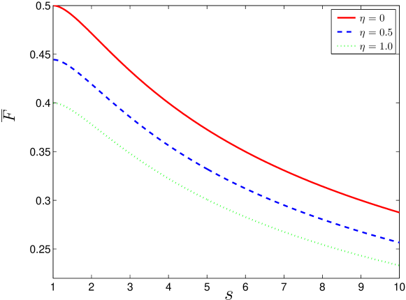
Figure 1: Fidelity benchmarks $\overline{F}(s,\eta)$ for measure-and-prepare schemes on ensembles with squeezing $s$, flatly distributed displacements and random phase space orientations, as a function of the squeezing $s$ (before additive noise is applied). The continuous (red) curve refers to pure states ($\eta=0$) while the dashed (blue) and dotted (green) curves refer to mixed states, for $\eta=0.5$ and $\eta=1$ respectively. Notice that, as one should expect, the pure state case is an upper bound for mixed states for the figure of merit $\overline{F}$. As stated in Theorem 3, the pure states case is also an upper bound for the Uhlmann fidelity benchmark of such mixed states.

This analytical result, though obtained for an ideal case, fully highlights the importance of radomising the input phase in practical instances. In fact, for a ‘flat’ distribution of displacements but fixed phase, the benchmark can be promptly inferred from the coherent states’ case, and is just $1/2\geq\sqrt{s}/(1+s)$, regardless of the degree of squeezing $s$ assumed. Randomising the input phase appears to be very helpful to provably reach the quantum regime in experiments (and, not surprisingly, the advantage granted by random rotations becomes more and more relevant with increasing squeezing): for pure states and degrees of squeezing within experimental reach ($s\lesssim 10$), the difference is around $0.2$ and might easily turn out to be crucial for experimental success. As we will see later on (see Sec. 5.3), and again not surprisingly, the same holds true for the randomisation of displacements.

4.2 Classical benchmark for mixed squeezed states under uniform rotations and displacements

Let us now consider the case of an input ensemble of mixed Gaussian states, derived from the initial pure states $\rho_{\omega}$, $\omega=(s,\xi,\theta)$ by the application of a noisy Gaussian channel $\mathcal{N}$, adding classical Gaussian noise with variance $\eta$, and thus acting on covariance matrices as $\gamma\mapsto\gamma+\eta\mathbbm{1}$ while leaving first moments invariant [21]. $\mathcal{N}$ can be understood as the application of random displacements to the input state, distributed according to a Gaussian with variance $\eta$. We will keep referring to $s$ as squeezing parameter (here, prior to the action of noise) and will refer to $\eta$ as to the ‘additive noise’.

As pointed out earlier we will use the overlap with $\rho_{\omega}$ as figure of merit:

$$F_{0}(s,\eta)=\sup_{T\in\mathcal{E}}\;\inf_{\xi,\theta}\;{\rm Tr}\,\left[T\Big{(}{\mathcal{N}}(\rho_{\omega})\Big{)}\rho_{\omega}\right]\,,$$

where, due to the symmetry (which is preserved by $\mathcal{N}$), one has again $F_{0}=\overline{F}$. For the same reason we can again restrict to phase space covariant channels and proceed along the lines of Theorem 1:

Theorem 2 (Benchmark—mixed states)

Let $\cal T$ be either the set of all measure-and-prepare schemes or the set of time-reversible channels. Within these sets the maximal achievable overlap for the teleportation or storage of mixed squeezed coherent states with squeezing $s$ and additive noise $\eta$ is given by

$$\overline{F}(s,\eta) = \sup_{T\in\cal T}\;\inf_{\xi,\theta}\;{\rm Tr}\,\left[T\Big{(}{\mathcal{N}}(\rho_{\omega})\Big{)}\rho_{\omega}\right]$$ (20)

$$= \left[\Big{(}1+\frac{\eta}{2}+\frac{1}{s}\Big{)}\Big{(}1+\frac{\eta}{2}+{s}\Big{)}\right]^{-1/2}\,.$$

Proof

As for Theorem 1, we restrict to phase space covariant channels $\tilde{T}$ parameterized by a density operator $\tau$ and obtain in an analogous way

$${\rm Tr}\,\left[\tilde{T}\Big{(}{\mathcal{N}}(\rho_{\omega})\Big{)}\rho_{\omega}\right]=\frac{1}{2\pi}\int{\rm d^{2}}\,\xi\;{\rm Tr}\left[\tau W_{\sqrt{2}\xi}\right]e^{-\frac{1}{2}\xi\cdot\Gamma\xi}=\frac{1}{2}{\rm Tr}\left[\tau\rho^{\prime}\right]\;,$$ (21)

where $\rho^{\prime}$ is now a centred Gaussian state with covariance matrix $\Gamma=\gamma_{\rho_{s}}+\eta/2$. Once again, the supremum over $\tau$ and thus over all time-reversible channels can be calculated by considering the state $\rho^{\prime}$ in the number basis, yielding

$$\sup_{\tau}\frac{1}{4\pi}{\rm Tr}\left[\left(\int_{0}^{2\pi}{\rm d}\theta U_{\theta}\rho^{\prime}U^{{\dagger}}_{\theta}\right)\tau\right] = \left|\left|\frac{1}{4\pi}\int_{0}^{2\pi}d\phi\;U_{\phi}\rho^{\prime}U_{\phi}^{\dagger}\right|\right|_{\infty}$$

$$=\ \max_{n}\frac{1}{2}\langle n|\rho^{\prime}|n\rangle = \frac{1}{2}\langle 0|\rho^{\prime}|0\rangle=\left[\Big{(}1+\frac{\eta}{2}+\frac{1}{s}\Big{)}\Big{(}1+\frac{\eta}{2}+{s}\Big{)}\right]^{-1/2},$$

which is Eq.(20) for time-reversible channels. Again, it can be shown by direct evaluation that the heterodyne strategy described by the map $H$ of Eq. (18) attains this bound, which completes the proof. $\square$

Notice that the overlap achieved by the ideal quantum channel (identity) is $\left[\Big{(}\frac{\eta}{2}+\frac{1}{s}\Big{)}\Big{(}\frac{\eta}{2}+{s}\Big{)}\right]^{-1/2}$. Also, $\overline{F}(s,0)=\overline{F}(s)$, as it should be since both the input ensemble and the figure of merit coincide with those of the preceding section in the noiseless case ($\eta=0$). Clearly, the optimal classical performance degrades with increasing noise (this is obviously the case for quantum strategies as well). Examples of such benchmarks for mixed states are displayed in Fig. 1.

For the same ensemble of mixed state, we shall also present a further analytical benchmark in the form of an upper bound, this time adopting the Uhlmann fidelity $f(T(\rho),\rho)$ as figure of merit:

Theorem 3 (Benchmark—mixed state fidelity)

Let $\cal T$ be either the set of all measure-and-prepare schemes or the set of time-reversible channels. Within these sets the maximal achievable worst case (or average) Uhlmann fidelity for the teleportation or storage of mixed squeezed coherent states with squeezing $s$ and arbitrary additive noise channel $\mathcal{N}$ is bounded as follows

$$\sup_{T\in{\cal E}}\inf_{\xi,\theta}f\big{(}T\left({\mathcal{N}}(\rho_{\omega})\right),{\mathcal{N}}(\rho_{\omega})\big{)}\leq\frac{\sqrt{s}}{1+s}\quad\forall\,\eta\in\mathbbm{R}\,.$$ (22)

Proof

Concavity of the fidelity allows us again to restrict to phase space covariant channels. All these channels commute with channels of the form ${\mathcal{N}}^{*}(W_{\xi})=W_{\xi}\exp[-||\xi||^{2}\eta/4]$ (${\mathcal{N}}^{*}$ standing for channel ${\mathcal{N}}$ in Heisenberg picture). The result follows then from the contractivity of cp-maps with respect to the fidelity, together with the pure state result of Theorem 1 [Eq.(11)]. $\square$

5 Quantum benchmarks derived by Semidefinite-Programming

5.1 Problem settings

So far, we treated input ensembles of squeezed states which are displaced in phase space according to a ‘flat’ distribution. Needless to say, this is an idealization as one cannot implement an arbitrarily large displacement in practice.

To be more realistic we have to treat an input ensemble of squeezed states whose first moments are essentially contained in a finite region of phase space, e.g., due to a sufficiently rapidly decaying probability distribution as in [8, 9].

This section will deal with this scenario by resorting to numerical means, as a purely analytical treatment appears to be far too involved for finite, non-flat distributions of displacements (where the restrictions to phase space covariant channels is no longer optimal). We will show that the problem of computing benchmarks of the desired kind can be cast into a semidefinite program (SDP). As such, it comes with a guarantee of computing the correct value, as SDPs come in pairs of a primal and a dual problem which yield converging upper and lower bounds to the sought solution [30]. As the original SDP is in an infinite dimensional space, truncation will be necessary and will induce errors. However, we will provide a rigorous bound to the truncation errors so that the finally derived benchmarks are reliable and rigorous, constituting upper bounds to the actual optimal classical figures of merit.

The figure of merit we use is again the average overlap

$$\overline{F}=\sup_{T\in\mathcal{E}}\int d\omega\;q(\omega){\rm Tr}\left[T\Big{(}{\mathcal{N}}(\rho_{\omega})\Big{)}\rho_{\omega}\right],$$

where $\mathcal{N}$ is a noisy channel that describes the noise suffered by $\rho_{\omega}$ before entering the storage or teleportation device, which for our purposes should be

1. a channel which allows for the computation of the matrix elements in the Fock basis $\langle k|{\mathcal{N}}(\rho_{\omega})|l\rangle$, e.g., a Gaussian channel [21]

2. rotationally covariant, i.e., $\mathcal{N}\left(U_{\theta}\rho U_{\theta}^{\dagger}\right)=U_{\theta}\mathcal{N}\left(\rho\right)U_{\theta}^{\dagger}$ for all $\rho,\theta$.

Fortunately, channels representing attenuation, amplification, and thermal noise are all of this type, the attenuation channel being probably the most relevant here, as it models losses of photons/excitations which are the dominant decoherence process in the practical realisations we have in mind, involving traveling waves of light. Thus we will adopt it in the following, denoting it by $\mathcal{N}_{\lambda}$. The parameter $\lambda\in[0,1]$ represents the transmitivity (in intensity) such that the channel acts on, respectively, covariant matrix $\gamma_{\rho}$ and vector of first moments $d_{\rho}$ as: $\gamma_{\rho}\mapsto\lambda\gamma_{\rho}+(1-\lambda)\mathbbm{1}$ and $d_{\rho}\mapsto\sqrt{\lambda}d_{\rho}$. Another crucial assumption for our method is that the input distribution $q$ is uniform in the angle $\theta$. Moreover, we will consider ensembles with constant degree of squeezing $s$ (although this is not necessary for the method). Hence $q$ can be considered a probability distribution which depends only on the displacement $\xi$ and therefore

$$\overline{F}=\sup_{T\in\mathcal{E}}\int_{\theta\in[0,2\pi]}\int_{\xi\in\mathbb{R}^{2}}q(\xi){\rm Tr}\,\left[T\Big{(}\mathcal{N}_{\lambda}(U_{\theta}\rho_{s,\xi}U_{\theta}^{\dagger})\Big{)}\Big{(}U_{\theta}\rho_{s,\xi}U_{\theta}^{\dagger}\Big{)}\right]\frac{d\theta}{2\pi}d\xi,$$ (23)

where $\rho_{s,\xi}$ is a pure squeezed states with degree of squeezing $s$ and displacement $\xi$. Note that $\overline{F}$ in this way becomes a functional of $\lambda,s$ and of the distribution $q$.

5.2 Reduction to a finite dimensional semidefinite program

In this subsection, we will see how we can reduce the quantum benchmark $\overline{F}$ in Eq.(23) to a finite dimensional SDP. We first show that Eq.(23) can be reduced to an infinite dimensional SDP problem. To this end, we use a simple correspondence between the set of all entanglement breaking channels and the set of bipartite separable positive operators [31] which is nothing but the Choi-Jamiolkowski isomorphism [32], albeit for an infinite dimensional system (see B for a proof):

Theorem 4 (Choi-Jamiolkowski)

Suppose $\mathfrak{B}(\mathcal{H})$ is the space of all bounded operators and $\mathfrak{C}_{1}(\mathcal{H})$ is the space of all trace class operators on a separable Hilbert space $\mathcal{H}$. Then, for all entanglement breaking channels $\Psi$ on $\mathcal{H}$, there exist a unique separable positive bounded operator $\Omega(\Psi)$ on $\mathcal{H}\otimes\mathcal{H}$ such that $Tr_{B}(\Omega(\Psi))=\mathbbm{1}_{A}$ and

$$\Tr(B\Psi(A))=\Tr(\Omega(\Psi)A\otimes B)$$ (24)

for all $A\in\mathfrak{C}_{1}(\mathcal{H})$ and $B\in\mathfrak{B}(\mathcal{H})$. Conversely, for a separable positive bounded operator $\Omega$ on $\mathcal{H}\otimes\mathcal{H}$ satisfying $Tr_{B}(\Omega)=\mathbbm{1}_{A}$, there exists a unique channel $\Psi(\Omega)$ such that it is entanglement breaking and satisfies Eq.(24).

By means of the above theorem, we immediately derive an upper bound to the quantity $\overline{F}$ of Eq.(23) in an infinite dimensional SDP form by enlarging the set of positive separable operators (denoted by ${\rm Sep}$) to the set of positive operators with positive partial transpose (PPT) $\Omega^{\Gamma}\geq 0$:

$$\overline{F} = \sup_{\Omega\in\mathfrak{B}(\mathcal{H}\otimes\mathcal{H})}\left\{\Tr(\Omega\eta)\Big{|}\Omega\in{\rm Sep},\Tr_{B}\Omega=\mathbbm{1}_{A}\right\}$$ (25)

$$\leq \sup_{\Omega\in\mathfrak{B}(\mathcal{H}\otimes\mathcal{H})}\left\{\Tr(\Omega\eta)\Big{|}\Omega\geq 0,\Omega^{\Gamma}\geq 0,\Tr_{B}\Omega=\mathbbm{1}_{A}\right\}.$$

In the above equations $\eta$ is a state on $\mathcal{H}\otimes\mathcal{H}$ defined by

$$\eta\stackrel{{\scriptstyle\rm def}}{{=}}\int_{\theta\in[0,2\pi]}\int_{\xi\in\mathbb{R}^{2}}q(\xi)\ U_{\theta}{\mathcal{N}}_{\lambda}(\rho_{s,\xi})U_{\theta}^{\dagger}\otimes\left(U_{\theta}\rho_{s,\xi}U_{\theta}^{\dagger}\right)\frac{d\theta}{2\pi}\;d\xi,$$ (26)

where we exploited the rotational covariance of $\mathcal{N}_{\lambda}$.

Here, we should remark that, if $\lambda=1$ and $q(\xi)=\frac{\alpha}{\pi}\exp[-\alpha||\xi||^{2}]$ for $\alpha\geq 0$, the inequality in Eq.(25) is actually an equality. This is because, under such assumptions, we can choose an optimal $\Omega$ to be Gaussian [9] and the PPT condition $\Omega^{\Gamma}\geq 0$ is necessary and sufficient for a two-mode Gaussian state $\Omega$ to be separable [33, 34].

In the remaining part of this subsection we will transform the above infinite dimensional SDP into a finite dimensional SDP. We will need the following statement:

Lemma 1 (Operator norm bound)

If a positive separable operator $\Omega\in\mathfrak{B}(\mathcal{H}\otimes\mathcal{H})$ satisfies $\Tr_{B}\Omega=\mathbbm{1}_{A}$, then, $\Omega$ also satisfies $\|\Omega\|_{\infty}\leq 1$, where $\|\cdot\|_{\infty}$ is the operator norm.

Proof

From the proof of Theorem 4, $\Omega$ can be written as $\Omega(\Psi)=\int_{\cal X}M(dx)\otimes\sigma(x)$ by using a POVM $\{M(dx)\}$ and a set of states $\{\sigma(x)\}$. Then, for any normalized state $\left|\Phi\right\rangle$ on $\mathcal{H}\otimes\mathcal{H}$, we can bound $\left\langle\Phi\right|\Omega\left|\Phi\right\rangle$ as follows:

$$\left\langle\Phi\right|\Omega\left|\Phi\right\rangle = \int_{\cal X}\Tr(M(dx)\otimes\sigma(x)\left|\Phi\right\rangle\left\langle\Phi\right|)$$

$$\leq \int_{\cal X}\Tr(M(dx)\rho_{A})=1,$$

where $\rho_{A}$ is defined as $\Tr_{B}(\left|\Phi\right\rangle\left\langle\Phi\right|)$ and we used that $\sigma(x)\leq\mathbbm{1}$ together with $M({\cal X})=\mathbbm{1}$. Therefore, we have $\|\Omega\|_{\infty}=\sup_{\Phi}\left\langle\Phi\right|\Omega\left|\Phi\right\rangle\leq 1$. $\square$

Notice that, even if $\|\Omega\|_{\infty}\leq 1$ was shown for the corresponding operator of an entanglement breaking channel, this fact may not be true for other channels (in general we can only show that the geometric measure [35] $G(\Omega(T))\stackrel{{\scriptstyle\rm def}}{{=}}\sup_{\sigma\in Sep}\Tr\left(\Omega(T)\sigma\right)\leq 1$).

Before we derive a finite SDP problem from Eq.(25), we observe the following crucial fact: By means of the action of the group integral over $\{U_{\theta}\otimes U_{\theta}\}_{\theta\in[0,2\pi]}$, $\eta$ is block diagonalized as

$$\eta=\sum_{c=0}^{\infty}Q_{c}\left[\int_{\xi\in\mathbb{R}^{2}}q(\xi)\ \mathcal{N}_{\lambda}(\rho_{s,\xi})\otimes\rho_{s,\xi}\;d\xi\right]Q_{c},$$ (27)

where $Q_{c}\stackrel{{\scriptstyle\rm def}}{{=}}\sum_{k+l=c}\left|k\right\rangle\left\langle k\right|\otimes\left|l\right\rangle\left\langle l\right|$ is a finite dimensional projector. Thus, defining $P_{c}\stackrel{{\scriptstyle\rm def}}{{=}}\sum_{i=0}^{c}Q_{i}$, we obtain $\eta-P_{c}\eta P_{c}=\sum_{i=c+1}^{\infty}Q_{i}\eta Q_{i}\geq 0$ for all $c$. We arrive at the finite SDP upper bound now as follows: Suppose a separable positive $\Omega$ satisfies $\Tr_{B}\Omega=\mathbbm{1}_{A}$. Then,

$$\Tr(\Omega\eta) = \Tr(\Omega P_{c}\eta P_{c})+\Tr(\Omega(\eta-P_{c}\eta P_{c}))$$ (28)

$$\leq \Tr(\Omega P_{c}\eta P_{c})+\|\Omega\|_{\infty}\Tr\big{(}\eta-P_{c}\eta P_{c}\big{)}$$

$$\leq \Tr(\Omega P_{c}\eta P_{c})+\Tr(\eta-P_{c}\eta P_{c})$$

$$= \Tr(\Omega P_{c}\eta P_{c})-\Tr(P_{c}\eta P_{c})+1,$$

where we used the positivity of $\eta-P_{c}\eta P_{c}$ and Lemma 1.

Finally, by means of Eq.(28), we can derive an upper bound to the first line of Eq.(25). Denoting with $R_{c}=\left(\sum_{i=0}^{c}\left|i\right\rangle\left\langle i\right|\right)\otimes\left(\sum_{i=0}^{c}\left|i\right\rangle\left\langle i\right|\right)$ the projection onto the subspace with a photon number smaller than $c$ in each mode, with support ${\rm supp}R_{c}$, we obtain

$$\overline{F} \leq \sup_{\Omega\in\mathfrak{B}\left(\mathcal{H}\right)}\left\{\Tr(\Omega P_{c}\eta P_{c})\Big{|}\Omega\in{\rm Sep},\Tr_{B}\Omega=\mathbbm{1}_{A}\right\}+1-\Tr(P_{c}\eta P_{c})$$ (29)

$$= \sup_{\Omega\in\mathfrak{B}\left(\mathcal{H}\right)}\left\{\Tr(R_{c}\Omega R_{c}P_{c}\eta P_{c})\Big{|}\Omega\in{\rm Sep},\Tr_{B}\Omega=\mathbbm{1}_{A}\right\}+1-\Tr(P_{c}\eta P_{c})$$

$$\leq \sup_{\Omega\in\mathfrak{B}\left({\rm supp}R_{c}\right)}\left\{\Tr(\Omega P_{c}\eta P_{c})\Big{|}\Omega\in{\rm Sep},\Tr_{B}\Omega\leq\mathbbm{1}_{A}\right\}+1-\Tr(P_{c}\eta P_{c})$$

$$\leq \sup_{\Omega\in\mathfrak{B}\left({\rm supp}R_{c}\right)}\left\{\Tr(\Omega P_{c}\eta P_{c})\Big{|}\Omega\geq 0,\Omega^{\Gamma}\geq 0,\Tr_{B}\Omega\leq\mathbbm{1}_{A}\right\}+1-\Tr(P_{c}\eta P_{c}),$$

The above upper bound now only involves a finite dimensional SDP, as the original infinite dimensional $\Omega$ has been replaced by the finite dimensional $R_{c}\Omega R_{c}$, with the same type of constraints (note that $R_{c}$ was introduced to preserve the separability of the operator). Similarly, the term $\Tr(P_{c}\eta P_{c})$ is just a trace of a finite dimensional matrix, so that we can numerically compute every term of the last formula of Eq.(29) for as large a truncation parameter $c$ as our computer allows. Thus, Eq.(29) enables us to efficiently calculate an upper bound for the quantum benchmark $\overline{F}$ for any probability density $q(\xi)$, that is, ultimately, for any rotationally-invariant input ensemble. Moreover, since in the limit of large $c$ we obtain the second formula of Eq.(25), we can expect that this upper bound reaches the exact value for this bound for sufficiently large $c$. Finally, we rephrase Eq.(29) in the form of a theorem:

Theorem 5 (Benchmark—SDP)

With the above definitions, for any probability density $q(\xi)$ on $\mathbb{R}^{2}$ and rotationally covariant noise channel $\mathcal{N}$, we have

$$\overline{F}\leq\sup_{\Omega\in\mathfrak{B}\left({\rm supp}R_{c}\right)}\left\{\Tr(\Omega P_{c}\eta P_{c})\Big{|}\Omega\geq 0,\Omega^{\Gamma}\geq 0,\Tr_{B}\Omega\leq\mathbbm{1}_{A}\right\}\quad+1-\Tr(P_{c}\eta P_{c})\,.$$

(30)

5.3 Results of numerical calculations

In this subsection, we present results of numerical calculations which were produced using inequality (5). In order to reduce the memory requirements, we further exploit the block diagonal structure of $\eta$ in Eq.(27) and impose $\sum_{j=0}^{2c}Q_{j}\Omega Q_{j}=\Omega$ for the implementation. The evaluation of the bound then splits into two terms:

$$\overline{F}_{finite}\stackrel{{\scriptstyle\rm def}}{{=}}\sup_{\Omega\in\mathfrak{B}\left({\rm supp}R_{c}\right)}\left\{\Tr(\Omega P_{c}\eta P_{c})\Big{|}\Omega\geq 0,\Omega^{\Gamma}\geq 0,\Tr_{B}\Omega\leq\mathbbm{1}_{A}\right\},$$

$$\epsilon_{error}\stackrel{{\scriptstyle\rm def}}{{=}}1-\Tr(P_{c}\eta P_{c}).$$

Denoting the r.h.s. of (5) by $\overline{F}_{infinite}$ we have

$$\overline{F}_{infinite}=\overline{F}_{finite}+\epsilon_{error}.$$ (31)

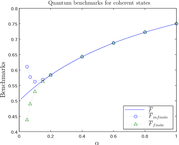
Figure 2: A plot of the known optimal classical bound $\overline{F}=\frac{2\alpha+1}{2(\alpha+1)}$, the upper bound $\overline{F}_{infinite}$ derived by our numerical calculation with $c=35$, and the result of the finite SDP $\overline{F}_{finite}$ (without corrected truncation error) for an ensemble of coherent states, no noise $(\lambda=1)$, and $q(\xi)=\frac{\alpha}{\pi}\exp[-\alpha||\xi||^{2}]$.

Our computation proceeds along the following steps:

1. Compute matrix elements of $\left\langle k_{1}\right|{\mathcal{N}}_{\lambda}(\rho_{s,\xi})\left|l_{1}\right\rangle$ and $\left\langle k_{2}\right|\rho_{s,\xi}\left|\l_{2}\right\rangle$ for all $k_{1}$, $k_{2}$, $l_{1}$, $l_{2}$ satisfying $k_{1}+k_{2}\leq c$ and $l_{1}+l_{2}\leq c$; $c$ is a fixed maximum photon number practically bounded by the computer memory. For the calculation, we used an analytical formula for matrix elements of single-mode Gaussian states as a finite sum over Hermite polynomials (see Eq.(4.10) of [36]).

2. Evaluate the following integral over $\xi$

   $$\int_{\xi\in\mathbb{R}^{2}}q(\xi)\left\langle k_{1}\right|\mathcal{N}_{\lambda}(\rho_{s,\xi})\left|l_{1}\right\rangle\left\langle k_{2}\right|\rho_{s,\xi}\left|l_{2}\right\rangle\;d\xi$$

   by Quasi-Monte Carlo with the Halton sequence [37].

3. From Eq.(27), we derive $P_{c}\eta P_{c}$.

4. Finally, we solve the SDP leading to $\overline{F}_{infinite}$.

Here, all the above numerical calculations were implemented in Matlab, and the SDP is solved using the Matlab toolbox SeDuMi version 1.1 [38]. In the above numerical calculation, we do not use any approximation except for the Quasi-Monte Carlo integral.

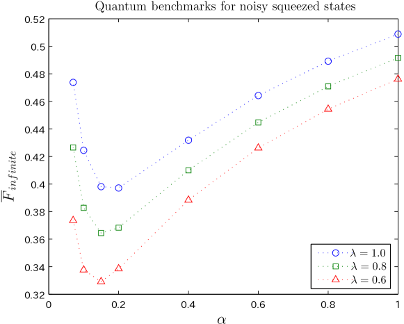
Figure 3: Results of numerical calculations of the quantum benchmark $\overline{F}_{infinite}$ for an ensemble of noisy squeezed states displaced according to a Gaussian probability distribution $q(\xi)=\frac{\alpha}{\pi}\exp[-\alpha||\xi||^{2}]$. Levels used in Fock space $c=30$, squeezing $s=8$, and losses $(1-\lambda)=0.4,0.2,0$.

As a first application, in order to provide the reader with a convincing test for our numerical calculations, we show that our method reproduces the result of the optimal quantum benchmark for displaced coherent states derived in [9]. Suppose $\lambda=s=1$ and the input ensemble is distributed according to $q(\xi)=\frac{\alpha}{\pi}\exp[-\alpha||\xi||^{2}]$. That is we deal with an ensemble of coherent states whose centers are distributed according to a Gaussian distribution with variance $1/(2\alpha)$. Hence, using the invariance of the ensemble under rotations we obtain

$$\eta=\int_{\xi\in\mathbb{R}^{2}}\frac{\alpha}{\pi}\exp[-\alpha||\xi||^{2}]\ \rho_{1,\xi}\otimes\rho_{1,\xi}\;d\xi\;.$$ (32)

The quantum benchmark $\overline{F}$ in this case was shown [9] to be (note that our definition of the parameter $\alpha$ is different by the factor $2$ from the definition in [9])

$$\overline{F}=\frac{2\alpha+1}{2(\alpha+1)}.$$ (33)

So we can compare our upper bound $\overline{F}_{infinite}$ derived by SDP with the optimal bound, which is shown in Figure 2 for the maximum photon number $c=35$. As expected the numerics satisfies $\overline{F}_{infinite}>\overline{F}>\overline{F}_{finite}$ but we observe in Fig. 2 that as long as $\alpha\geq 0.2$, the values of both $\overline{F}_{infinite}$ and $\overline{F}_{finite}$ are essentially indistinguishable from the optimal bound $\overline{F}$ while for $\alpha\leq 0.2$ we find noticeable differences. In other words, in Eq.(31) the term $\epsilon_{error}$, which originates from the truncation of the dimension, becomes dominant in this region. As a result, the minimum value of $\overline{F}_{infinite}$ is around $\alpha=0.15$, i.e., $\overline{F}_{infinite}$ is not monotonically decreasing with respect to $\alpha$.

From this result, we may expect that our upper bounds are also almost optimal in other situations (different $q,s,\mathcal{N}$) as long as $\epsilon_{error}$ is small with respect to $\overline{F_{finite}}$.

Next, we consider the case of an ensemble of noisy squeezed states with a fixed squeezing parameter $s$ and again a Gaussian prior distribution for $\xi$. We show the results of our calculation in Figure 3. Here, we chose $c=30$, $s=8$, and plot for $\lambda=0.6,0.8,1$. In this figure, we can observe that, as expected, $\overline{F}_{infinite}$ decreases with decreasing $\lambda$. Due to the increasing contribution of $\epsilon_{error}$ for decreasing $\alpha$, the best (lowest) values of our benchmarks are achieved, under realistic losses, for $\alpha\simeq 0.15$. This value, though maybe non-optimal, is suitable for comparisons with realistic experimental situations. A simple, preliminary analysis of possible experimental noise conditions indicates that the values of the benchmark for such parameters could be beaten by forthcoming experiments aimed at the teleportation or storage of squeezed states. Let us mention that single states have already been teleported or stored, both with light modes [15, 16] and with atomic memories [17, 18]. The experimental demonstration of the transmission of a full ensembles of squeezed states is yet to come, but techniques are ripe for it to be realized in both settings: our method is ready for the analysis of such developments by direct comparison.

Finally, we consider the simple case of an ensemble of randomly rotated squeezed vacuum states without displacement in phase space. That is, we choose $q(\xi)=\delta(||\xi||^{2})$, shown in Figure 4.

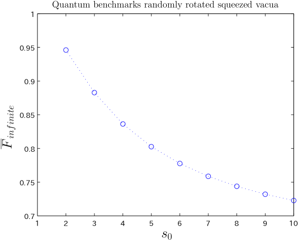
Figure 4: The results for the quantum benchmark $\overline{F}_{infinite}$ for an ensemble of randomly rotated squeezed vacuum states without displacement, i.e., $q(\xi)=\delta(||\xi||^{2})$, $c=30$ and no noise ($\lambda=1$).

Here, we chose $c=30$ and plot for $2\leq s\leq 10$. Note that for $s=1$ there is only one state in the ensemble, the vacuum state, so that $\overline{F}=1$ in this case. Fig. 4 clearly shows that, if the displacements in phase space are not randomised, the classical benchmarks we derived increase significantly and and beating them in current experiments would be a daunting challenge: distributing the displacements of the input ensemble is thus definitely, at present, a technical necessity in order to achieve a certifiable quantum performance [39].

6 Summary and Conclusions

In this work we have derived upper bounds on the performance of classical ’measure and prepare’ protocols for the quantum storage and teleportation of ensembles of squeezed states of continuous variable systems. These bounds may be employed as benchmarks to discern truly quantum mechanical performances in experiments aimed at the realization of such processes. Motivated by currently available experimental capabilities and concrete set-ups, we have considered ensembles comprised of states with fixed squeezing, but allowed for the possibility of random rotations and translations of those states in phase space.

Fully analytical benchmarks have been obtained for pure squeezed states as well as mixed states obtained from the application of additive thermal noise, for the case of completely unknown rotations and translations in phase space. In these ideal cases, the benchmarks decrease monotonically with increasing degree of squeezing $s$, vanishing for diverging $s$: in this sense, increasing the squeezing reveals the infinite dimensional character of the Hilbert space. Furthermore, we have presented a numerical technique that first reduces the problem to a finite dimensional setting with rigorous error bounds, and then allows for the numerical solution of the remaining finite dimensional problem using semi-definite programming. The so obtained bounds are rigorous and this approach may be applied to more general settings, even beyond the Gaussian regime, for variable squeezing and arbitrarily distributed displacements, with the only proviso that the distribution over rotations should be still rotationally symmetric in phase space, to maintain covariance under rotations (which was essential in deriving rigorous bounds for the truncated problem). Let us also emphasise that our numerical strategy can be reliably applied to finite sets of states as well (rather than to continuous distributions), which are what, strictly speaking, is sampled in actual experiments.

Our numerical results strongly indicate that allowing for randomised displacements is crucial to outperform optimal classical strategies with current quantum technologies and that, on the other hand, if such a randomisation is allowed, realistic setups might be able to enter the quantum regime with squeezed states. Likewise, randomised phases, other than providing a much more “appealing” evidence for the teleportation or storage of the states (since, in such a case, states with a varying structure of second moments would be transmitted), seems to be needed for the benchmarks to be beaten.

Overall, the results presented here will provide a useful resource for assessing the quantum mechanical character of experiments aimed at demonstrating quantum storage and transmission of squeezed states. In a future work, these methods will be applied to concrete experiments.

Note added. We acknowledge that, very recently (after the completion of this study and during the writing of the present paper), another work appeared (Ref. [12]) where benchmarks based on the Uhlmann fidelity for rotationally covariant ensembles were studied, and the reduction of the benchmark estimation to an SDP was independently derived.

Appendix A Phase space covariant channels

In this appendix, we collect useful results about ‘phase space covariant’ channels, i.e. channels covariant under the action of the Weyl-Heisenberg group of displacement operators $\{W_{\xi},\xi\in{\mathbb{R}}^{2n}\}$. For a phase space covariant channel one has

$$T(W_{\xi}^{{\dagger}}\hat{O}W_{\xi})=W_{\xi}^{{\dagger}}T(\hat{O})W_{\xi}\,,\quad\forall\,\hat{O}\in{\mathfrak{B}}(L_{2}({\mathbb{R}})^{\otimes n})\quad{\rm and}\quad\forall\,\xi\in\mathbb{R}^{2n}\,.$$

[${\mathfrak{B}}(L_{2}({\mathbb{R}})^{\otimes n})$ being the set of bounded linear operators on $n$ copies of the bosonic Hilbert space]. These results were already used (though not explicitly detailed) in [25, 26]. Central to this analysis is the characterization of the class of “linear bosonic channels” in terms of their action on Weyl operators, given in [40], which we report here without proof in the form of the following lemma. Recall that $T^{*}$ stands for the operation $T$ in the Heisenberg picture.

Lemma 2 (Linear bosonic channels)

A map $T^{*}(W_{\xi}):=f(\xi)W_{X\xi}$ is a quantum channel if and only if $f$ is the quantum characteristic function with respect to a modified symplectic form $\tilde{\sigma}:=\sigma-X^{T}\sigma X$. That is, $f:\mathbb{R}^{2n}\rightarrow\mathbb{C}$ has to be continuous, $f(0)=1$ and every matrix with entries

$$M_{kl}=f\big{(}\xi^{(k)}-\xi^{(l)}\big{)}\exp{\Big{[}\frac{i}{2}\xi^{(k)}\cdot\tilde{\sigma}\xi^{(l)}\Big{]}}$$ (34)

has to be positive semi-definite for all $\xi^{(k)},\xi^{(l)}\in\mathbb{R}^{2n}$.

Note that condition (34) for $\tilde{\sigma}=\sigma$ ($\tilde{\sigma}=0$) is equivalent to $f$ being a quantum (classical) characteristic function.

The following characterization of phase space covariance ensues:

Lemma 3 (Phase space covariant channels)

Every phase space covariant channel is uniquely characterized by a classical characteristic function $f$ and acts in the Heisenberg picture as

$$T^{*}(W_{\xi})=f(\xi)W_{\xi}.$$ (35)

Proof

Consider the action of $T^{*}$ on a Weyl operator $W_{\xi}$. Exploiting the Weyl relations, phase space covariance (with respect to any $W_{\eta}$) leads to

$$W_{\eta}T^{*}(W_{\xi})=e^{i\xi\cdot\sigma\eta}\;T^{*}(W_{\xi})W_{\eta}\,.$$ (36)

It is straightforward to check that this entails

$$\big{[}T^{*}(W_{\xi})W_{\xi}^{\dagger},W_{\eta}\big{]}=0\,,\quad\forall\,\xi,\eta\in\mathbbm{R}^{2n}\,.$$ (37)

The irreducibility of the Weyl system then implies $T^{*}(W_{\xi})W_{\xi}^{\dagger}\propto\mathbbm{1}$. Denoting the proportionality constant by $f(\xi)$, we have a map of the form in Lemma 2 with $X=\mathbbm{1}$. Hence, $f$ has to be a classical characteristic function. $\square$

Let us denote by $\vartheta$ the time reversal (or matrix transposition) operator. Every entanglement breaking channel, i.e., ‘measure-and-prepare scheme’ (see Ref. [23]), is such that $T\circ\vartheta$ is completely positive (that is, the Choi matrix – or the Jamiolkowski state – has positive partial transpose). Moreover, time reversal acts very simply in phase space by flipping the sign of one of the two canonical quadratures (see, e.g., [33]): $\vartheta(W_{\xi})=W_{Z\xi}$, where $Z=\oplus_{j=1}^{n}\sigma_{z}$ ($\sigma_{z}$ being the Pauli $z$ matrix). We will now apply this additional constraint to phase space covariant channels, in order to achieve a stronger characterization:

Lemma 4 (Time-reversible channels)

A phase space covariant channel $T$ is such that $T\circ\vartheta$ is completely positive iff it has the form

$$T^{*}(W_{\xi})=f\big{(}\xi/\sqrt{2}\big{)}W_{\xi},$$ (38)

where $f$ is any quantum characteristic function, i.e., there is a density operator $\tau\in{\mathfrak{C}}_{1}(L_{2}(\mathbbm{R})^{\otimes n})$ such that $f(\xi)=\Tr{\left[\tau W_{\xi}\right]}$.

Proof

Using Lemma 3 we obtain

$$\vartheta\circ T^{*}(W_{\xi})=f(\xi)\vartheta(W_{\xi})=f(\xi)W_{Z\xi}\,,$$ (39)

where $Z$ reverses the momenta so that $Z^{T}\sigma Z=-\sigma$. Following Lemma 2 this map is completely positive if and only if positivity of Eq. (34) holds for $\tilde{\sigma}=2\sigma$. The result follows then by substituting $\xi\rightarrow\xi/\sqrt{2}$. $\square$

Appendix B Proof of Theorem 4

Proof

Suppose $\Psi$ is a entanglement breaking channel and can be written [23, 22] as $\Psi(\rho)=\int_{\cal X}\Tr(M(dx)\rho)\sigma(x)$ for all $\rho\in\mathfrak{C}_{1}(\mathcal{H})$, where $\sigma(x)\in\mathfrak{C}_{1}(\mathcal{H})$ are states and $M$ is a POVM, i.e., $M(X)\geq 0$ for all Borel subsets $X$ of a complete separable metric space $\cal X$ for which $M({\cal X})=\mathbbm{1}$.

Then, $\Omega(\Psi)=\int_{\cal X}M(dx)\otimes\sigma(x)$ satisfies $Tr_{B}(\Omega(\Psi))=\mathbbm{1}_{A}$ and Eq.(24). Moreover, suppose there exists a $\Omega^{\prime}(\Psi)$ satisfying $Tr_{B}(\Omega^{\prime}(\Psi))=\mathbbm{1}_{A}$ and Eq.(24). Then, since $\Tr(\Omega^{\prime}(\Psi)\left|i\right\rangle\left\langle j\right|\otimes\left|k\right\rangle\left\langle l\right|)=\Tr(\left|k\right\rangle\left\langle l\right|\Psi(\left|i\right\rangle\left\langle j\right|))=\Tr(\Omega(\Psi)\left|i\right\rangle\left\langle j\right|\otimes\left|k\right\rangle\left\langle l\right|)$ for a orthonormal basis $\{\left|i\right\rangle\}_{i}$ of $\mathcal{H}$, we immediately have $\Omega^{\prime}=\Omega$.

Conversely, suppose there exists a separable positive bounded operator $\Omega$ on $\mathcal{H}\otimes\mathcal{H}$ satisfying $Tr_{B}(\Omega)=\mathbbm{1}_{A}$ and can be written as $\Omega=\int|\Phi\rangle\langle\Phi|\otimes|\varphi\rangle\langle\varphi|\;\mu(d\Phi d\varphi)$ with measure $\mu$. We define a channel $\Psi$ as $\rho\mapsto\int\Tr(M(d\varphi)\rho)|\varphi\rangle\langle\varphi|$, where $M(d\varphi)\stackrel{{\scriptstyle\rm def}}{{=}}\int_{\Phi}|\Phi\rangle\langle\Phi|\mu(d\Phi d\varphi)$. Then, since $Tr_{B}(\Omega)=\mathbbm{1}_{A}$, $M$ is a POVM; that is, $\Psi$ is an entanglement breaking channel. Evidently, $\Psi$ satisfies Eq.(24). Moreover, suppose an entanglement breaking channel $\Psi^{\prime}$ also satisfies Eq. (24). Then, since $\Tr(B\Psi^{\prime}(A))=\Tr(\Omega(\Psi)A\otimes B)=\Tr(B\Psi(A))$ for all $B\in\mathfrak{B}(\mathcal{H})$, $\Psi^{\prime}(A)=\Psi(A)$ for all $A\in\mathfrak{C}_{1}(\mathcal{H})$. $\square$

References

References

- [1] Furusawa A, Sørensen J L, Braunstein S L, Fuchs C A, Kimble H J and Polzik E S 1998 Science 282, 706
- [2] Yonezawa H, Aoki T and Furusawa A, Nature 431 430
- [3] Zhang T C, Goh K W, Chou C W, Lodahl P and Kimble H J 2003 Phys. Rev. A 67 033802
- [4] Schori C, Julsgaard B, Sørensen J L and Polzik E S 2002 Phys. Rev. Lett. 89 057903 (2002)
- [5] Sherson J F, Krauter H, Olsson R K, Julsgaard B, Hammerer K, Cirac I and Polzik E S 2006 Nature 443, 557
- [6] Riebe M, Häffner H, Roos C F, Hänsel W, Benhelm J, Lancaster G P T, Körber T W, Becher C, Schmidt-Kaler F, James D F V and Blatt R 2004 Nature 429 734
- [7] Barrett M D, Chiaverini J, Schaetz T, Britton J, Itano W M, Jost J D, Knill E, Langer C, Leibfried D, Ozeri R and Wineland D J 2004 Nature 429 737
- [8] Braunstein S L, Fuchs C A and Kimble H J 2000 J. Mod. Optics 47 267
- [9] Hammerer K, Wolf M M, Polzik E S, Cirac J I 2005 Phys. Rev. Lett. 94 150503
- [10] Serafini A, Dahlsten O C O and Plenio M B 2007 Phys. Rev. Lett. 98 170501
- [11] Adesso G and Chiribella G 2008 Phys. Rev. Lett. 100 170503
- [12] Calsamiglia J, Aspachs M, Muñoz-Tapia R and Bagan E 2008 Preprint arXiv:0807.5126
- [13] Werner R F 1998 Phys. Rev. A 58 1827
- [14] Horodecki P, Horodecki M and Horodecki R 1999 Phys. Rev. A 60 1888
- [15] Takei N, Aoki T, Koike S, Yoshino K, Wakui K, Yonezawa H, Hiraoka T, Mizuno J, Takeoka M, Ban M and Furusawa A 2005 Phys. Rev. A 72 042304
- [16] Yonezawa H, Braunstein S L and Furusawa A 2007 Phys. Rev. Lett. 99 110503
- [17] Appel J, Figueroa E, Korystov D, Lobino M and Lvovsky A I 2008 Phys. Rev. Lett. 100 093602;
- [18] Honda K, Akamatsu D, Arikawa M, Yokoi Y, Akiba K, Nagatsuka S, Tanimura T, Furusawa A and Kozuma M 2008 Phys. Rev. Lett. 100 093601
- [19] Eisert J and Plenio M B 2003 Int. J. Quant. Inf. 1 479
- [20] Holevo A S 1982 Probabilistic and statistical aspects of quantum theory (Amsterdam: North-Holland Publishing Company)
-
[21]
Eisert J and Wolf M M 2007 Gaussian Quantum Channels Quantum Information with Continuous
Variables of Atoms and Light G Leuchs, N Cerf and E S Polzik (London: Imperial
College Press)
(Eisert J and Wolf M M 2005 Preprint quant-ph/0505151) - [22] Holevo A S, Shirokov M E and Werner R F 2005 Russian Math. Surveys 60 N2
- [23] Holevo A S 2008 Preprint arXiv:0802.0235
- [24] Uhlmann A 1976 Rep. Math. Phys. 9 273
- [25] Cerf N J, Krueger O, Navez P, Werner R F and Wolf M M 2005 Phys. Rev. Lett. 95 070501
- [26] Krueger O 2007 Quantum Information Theory with Gaussian Systems PhD thesis (Technical University, Braunschweig)
- [27] Werner R F 2004 The Uncertainty Relation for Joint Measurement of Position and Momentum Quantum Information, Statistics, Probability O Hirota (Paramus, NJ: Rinton Press) p 153
- [28] An alternative way of noting that this bound remains the same when restricting to measure-and-prepare schemes is to realize that (i) (a Gaussian!) yields the maximum in Eq.(17) and (ii) for two-mode Gaussian states (bearing in mind the Choi-matrix of ) the PPT-criterion is necessary and sufficient for separability.
- [29] Scutaru H 1998 J. Math. Phys. 39 6403
- [30] Boyd S and Vandenberghe L 2004 Convex Optimization (Cambridge: Cambridge University Press)
- [31] Rains E 2001 IEEE Trans. on Inf. Theor. 47 2921
- [32] Jamiolkowski A 1972 Rep. Math. Phys. 3 275; Choi M-D 1975 Lin. Alg. Appl. 10 285
- [33] Simon R 2000 Phys. Rev. Lett. 84 2726
- [34] Werner R F and Wolf M M 2001 Phys. Rev. Lett. 86 3658
- [35] Plenio M B and Virmani S 2007 Quant. Inf. Comp. 7 1
- [36] Adam G 1995 J. Mod. Opt. 42 1311
- [37] Weinzierl S 2000 Preprint hep-ph/0006269.
- [38] Official SeDuMi website: http://sedumi.mcmaster.ca/
- [39] We mention that an analytical upper bound to a fidelity benchmark for an ensemble of squeezed states with distributed displacements but fixed phase of squeezing, i.e., with no random rotations, has been derived in Navascués M 2007 Quantum information in infinite dimensional Hilbert spaces PhD thesis (Barcelona, Universitat Autònoma de Barcelona). These bounds in a sense complement our numerical findings for non-displaced states.
- [40] Demoen B, Vanheuverzwijn P and Verbeure A 1977 Lett. Math. Phys. 2 161