![[Uncaptioned image]](/html/0808.2252/assets/x1.png)
Deterministic Diffusion
in Periodic Billiard
Models
by
David Philip Sanders
Thesis
Submitted to the University of Warwick in partial fulfilment
of the requirements for admission to the degree of
Doctor of Philosophy in Mathematics
Mathematics Institute
January 2005
![[Uncaptioned image]](/html/0808.2252/assets/x2.png)
Acknowledgements
I would firstly like to thank my PhD supervisor, Robert MacKay, for his comments, suggestions and encouragement during the last four years. I have learnt a great deal from him about how to approach research.
I thank Pierre Gaspard for introducing me to billiard models and for suggesting to look at 3D billiards, Hernán Larralde for discussions about Maxwell distributions, and Leonid Bunimovich, Nikolai Chernov, Carl Dettmann, Martin Henk, Rainer Klages, Greg Pavliotis, Florian Theil and Sébastien Viscardy for useful conversations. I would also like to thank my examiners, Andrew Stuart and Stephen Wiggins, for their probing questions and comments.
I thank EPSRC for a PhD studentship, and the Mathematics Institute for providing me with enough teaching to stay just about financially afloat after the EPSRC money ran out.
I used extensively computing facilities provided by the University of Warwick Centre for Scientific Computing; thanks to Matt Ismail and Jaroslaw Zachwieja for assistance with their use, and to Colm Connaughton for getting me started. I also thank Harald Harders, Theo Hopman and Ethan Merritt for help with gnuplot via e-mail, and Billy Donegan for useful discussions on computing issues.
Many thanks to my colleagues in the Mathematics Institute for discussions about maths and many other things; and to all my friends for musical and other interludes.
None of this would have been possible without my family, who have always been there to support me.
Finally, I would not have come anywhere close to finishing this thesis without Gaby’s love and support.
Declaration
I declare that this thesis is my own work and has not been submitted for a degree at any other university.
[
Material between square brackets and in red consists of comments and
corrections added in August 2008.
Most of the contents of Chap. 4,
together with some of Sec. 5.3,
were published as [San05].
An extended version of the remainder of Chap. 5 was
published jointly with
Hernán Larralde
[SL06].
The numerical results in 6 are incorrect; a corrected
version has been submitted for publication [San].
]
Summary
We investigate statistical properties of several classes of periodic billiard models which can be regarded as diffusive. We begin by motivating the study of such models in Chap. 1 and reviewing how statistical properties arise in Chap. 2.
In Chap. 3 we consider a periodic Lorentz gas satisfying a geometrical condition, for which diffusion has been rigorously proved. We discuss how to estimate diffusion coefficients from numerical data and then study their geometry dependence, finding a qualitative change in the shape of curves as one parameter is varied. We discuss the application of a random walk approximation of the diffusion coefficient and a related Green–Kubo formula. We also consider the effect on the diffusion coefficient of reducing the geometrical symmetry.
In Chap. 4 we study the shape of position and displacement distributions, which converge to a normal distribution by the central limit theorem. We find a fine-scale oscillation in the densities which prevents them from converging pointwise to Gaussian densities, and relate this to the geometry of the billiard domain, giving an analytical expression for the fine-structure function. We provide strong evidence that, when demodulated, the densities converge uniformly to Gaussians, strengthening the standard central limit theorem, and we find an upper bound on the rate of this convergence. We further consider the effect of a non-constant distribution of particle speeds, showing that the limiting position distributions can be non-Gaussian.
Chap. 5 treats polygonal billiard channels, where few rigorous results are known. We provide numerical evidence that normal diffusion can occur, and that the central limit theorem can be satisfied. We develop a picture of how normal diffusion can fail if there are parallel scatterers, and we characterise the resulting anomalous diffusion, as well as the crossover from normal to anomalous diffusion as such a geometrical configuration is approached.
In Chap. 6 we extend our methods to a three-dimensional periodic Lorentz gas. We present a model with overlapping scatterers exhibiting normal diffusion in a certain regime. Outside this regime we provide evidence that the type of holes present in the structure strongly influences the statistical properties, and show that normal diffusion may be a possibility even in the presence of cylindrical holes.
We finish in Chap. 7 with conclusions and some directions for future research.
Para Gaby
Chapter 1 Introduction
1.1 Motivation: dynamics of fluids and statistical mechanics
The dynamics of fluids is comparatively well understood111The major exception to this is the class of turbulent phenomena. at the length scales of everyday experience: we call this the macroscopic level. At this level, the dynamics is described by partial differential equations modelling the behaviour of continua. But we can also think of fluids as made up of a vast number of microscopic particles which are orders of magnitude smaller than typical macroscopic lengths, and whose interactions we again understand well. The question then arises to relate these two levels of description of the same substance. Since many states of the microscopic system correspond to one state of the macroscopic system (specified by a few macroscopic variables such as temperature and pressure), the relation must be of a statistical nature: we seek to relate averages over microscopic states to macroscopic phenomena, where there is a separation of length scales between microscopic and macroscopic.
1.1.1 Hard-sphere fluids
At a microscopic level, the simplest physical222Many seemingly less-physical microscopic models satisfying certain conservation laws give rise to fluid behaviour at a macroscopic level. A particularly good example is that of lattice-gas cellular automata, where particles jump between neighbouring points of regular lattices and obey certain microscopic conservation laws: see e.g. [RB01]. microscopic picture of a fluid is a collection of a very large number of identical atoms or molecules moving through empty space and undergoing collisions with each other. Restricting to a classical (as opposed to a quantum-mechanical) description, we consider a Hamiltonian system with inter-particle interactions described by a short-range potential.
The simplest potential, giving the most naive picture of a fluid, is the hard-sphere potential, which jumps from to at a distance ; the dynamics then corresponds to spheres of radius in free motion which undergo elastic collisions when they meet. Simulations of a relatively small number of hard spheres (hard-sphere fluids) show behaviour which, in certain regimes, resembles that of real fluids. The hope is that studying this relatively simple system should give insight into the relation between microscopic dynamics and macroscopic fluid dynamics.
1.1.2 Transport properties
One of the key aims of (non-equilibrium) statistical mechanics is to relate the microscopic properties of a fluid (such as a knowledge of the interaction potential referred to above) to a set of coefficients which appear in the macroscopic equations of motion for the fluid, and describe the transport (motion in space) of conserved quantities; they are therefore known as transport coefficients. These include coefficients describing diffusion (transport of mass), viscosity (transport of momentum) and heat conduction (transport of energy in the form of heat)333These are the only transport coefficients for a simple fluid, i.e. a fluid consisting of one component..
1.1.3 Diffusion and Brownian motion
In this thesis we discuss only diffusion in detail. This is one of the most fundamental phenomena in fluids and refers to the spreading out of matter which is initially confined to a small subregion of a system. This is the process by which concentration gradients in the system are smoothed out, and hence one of the ways in which a system returns to equilibrium.
In seminal work published in his annus mirabilis 1905 [Ein85] (see also [Gar85, Chap. 1]), Einstein related diffusion to the motion of a large particle subjected to repeated impacts with molecules of the surrounding fluid. Regarding these impacts as random, due to the complexity of the presumed true microscopic dynamics of the huge number of fluid molecules, he showed that certain plausible assumptions led to an equation describing the probability distribution of the position of the particle; this equation is identical to the classical diffusion equation. The seemingly random motion of such particles had been observed in 1827 by Brown, a botanist, studying the motion of a pollen grain in water, and is hence called Brownian motion. For a recent experiment of relevance to this thesis see [GBF+98].
Einstein’s derivation effectively models the motion of the particle as a stochastic process, namely a random walk; it is thus a mesoscale model intermediate between the true underlying microscopic dynamics and the observed macroscopic behaviour.
1.2 Billiard models
1.2.1 Toy models exhibiting diffusive properties
Recently it has been realised that it is possible to study the statistical properties of some simple deterministic dynamical systems at the level of the full microscopic dynamics, and that these resemble to some extent those of diffusion. When this is the case, we talk about deterministic diffusion. As discussed extensively in Chap. 2, there is a hierarchy of related statistical properties which may ‘look diffusive’. The concept of deterministic diffusion thus actually consists of several levels.
Such systems can be regarded as ‘toy’ models to understand transport processes in more realistic systems [Dor99]. Examples include classes of uniformly hyperbolic one-dimensional (1D) maps (see e.g. [KD99] and references therein) and multibaker models [Gas98]. Often, rigorous results are not available, but numerical results and analytical arguments indicate that diffusion occurs, for example in Hamiltonian systems such as the standard map [LL92].
1.2.2 Billiard models
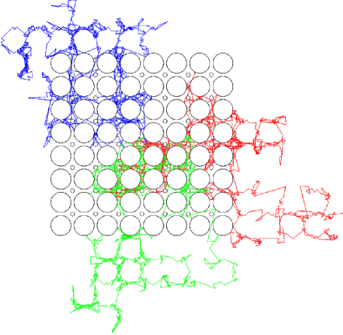
Billiard models constitute an important class of such models. Here, non-interacting point particles in free motion undergo elastic collisions with an array of fixed scatterers. Such models were introduced by Lorentz [Lor05], who modelled electron flow through an amorphous metal by point particles moving through a random array of hard spheres; such a model (with hard discs or spheres as the scatterers) is now termed a Lorentz gas. Several example trajectories of a periodic Lorentz gas are shown in Fig. 1.1.
Lorentz gases have been used to model neutron transport in dense media [CZ67] and can be viewed as modelling the flow of a dilute gas of light particles through a gas of heavy particles, in the limit where the ratio of masses of the light particles to those of the heavy particles goes to infinity [CC70]. The Lorentz gas is also a basic model in kinetic theory, since certain questions are simpler to answer in this context [vZvBD00, Hau74].
1.2.3 Hard-sphere fluids as billiard models
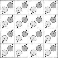
Furthermore, a hard-sphere fluid can be regarded as a billiard model in a high-dimensional phase space. The simplest example of this is a 2-disc periodic fluid consisting of two discs on a torus, or equivalently two discs in each copy of a periodically-repeated unit cell, as shown on the left of Fig. 1.2. Call the discs A and B, with radii and . Suppose we stand at the centre of disc A and look at the motion of disc B bouncing off disc A. We see the same dynamics as we would if a point particle located at the centre of B were colliding with a fixed disc of radius located at the centre of disc A. In this way the dynamics of the periodic fluid is equivalent to the dynamics of the periodic Lorentz gas model shown on the right of Fig. 1.2.

More generally, any hard-sphere fluid in a torus can be regarded as a billiard in a high-dimensional phase space, as follows. Consider hard spheres in a periodic box , with positions , velocities , masses and radii . The vector then specifies the instantaneous state of the system, where is the phase space of the dynamical system.
The total momentum is conserved, so we can change to a frame of reference in which the centre of mass is fixed at and the total momentum is , allowing us to restrict attention to a reduced phase space of lower dimension [Szá93]. Furthermore, regions of corresponding to configurations where the hard spheres overlap are not allowed; these excluded regions are high-dimensional cylinders in . The dynamics of the hard-sphere fluid then corresponds exactly to free motion in , together with elastic collisions on these cylinders, i.e. to billiard dynamics in the phase space [Szá93].
1.2.4 Transport in billiards
Billiards can be regarded as the simplest physical systems in which diffusion, understood as the large-scale transport of mass through the system, can occur: as pointed out in [Bun00], all that is required for diffusion to be possible is some mass which can move through the system, which is exactly the situation in billiards. Other transport processes have also been studied in billiards, e.g. electrical conduction [CELS93b, CELS93a], heat conduction [AACG99] and viscosity [BS96, Bun00, VG03].
In this thesis we consider only diffusion in periodic billiard models, where the scatterers form a periodic array. In this case the dynamics in the extended (unfolded) system can be obtained by looking at the dynamics on a single unit cell with perodic boundaries, i.e. a torus with scatterers removed, and keeping track of which lattice cell particles are in. The region exterior to the scatterers on the torus is then called the billiard domain. Since the particles are non-interacting, it is usual to set all velocities to by a geometrical rescaling, although in Sec. 4.7 we discuss the effect of a Gaussian velocity distribution.
1.3 Classical diffusion equation
Since we wish to describe dynamical systems as diffusive if their statistical behaviour looks like diffusion, we briefly review some features of the classical diffusion equation (also called the heat equation). This is a partial differential equation which models the empirically observed diffusion (flow / transport) of matter from regions of high concentration to regions of low concentration, and is one of the classical field equations of macroscopic physics. We begin by deriving the diffusion equation via a macroscopic balance equation.
1.3.1 Balance equations
Let be the density (per unit volume) of an extensive quantity. Then is a scalar time-dependent field depending on position in space and time , where is the number of spatial dimensions. Examples of such fields are the mass density of a substance, the heat content, the concentration of a chemical species, and the component of the momentum. We assume that is sufficiently smooth that we can differentiate with respect to space and time.
Consider a fixed region (a ‘volume’) in the space , with outward unit normal vector and boundary . The total amount of substance (or in general of the extensive quantity of which is the density) inside at time is ; this is the mass inside if is the mass density of a gas, for example.
This amount of inside can change over time by exactly two (local) mechanisms: can be created or destroyed inside , with source strength , the amount created per unit volume, per unit time; or can flow across the boundary of the volume , with flux vector per unit area, per unit time. This neglects non-local effects such as radiation.
Thus
| (1.1) |
Since is fixed, we can move the time derivative inside the integral. The divergence theorem then gives
| (1.2) |
for any fixed volume . This implies that444Taking all terms to one side gives an equation of the form . If is not (almost) everywhere , then it must be positive (without loss of generality) on some region of non-zero volume. Then , contradicting the assumption that the integral equal zero over any volume.
| (1.3) |
The equation (1.3) is termed a balance equation [KP98]. It forms the basis for deriving macroscopic evolution equations for any scalar field, and hence also vector and tensor fields by considering components. In order to derive such equations, we must specify and in terms of other known quantities using constitutive equations, which model the ‘constitution’ (behaviour) of a substance, to get a closed system of equations: see e.g. [KP98].
1.3.2 Derivation of the (anisotropic) diffusion equation
We now specialise to the case where is the concentration, or mass density, of a substance which is diffusing. If the mass of the substance is (locally) conserved, we have .555This is not the case, for example, if we have several reacting chemical species. The source of species A then contains terms describing the creation and destruction of A in the reactions (the total mass, however, being conserved). We then obtain a set of reaction–diffusion equations describing the spatio-temporal evolution of the concentration fields. Such equations can yield interesting spatial patterns [KP98]. We must now specify , a question which is considered at length in non-equilibrium thermodynamics [dGM84]. We consider only the (simplest) case, when Fick’s law is obeyed, so that the flux is a linear function of the concentration gradient, . (This can be viewed as a first-order approximation under the assumption of local thermodynamic equilibrium and slowly varying concentration profile [dGM84, KP98].) Hence
| (1.4) |
where is a second rank tensor called the diffusion tensor. The minus sign accounts for the empirical fact that matter diffuses from regions of high concentration to regions of low concentration. This is an example of a constitutive equation.
Assuming that is independent of position, we have
| (1.5) |
where are the components of the tensor with respect to a Cartesian coordinate system, and . We have defined the (symmetric) diffusion tensor as the symmetric part of , i.e. , with components . The antisymmetric part does not play any role, since the matrix of second partial derivatives of is symmetric. Substituting in (1.3) gives the (anisotropic) diffusion equation
| (1.6) |
We can also write this independently of coordinate system as
| (1.7) |
1.3.3 Solution of the diffusion equation in an unbounded domain
We consider the diffusion equation in one dimension, with independent of space:
| (1.8) |
We solve equation (1.8), a linear partial differential equation with constant coefficients, using a standard Green function method. For we define the Fourier transform of at time by
| (1.9) |
Fourier transforming (1.8) gives
| (1.10) |
an ordinary differential equation for , the solution of which is
| (1.11) |
Taking the inverse transform of this product gives a convolution:
| (1.12) | ||||
| (1.13) |
where is the initial concentration distribution and is the Green function (or propagator) for the diffusion equation on an unbounded -dimensional domain. This Green function is given by the Gaussian
| (1.14) |
with mean and variance
| (1.15) |
at time , and Fourier transform
| (1.16) |
We recall that the convolution operation is defined by
| (1.17) |
Multidimensional diffusion equation
In the multidimensional case, since is a symmetric tensor it is possible to choose an orthogonal coordinate system in which is represented by a diagonal matrix. In these new coordinates, the solution is a product of solutions of the 1D equation. Reverting to the original coordinates gives a multi-dimensional Gaussian [GS92] for a Dirac-delta initial condition.
1.3.4 Solutions of the diffusion equation as probability densities
Henceforth we regard the diffusion equation as describing the evolution of probability density functions representing probability distributions, as follows.
Let the initial condition at time be . Physically we are interested in non-negative with finite mass, i.e.
| (1.18) |
By normalising if necessary we can instead assume that
| (1.19) |
It then follows that and that the solution remains non-negative for all times , so that we can regard the diffusion equation as describing the time evolution of probability densities.
1.3.5 Calculation of moments from Fourier transform
We can calculate moments of a distribution directly from its Fourier transform as follows (see e.g. [RD77, Bal97]).
Differentiate (1.9) with respect to to get
| (1.20) |
and hence
| (1.21) |
Here we denote by the mean of the function with respect to the distribution at time . Similarly, higher moments can be obtained by differentiating repeatedly with respect to :
| (1.22) |
In a similar way, in the full multi-dimensional, anisotropic diffusion equation (1.6) for in dimensions, we use the multi-dimensional Fourier transform
| (1.23) |
where . Then we have, for example,
| (1.24) |
with higher moments calculated in an analogous way.
1.3.6 Asymptotic behaviour of moments of solutions of the diffusion equation
We assume that decays sufficiently fast at infinity for the relevant integrals to exist. Physically relevant sufficient conditions for this are, for example, that the initial condition has compact support, i.e. it vanishes outside a finite interval, or that the initial condition is exponentially localised, in the sense that
| (1.25) |
for some constant .
In this section we denote partial differentiation with respect to by a subscript , so that .
First moment
We first calculate the time dependence of the first moment (i.e. the centre of mass) of the solution of the diffusion equation. Differentiating (1.11) (the solution of the diffusion equation expressed in Fourier transforms) once with respect to , we have
| (1.26) |
so that using equation (1.21) twice, we obtain
| (1.27) |
Hence the mean position (centre of mass) is constant. So the second moment is the first non-trivial one.
Second moment
To simplify the calculation of the time evolution of the second moment, we now change to a coordinate system with the origin located at the centre of mass, i.e. we assume without loss of generality that .
Differentiating (1.11) again with respect to gives the second derivative
| (1.28) |
so that
| (1.29) |
(Note that .) Since was assumed to have compact support, is infinitely differentiable, by regularity results for Fourier transforms [Kat04]. Hence is a straight line with slope , which does not pass through the origin unless the initial condition is a Dirac delta (since the initial variance is only if the initial distribution is concentrated on a single point); the variance hence grows asymptotically linearly.
From the above result we can derive a relation between the diffusion coefficient and the rate of growth of the variance. Dividing (1.29) by and taking the limit gives
| (1.30) |
This result is known as the Einstein relation, since it was first obtained by Einstein [Ein85]. We also have
| (1.31) |
but note that the first limit can exist when the second one does not, for example if . Similarly in the multi-dimensional case we find
| (1.32) |
If the system has enough symmetry (Sec. 3.6), then we have for all , with all other components equal to , and
| (1.33) |
where is the spatial dimension and . We remark that this reduction of the diffusion tensor to a multiple of the identity tensor also occurs if the system is isotropic, i.e. has the same properties in any direction in space, but isotropy is a stronger condition than necessary for this reduction to happen.
1.3.7 Convergence of solutions of the diffusion equation to Gaussians
If the initial condition for the diffusion equation is at time , then the solution at time is given by the convolution
| (1.34) |
We are interested in the shape of the distribution for long times. In App. A we show that for suitable initial data the solution converges to a Gaussian when appropriately rescaled. This convergence requires the limiting function to be non-degenerate. Since tends to pointwise as , we must first rescale . We know from the above argument or from dimensional considerations that , where is a typical lengthscale and is a timescale. Hence we rescale by , putting
| (1.35) |
The first factor of is to normalise the integral of to .
In Chap. 4 we study the convergence to a limiting normal distribution of rescaled distribution functions in the context of billiards. For comparison, in App. A we consider the convergence of rescaled solutions of the diffusion equation to the limiting Gaussian. We show that converges pointwise to a Gaussian with variance :
| (1.36) |
where
| (1.37) |
is the Gaussian density with mean and variance . Furthermore the convergence is uniform with
| (1.38) |
for all and some constant which is independent of .
1.3.8 Numerical confirmation of decay
We numerically confirm the decay found in App. A by considering particular initial distributions. The first initial condition we consider is
| (1.39) |
where is the Dirac delta function at position . The diffusion equation with this initial condition is analytically soluble, with solution
| (1.40) |
so that the solution is smooth and rapidly decaying for any and hence fits into the class for which we can prove the convergence.
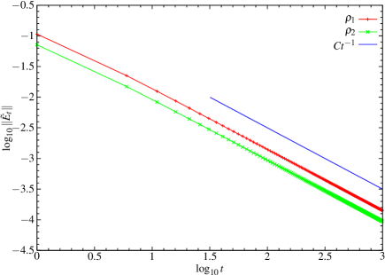
To verify the convergence numerically, we calculate , setting by rescaling time. Plotting the logarithm of this distance against the logarithm of time gives a straight line with slope , confirming the decay, as shown in Fig. 1.3.
1.3.9 Hallmarks of diffusion
We conclude from the above remarks that hallmarks of diffusion are the following features of the asymptotic behaviour as :
-
•
mean squared displacement growing asymptotically linearly in time , with constant of proportionality , where is the diffusion coefficient; and
-
•
convergence of the -rescaled position distribution to a non-degenerate Gaussian.
Here by ‘non-degenerate’ we mean that the limiting Gaussian has non-zero variance, or in higher dimensions that the covariance matrix is positive definite.
These are the statistical features which we will use to characterise a process as diffusive, together with a third dealing with convergence of rescaled paths to Brownian motion.
We remark that in general inhomogeneous physical systems, the rate of diffusion characterised by the diffusion coefficient can vary over the system. In such a case, we can say that we have diffusion if Fick’s law holds locally, i.e. if the flux of the diffusing quantity is locally proportional to its gradient [Cra75].
1.4 Statistical properties
Many dynamical systems, including important classes of billiards, are chaotic, in the sense that trajectories emanating from nearby initial conditions separate fast as time evolves. Any physical measurement has a limited precision, so that if we repeat an experiment several times then we cannot be sure that the initial condition is identical each time, but only that it lies within a certain tolerance. Averaging over the results of the experiments thus corresponds to averaging over a small ball of initial conditions as it spreads out over possible states of the system. This argument motivates the need for introducing probabilistic notions, namely ergodic and statistical properties, to study deterministic dynamical systems which are chaotic; see Chap. 2.
One of the main reasons for the interest in billiard models is the possibility of obtaining rigorous results on their ergodic and statistical properties: see e.g. [BS81, BSC91]. The techniques are most highly developed for dispersing billiards such as the Lorentz gas, where the curved, convex scatterers cause nearby trajectories to separate exponentially fast. In fact, Lyapunov exponents (which measure the rate of separation) exist and are non-zero almost everywhere for the billiard map, so that the system is hyperbolic (chaotic). Due to the Hamiltonian nature of the system, the Lyapunov exponents come in positive–negative pairs, so that at least one Lyapunov exponent is positive almost everywhere [CM01, Gas98]; further, the Kolmogorov–Sinai entropy, which measures the rate of generation of information in time, is positive [Gas98]. These are standard indicators of the chaotic nature of the system [ER85].
Hard-sphere fluids are only semi-dispersive, due to the flat, neutral directions along the cylinder axis in the many-particle phase space; this makes their rigorous analysis much harder: see e.g. [Bál99] for a review. Nonetheless, a rigorous proof of the celebrated Boltzmann ergodic hypothesis has recently been achieved for hard discs () and spheres (): see references in Sec. 2.5.4.
The main focus of this thesis is deterministic diffusion, a statistical property of certain dynamical systems, including certain classes of billiards. A definition often used in the physical literature is that a system is diffusive if the mean squared displacement grows proportionally to time , asymptotically as . However, there are stronger properties which are also characteristic of diffusion, which a given system may or may not possess: (i) a central limit theorem may be satisfied, i.e. rescaled distributions converge to a normal distribution as ; and (ii) the rescaled dynamics may ‘look like’ Brownian motion. See Chap. 2 for details.
Recently there has been much interest in the question of which microscopic features are necessary for a system to exhibit strong ergodic and statistical properties. The proofs of these properties for dispersive billiards depend crucially on the fact that they are hyperbolic, but numerical evidence has been given that systems with weaker chaotic properties may also show strong statistical properties, for example the polygonal billiard channels studied in Chap. 5.
1.5 Overview of thesis
Chapter 2 reviews concepts from dynamical systems, probability theory and ergodic theory which we require to discuss deterministic diffusion. Chapters 3–6 present our results on deterministic diffusion in three types of billiard model: a 2D periodic Lorentz gas with a two-dimensional parameter space (Chaps. 3 and 4); several classes of polygonal billiard channel (Chap. 5); and 3D periodic Lorentz gases (Chap. 6). Conclusions are presented in Chap. 7, followed by several appendices giving technical details of results needed in the main text; we expect that many of these results are already known, but in several cases we were unable to find suitable references.
The discussion in each chapter can be thought of in terms of three related threads. The first is mathematical: to what extent do rigorous results hold beyond their immediate range of applicability, and can we understand more precisely the statistical behaviour described by those results? The second is physical: how do geometrical features affect the dynamics and statistical properties of the system? The third is statistical: how can we best estimate statistical properties from numerical data?
Chapter 2 Statistical properties of dynamical systems
In this chapter we review in what sense deterministic dynamical systems ‘look like’ stochastic processes. We make a (somewhat arbitrary) distinction between ergodic properties and statistical properties: the former deal with general theorems referring to large classes of observables, whereas the latter hold only for observables with a certain degree of smoothness, are related to rates of convergence in ergodic theorems, and are of physical relevance.
2.1 Dynamical systems and stochastic processes
2.1.1 Invariant measures
Let be the flow of a continuous () or discrete () dynamical system with phase space . Measures are defined on some -algebra on . Our dynamical systems will be defined on metric spaces, so that we can take, for example, to be the Borel measurable subsets of . Then any physically relevant subset of will be in , and from now on we will usually refer to subsets of without explicitly mentioning .
Suppose that we start the evolution of the dynamical system with a distribution of initial conditions described by the measure . This distribution will evolve in time to the measure given by
| (2.1) |
here the right hand side defines the meaning of the push-forward .
A particularly simple and interesting case occurs if the measure is preserved by the system, or is invariant, as follows. We say that is invariant with respect to the flow if, for all , , or equivalently if
| (2.2) |
Here we also require that be measurable with respect to , i.e. such that for all . In the discrete time case, where the dynamics is given by a map , it is enough to have for all measurable sets .
Natural invariant measures
Some systems possess natural invariant measures if the dynamics preserves some structure. The main class of interest to us is Hamiltonian systems, which preserve Liouville measure: see Sec. 2.5 in the case of billiards and [KH95, Chap. 5] for other examples. We are then most interested in statistical properties with respect to these measures.
2.1.2 Dynamical systems with invariant measures as stationary stochastic processes
Fix an observable (that is, a quantity that we could in principle measure when the system is in different states in phase space) and look at . Given a measure on , we can regard as a collection of random variables indexed by time, so that we have a stochastic process [GS92].
If the measure is invariant, then the process is stationary, which means that for all , all and all , the families
| (2.3) |
have the same joint distribution as each other [GS92]. The proof is as follows. For two times and and two sets , we have
| (2.4) | ||||
| which by the measure-preserving property of is equal to | ||||
| (2.5) | ||||
An analogous argument holds for times and sets; hence the random variables form a stationary stochastic process.
2.2 Ergodic properties
Ergodic properties with respect to an invariant measure can be thought of loosely as a measure-theoretic description of chaoticity. There is a hierarchy of increasingly strong properties; the ideas originated in statistical mechanics: see e.g. [Dor99]. A general reference is, for example, [CFS82].
2.2.1 Ergodicity
In the billiard systems we study there is a natural invariant measure , namely Liouville measure (see Sec. 2.5), which we regard as fixed in the following.
Suppose that the invariant measure is finite, i.e. . Then we can normalise to get a probability measure with . The flow is ergodic with respect to if111We continue to suppress the necessity of having . for all , we have
| (2.6) |
i.e. any set which is invariant under the flow has measure , so that it is trivial from the point of view of measure theory, or has measure , so that it covers the whole space except for a set of measure .
2.2.2 Birkhoff ergodic theorem
Let be an invariant probability measure for the dynamical system , and let be integrable. Then Birkhoff’s ergodic theorem states (see e.g. [CFS82]) that the limit
| (2.7) |
exists for almost all with respect to the measure , and we call the time average of . Furthermore, if also the system is ergodic, then
| (2.8) |
so that time averages are almost everywhere (a.e.) equal to the space average with respect to the ergodic invariant measure .
The motivation for this theorem came originally from Boltzmann, who had the idea that a sufficiently complicated dynamical system should explore the whole accessible phase space, an idea known as the ergodic hypothesis. This has recently been proved for hard-sphere fluids in a series of papers [Sim, Sim04, Sim03, SS99].
2.2.3 Mixing
The flow is mixing with respect to the invariant measure if for any sets , we have
| (2.9) |
Mixing implies ergodicity. An important interpretation for us is that mixing is equivalent to weak convergence of densities: see App. C.
There is also a notion of weak-mixing, intermediate in strength between ergodicity and mixing. For discrete time systems we say that a transformation preserving a measure is weak-mixing if for any , we have
| (2.10) |
For comparison, there is a characterisation of ergodicity in similar terms, stating that is ergodic if for any we have
| (2.11) |
See [Wal82, CFS82] for detailed comparisons of the different notions, and [CFS82] for formulations for continuous-time systems.
2.2.4 K-systems
K-systems have very strong ergodic properties: in particular their Kolmogorov–Sinai entropy is positive. See e.g. [Sin94, p. 71] for the definition. K-systems are multiply mixing (a generalisation of mixing), mixing and ergodic.
2.3 Statistical properties: probabilistic limit theorems
We now turn to statistical properties, reviewing the application of results from the theory of stationary stochastic processes to the context of dynamical systems.
Diffusion in billiards concerns the statistical behaviour of the particle positions. Denoting the position at time by and restricting attention to the first component , we can write
| (2.12) |
where , the first velocity component. This expresses solely in terms of functions defined on the torus, so that in a sense we have reduced a spatially extended problem (spreading out over an infinite lattice) to a problem on the torus. Equation (2.12) shows that the displacement is in some sense a more natural observable than the position in this context.
In the above we are regarding as the observable
| (2.13) |
which returns the first component of the velocity of the initial condition, so that is the first velocity component at time starting from the initial condition .
More generally, we can consider integrals of the form in (2.12) over other observables ; these are important in the study of other transport processes, for example [Bun00]. The question we wish to answer then concerns the distribution of accumulation functions of the form [CY00]
| (2.14) |
in particular in the limit as .
The integral in (2.14) is a continuous-time version of a Birkhoff sum
| (2.15) |
where the are stationary random variables. We are thus interested in statistical properties, for example means and shapes of limiting distributions, of sums and integrals of stationary random variables.
Intuitively, if the correlations between the decay sufficiently fast, then they are asymptotically independent, and we can hope that the classical limit theorems for independent and identically distributed random variables can be extended to the stationary case. The Bernstein method, summarised below, is a rigorous justification for this.
2.3.1 Averages
The simplest statistical properties to study are averages of observables. If is an observable on the phase space of the dynamical system, then we denote the mean of the observable by
| (2.16) |
Here, is the distribution of initial conditions and denotes the expectation of the random variable with respect to the probability measure .
We will be interested in the evolution over time of such averages when the observable involves the flow . A key role is played by the mean squared displacement at time , denoted
| (2.17) |
In the final expression in (2.17), the dot denotes the variable over which the average is taken. We will usually think of this mean squared displacement as a function of time , so that it is convenient to use the notation , which makes this dependence explicit.
The physical interpretation of the above definition is as an average over initial conditions of the time-dependent observable. An alternative point of view is to regard as an average over the evolved probability distribution at time starting from a distribution at time ; the average is then over a fixed observable at points determined by evolving the initial conditions in time.
2.3.2 Central limit theorem: independent, identically distributed case
Let be independent and identically distributed (i.i.d.) random variables with mean and variance . We are interested in statistical properties of the accumulation function
| (2.18) |
as . We have
| (2.19) |
so that if we normalise by , setting , then we get
| (2.20) |
Since the variances of the are now independent of , we may hope that the distributions converge in shape to some limiting distribution.
With the above conditions, the classical central limit theorem (see e.g. [Fel71, Dur96]) states that
| (2.21) |
so that the rescaled accumulation functions converge in distribution to a normal distribution.
We recall the definition of this notion of convergence [GS92, Bil68]. Let be a sequence of real-valued random variables with distribution functions , so that . We say that the sequence converges in distribution to the random variable , with distribution function , written , if at all where is continuous. There is a generalisation of this concept which applies in much more general situations: see App. D.
2.3.3 Central limit theorem: stationary case
If now the are no longer independent but they are stationary, we have
| (2.22) |
where the autocorrelation function of is
| (2.23) |
and both denote averages (expectations) over the invariant measure. It follows that
| (2.24) |
provided exists. A sufficient condition for this222Note that is not sufficient, since is divergent for . On the other hand, is not necessary either, since e.g. for the sum is convergent for [Rud76]. is that for some .
Now we may again hope/expect that
| (2.25) |
We can also regard the central limit theorem as describing the distribution of ‘fluctuations’ around the mean in the Birkhoff ergodic theorem. (Note that the Birkhoff ergodic theorem is a version of the strong law of large numbers for stationary processes [Dur96].)
2.3.4 Central limit theorem for stationary processes: Bernstein method
The Bernstein method can be used to prove results of central limit theorem (CLT) type for stationary processes, based on the idea that if decays sufficiently fast then the are asymptotically independent and we can reduce to the case of independent random variables.
The method works as follows (see e.g. [Dur96, Chap. 7] and [Bil68]). Split the sum up into alternate blocks of length and of length , so that , , , etc.; see Fig. 2.1.

If is sufficiently large then the are almost independent; on the other hand, if is small compared to then the sum of the small blocks is small compared to the total size of the sum . In a suitable limit we can thus reduce to the independent case, with an error which tends to .
2.3.5 Rate of mixing
For the above to work, we need to show for a given stationary sequence that the correlations decay fast enough, i.e. that we have a fast enough rate of mixing. There are various sufficient ‘mixing conditions’ for the central limit theorem to hold: see e.g. [Dur96, Bil68, Dav94] in the context of probability theory, and [Den89, Liv96] in the specific context of dynamical systems.
2.3.6 Functional central limit theorem
The central limit theorem quoted above deals with one-dimensional distributions. There is a multi-dimensional version, where multi-dimensional distributions converge to multi-dimensional normal distributions. If also a further technical condition, called tightness, is satisfied, then the probability distribution on the space of continuous paths which is induced by the dynamical system converges weakly to a continuous-time stochastic process. If further the correlations behave correctly, then the limit will be the particular case of Brownian motion. Such a result is known as a functional central limit theorem (i.e. a version of the central limit theorem for paths represented by functions). This is also called the weak invariance principle.
2.3.7 Almost-sure invariance principle
The strongest type of statistical property is known as an almost-sure invariance principle, since it says that a stochastic process can be written, almost surely, as the sum of a Brownian motion on a suitable space, together with an error which can be bounded in a precise way: see e.g. [PS75, DP84, MT04].
2.3.8 Transition from discrete-time to continuous-time
In billiards, we are interested in statistical properties of the physical continuous-time dynamics. Currently these are not directly available, due to the lack of information on decay of correlations in continuous time; rather they are derived from the results on the billiard map, using the fact that the flow is a suspension flow over that map.
We refer to App. B for the definition of suspension flows and for a statement of the key theorem relating the central limit theorem for the flow to that of the map. We give here a derivation of the Green–Kubo formula from the Einstein formula for the diffusion coefficient in continuous time, valid only if the velocity autocorrelation function decays sufficiently fast, which for billiards has not yet been proved [CY00]. References containing similar derivations include [vB82, Det00, BY91, RD77]. We remark that recent results333 [Stretched exponential bounds on correlations for Hölder-continuous observables for the 2D periodic Lorentz gas were recently proved in [Che07].] have shown the exponential decay of correlations in continuous time for Hölder observables of Anosov geodesic flows [Dol98, Che98] and contact flows [Liv].
We take as a starting point the Einstein formula
| (2.26) |
Using , we have
| (2.27) |
Here we have used the fact that the averages are invariant with respect to time translation, due to the stationarity of the stochastic process; we also performed a change of variables from to .
We now change the order of integration, obtaining
| (2.28) |
Hence
| (2.29) |
We can now define a finite-time diffusion coefficient , an estimate for the (infinite-time) diffusion coefficient based on the information available up to time . There are two possible ways to do this. Using the Einstein definition, we have
| (2.30) |
where is the velocity autocorrelation function. Hence the diffusion coefficient
| (2.31) |
exists if: (i) , i.e. is integrable; and (ii) as . In fact (ii) follows from (i) by integrating by parts, so that a necessary and sufficient condition for the existence of the diffusion coefficient is that is integrable.
The equation (2.31), relating the time integral of the velocity autocorrelation function to the transport coefficient , is a Green–Kubo relation [Dor99]; Green–Kubo formulae can be found for all transport coefficients [EM90, Gas98], e.g. via linear response theory [EM90], expressing the transport coefficient as a time integral of the autocorrelation function of the flux of the quantity being transported.
Another possible definition of a finite-time diffusion coefficient , which is more closely related to the numerical method we shall use later [Bal97, AT87], is to define using the local slope of the mean squared displacement :
| (2.32) |
From (2.29), we have
| (2.33) |
so that the fundamental theorem of calculus gives
| (2.34) |
This definition avoids the slowly-decaying tail of the first definition [Bal97]. Further, if we have a bound on the rate of decay of correlations then we can use (2.34) to estimate the error resulting from using the finite-time diffusion coefficient instead of its infinite-time limit . For example, if correlations decay exponentially as
| (2.35) |
then we can estimate
| (2.36) |
Hence this difference tends very rapidly to zero, as seen in numerical simulations. However, obtaining the constants and , even numerically, is difficult or impossible.
If, on the other hand, correlations decay only algebraically as
| (2.37) |
then
| (2.38) |
This error tends to zero very slowly for small , so that the finite-time estimation method for any practical time has an additional uncertainty built in.
2.4 Definition of deterministic diffusion
There is no single definition of deterministic diffusion; instead, we say that a dynamical system is diffusive if one or more of the following hierarchy of statistical properties holds. The idea is that the statistical properties behave to some extent like those of solutions of the diffusion equation described in Sec. 1.3, or those of Brownian motion (see below). We use terminology suitable for diffusion in billiards, although these properties are also relevant for more abstract dynamical systems.
-
(a)
the mean squared displacement grows linearly asymptotically;
-
(b)
the position or displacement distribution, rescaled by , converges in distribution to a non-degenerate Gaussian, i.e. a central limit theorem holds; and
-
(c)
the whole process, suitably rescaled, converges in distribution to a Wiener process.
Properties (a) and (b) are based on the corresponding properties of the diffusion equation, although property (b) will in general only hold at the level of weak convergence, whereas in the classical diffusion equation there is pointwise (and even uniform) convergence of the densities. Property (c) says that the process, when suitably rescaled, looks like Brownian motion, which can be thought of as a probabilistic model of diffusion. We have the implications444 [In fact, as was pointed out to me by Ian Melbourne, (b) does not imply (a) in general. However, in billiards, they tend to go together – to know which scaling factor to use in the central limit theorem, it is necessary to calculate the mean squared displacement.] (c) (b) (a), so that (c) is the strongest property. We now give precise versions of these statements.
(a) Asymptotic linearity of mean squared displacement
The limit
| (2.39) |
exists, so that the mean squared displacement (the variance of the displacement distribution) grows asymptotically linearly in time:
| (2.40) |
where is the diffusion coefficient. In dimensions, letting be the th component of the displacement, we have
| (2.41) |
where the are components of a symmetric diffusion tensor.
(b) Central limit theorem: convergence to normal distribution
Scale the displacement distribution by , so that the variance of the rescaled distribution is bounded. Then this distribution converges weakly, or in distribution, to a normally distributed random variable [GN90, CY00]:
| (2.42) |
In the -dimensional case, this means that
| (2.43) |
where denotes the probability of the event inside the parentheses with respect to the initial distribution of the random variable , and is the variance of the limiting normal distribution. In dimensions, this is replaced by similar statements about probabilities of -dimensional sets. This is the central limit theorem for the random variable . From (a) we know that in 1D, the variance of the limiting normal distribution is ; in dimensions, the covariance matrix of is given by the matrix [BS81, DC00].
(c) Functional central limit theorem: convergence of path distribution to Brownian motion
Consider the following rescaling of the whole path of the process:
| (2.44) |
where . The scale is the ‘natural’ scale coming from (b). This rescaling ‘squashes’ the entire path of the process onto the interval , so that we can compare paths at different times. In fact, we compare the induced probability measures on the space of continuous functions .
We say that the process satisfies a functional central limit theorem if the probability distribution of the rescaled paths of the process converges weakly to Wiener measure (Brownian motion) with covariance matrix as in (b), as :
| (2.45) |
This is known as a functional central limit theorem, or weak invariance principle [CY00].
This makes precise the sense in which looks like Brownian motion on long length and time scales. In the following sections we discuss in more detail the meaning of the above statement, by showing how diffusion can be regarded as a stochastic process and in what sense these rescaled processes converge to diffusion processes.
2.4.1 Diffusion as a stochastic process
As recalled in Sec. 1.3, diffusion is described classically by the diffusion equation
| (2.46) |
We would like a microscopic model which gives behaviour on a macroscopic level consistent with this equation. Following Einstein and Wiener (see e.g. [Gar85]), we look for a stochastic process , determined by the probability density of a particle being at position at time given that it started at at time . Based on physical reasoning, we impose that the sample paths of the process should be continuous, and that displacements should be independent of the history of the particle motion up to time .
Under certain technical conditions, then satisfies the equation
| (2.47) |
which is known as Kolmogorov’s forward equation or the Fokker–Planck equation [Gar85]. The drift vector and the diffusion tensor give the mean and variance, respectively, of infinitesimal displacements at position and time [Gar85].
If the system is homogeneous, then and are independent of and . If the system is also sufficiently symmetric, then the drift is zero and the diffusion tensor is a multiple of the identity tensor. The stochastic process is then Brownian motion, and the Fokker–Planck equation (2.47) reduces to the diffusion equation (2.46). (We remark that the factor in (2.47) occurs naturally in the probabilistic setting, and often leads to a discrepancy between the probability and physics literature.) A general diffusion process, however, can be inhomogeneous in both space and time.
Brownian motion is defined as follows [Dur96]. A standard one-dimensional Brownian motion (also called the Wiener process) is a real-valued stochastic process , , such that:
-
(i)
For all , if , then the increments are independent random variables.
-
(ii)
If , then is a normal random variable with mean and variance , so that
(2.48) -
(iii)
With probability , the function is continuous.
Standard -dimensional Brownian motion is then the vector process , where each is an independent standard 1D Brownian motion.
Another approach to study such diffusion processes is via stochastic differential equations (SDEs) [Gar85]. The above process corresponds to solutions of the SDE
| (2.49) |
where is an -dimensional Brownian motion and . This form makes more explicit the infinitesimal increments referred to above, and is now in a form which is more suitable for numerical simulation.
2.4.2 Weak convergence to Brownian motion
We must make precise what we mean by saying that
| (2.50) |
The rigorous definition of this notion of weak convergence is given in App. D; see [Bil68]. Necessary and sufficient conditions are [Bil68] (1) that the finite-dimensional distributions of the process converge to those of Brownian motion; and (2) that the class of induced measures on path space is tight: see App. D for the definition.
Property (1) means that for any , any times , and any reasonable sets in , we have
| (2.51) |
This is called the multi-dimensional central limit theorem in [Che95]. The right-hand side can be expressed as a multi-dimensional integral over Gaussians, as follows. We see that555The probability that exactly is , but the argument can be made rigorous.
| (2.52) | ||||
| (2.53) | ||||
| (2.54) |
since by the definition of Brownian motion , the events and are independent, and is normal with mean and variance ; here is the Gaussian probability density function with that mean and variance. Integrating over all and , we have
| (2.55) |
with a similar expression for the right hand side of (2.51).
Since if and only if , the multidimensional central limit theorem becomes
| (2.56) |
setting and then renaming the times as . This relation was used in [DC00] as the definition of a diffusive process, although the functional central limit theorem is a stronger statement which also requires tightness. We remark that another name for the functional central limit theorem is the weak (or Donsker) invariance principle [CY00].
In general, we may have convergence to a more general diffusion process than Brownian motion. For example, in [DGL81] it was shown that the motion of a large particle embedded in an infinite ideal gas converges to an Ornstein–Uhlenbeck process. In the case of the periodic Lorentz gas, however, we have time-independent dynamics defined on a system which is space-homogeneous and symmetric on a large scale; the only possible limiting diffusion process which satisfies these conditions is Brownian motion.
2.4.3 Further remarks
An important part of the above limit theorems is proving that the limiting distribution is non-degenerate, i.e. that the diffusion tensor is positive definite [Bun00]. In general, we can consider the above limit theorems for an arbitrary observable .
We will mostly consider -dimensional projections (marginals) of the above distributions; we can equivalently regard this as studying the limit theorems for being one component of , which follow from the multi-dimensional results stated above.
2.4.4 Discussion of definitions
Property (c) makes precise in what sense a dynamical system looks like Brownian motion when correctly rescaled. This is the strongest, and so in some sense the best, property with which we could define deterministic diffusion (i.e. a dynamical system is diffusive when it satisfies property (c)). However, there are very few physically relevant systems which have been proved to satisfy (c). Interest in the periodic Lorentz gas comes in large part from the fact that it is one of the only such systems; another is the triple linkage [HM03]. As mentioned above, in general we may instead have convergence to some other diffusion process.
The multi-dimensional central limit theorem part of (c) was studied in [DC00], where both Lorentz gases and wind–tree models were found to obey it, tested for certain sets and certain values of . However, as stated in [DC00], (c) is difficult to investigate numerically, and the results in that paper seem to be the best that we can expect.
Property (b), the central limit theorem, has been shown for large classes of observables in many dynamical systems (see e.g. [Che95] and references therein), but again they are not often physically relevant systems. Property (b) was used in [GN90] as the definition of a diffusive system, but does not seem to have been applied in the physics literature; this is the approach taken in Chap. 4.
Most emphasis in the physical literature is placed on property (a): many authors define a system to be diffusive if only property (a) is verified (numerically), e.g. [KD00, ARdV02, DC01]. Many types of system are diffusive in this sense, including 1D maps [KD99], Lorentz gases (periodic and random) [BS81, KD00, DC01] and Ehrenfest wind–tree models, both periodic [ARdV02] and random [DC01].
The implication (c) (b) always holds, and (a) and (b) usually go together. The reverse implications (a) (b) and (b) (c) hold only under certain additional conditions: see e.g. [Che95]. It is thus of interest to ask if dynamical systems showing property (a) also show properties (b) and (c). For example, in [KC89] a disordered lattice-gas wind–tree model was reported as having an asymptotically linear mean squared displacement, but a non-Gaussian distribution function, i.e. (a) but not (b). However, disorder can lead to trapping effects which cannot occur in periodic systems [ARdV02]; we are not aware of a periodic (and hence ordered) billiard model with a unit-speed velocity distribution which shows (a) but not (b), although in Sec. 4.7 we show that this can occur with a Maxwellian velocity distribution.
2.4.5 Approach via cumulants
Several papers have approached property (b) by studying higher order cumulants of the distribution, e.g. [ARdV02, DC01]. A normal distribution has all cumulants higher than the second equal to zero. It thus seems that we need all cumulants of the rescaled displacement distribution to tend to zero as for the distribution to approach a normal distribution; this was stated in [DC01, p. 790], for example.
In fact, the weak type of convergence occurring in the central limit theorem (convergence in distribution) does not in general require higher moments and cumulants even to exist: a faster rate of decay of correlations is necessary to ensure the existence of higher cumulants than is required for the central limit theorem to hold: see [vB82, CD00].
Higher cumulants are instead related to large deviations, describing behaviour in the tails of the distribution [Gas98, Sec. 7.3.6]. We show in Chap. 5 that a class of polygonal billiard channels which was found in [ARdV02] to have rapidly-growing cumulants nonetheless appears to satisfy the central limit theorem.
2.5 Rigorous results on billiards
In general, a billiard table is a Riemannian manifold with a piecewise smooth boundary. The dynamics is given by geodesic flow away from the boundary and specular reflection (elastic collision) at the boundary. Here we restrict attention to two-dimensional periodic Lorentz gases, where non-interacting point particles in free motion on a torus-shaped billiard table undergo elastic collisions with a set of fixed scatterers. We give only enough detail for our purposes, and refer to [Tab95], [CFS82, Chap. 6] and [CM01, Chap. 4] for further information666 [An excellent recent reference on chaotic billiards is [CM06].] .
2.5.1 Continuous-time dynamics
We denote by the billiard domain, i.e. the available region where particles can move, given by
| (2.57) |
where the scatterers are non-intersecting discs in the case of the periodic Lorentz gas. We visualise the torus as a square with periodic boundary conditions, as in Fig. 2.2.

Each particle moves in a straight line within at constant velocity until it hits the boundary at a point on the boundary of scatterer . It then undergoes an elastic collision, giving a new velocity
| (2.58) |
after collision, where is the outward normal vector at to the scatterer . The particle continues its motion by alternation of straight line motion and elastic collisions with the boundary.
The above prescription defines a continuous-time dynamical system given by a flow
| (2.59) | |||
| (2.60) |
where is the tangent bundle to , i.e. the set
| (2.61) |
where is the tangent space to at the point .
Since the speed is preserved, it is customary to take all particles with unit speed777We consider non-constant speed distributions in Sec. 4.7.. We can thus restrict attention to the new phase space given by the unit tangent bundle888The identification of the unit tangent bundle with the direct product is not in general valid, but it does hold for the simple situation we consider.
| (2.62) |
where
| (2.63) |
and the flow , which we call the billiard flow. We can parametrise the space with coordinates , where are position coordinates and is the angle of the velocity vector.
We remark that for billiard tables with corners, where two smooth parts of the boundary touch at a non-zero angle, the trajectory cannot be continued if it exactly hits a corner. However, the set of all such trajectories has measure .
2.5.2 Billiard map: Poincaré section
As is often the case in dynamical systems, it turns out to be technically easier to study a Poincaré section of the flow. A natural cross-section is given by
| (2.64) |
i.e. the set of vectors whose base points lie on a scatterer and which point into the interior of the billiard domain. This cross-section forms a two-dimensional surface in the three-dimensional phase space . One way of parametrising is to take as coordinates the arc length around the scatterer of the point of collision (from some reference point), and the angle between the velocity vector and the normal vector [CM01]. Alternatively we can take the arc length around the scatterer and the sine of , giving canonically conjugate Birkhoff coordinates [Gas98, Chap. 5]. In general we must also keep track of a label denoting which scatterer was hit. The flow then induces an invertible map which maps one collision into the next, called the billiard map.
The billiard flow can now be regarded as a suspension flow over , under the free path length function , where is the length of the collision-free part of the trajectory emanating from the initial condition . Suspension flows are treated in detail in App. B.
2.5.3 Measures
Since the billiard flow is Hamiltonian, it preserves a natural invariant measure , called Liouville measure, given by999This is a useful shorthand for the statement (2.65)
| (2.66) |
where etc. denote Lebesgue measure in the respective coordinate, and is a normalising constant chosen so that . This measure induces a measure on which is invariant under , given by [CM01]
| (2.67) |
For a 2D billiard (i.e. one for which the dynamics is restricted to a plane), we have
| (2.68) |
and
| (2.69) |
2.5.4 Ergodic and statistical properties
The ergodic and statistical properties of billiards have been the object of intense scrutiny since the seminal work of Sinai [Sin70], where the K-property of the periodic 2-disc fluid was proved. All of the proofs depend on the hyperbolicity of scattering billiards, i.e. the existence of stable and unstable directions; for details see [CM06, CM01, Gas98, Tab95] and the references cited below. A few of the key rigorous results for dispersing and semi-dispersing billiards are:
2.6 Numerical evaluation of statistical quantities
To evaluate numerically statistical quantities such as the mean squared displacement, we use a simple Monte Carlo method. We take a large sample of size of initial conditions chosen uniformly with respect to Liouville measure in one unit cell using a random number generator: the positions are uniform with respect to Lebesgue measure in the billiard domain , and the velocities are uniform in the unit circle , i.e. with angles between and , and unit speeds. These evolve after time to ; the distribution of this ensemble then gives an approximation to that of .
We use the Mersenne Twister random number generator [MN98], which seems to be considered to be one of the best-performing generators; we have also done some comparisons with a standard rand implementation. Since our random numbers determine only the initial conditions, and since the system is strongly mixing, we do not expect the choice of random number generator to be important, provided the initial conditions are sufficiently well distributed through the phase space, so that no small regions with important dynamical effects are omitted.
We denote averages over the initial conditions, or equivalently expectations with respect to the distribution of , by . Approximations of such averages can now be evaluated via [PTVF92]
| (2.70) |
The infinite sample size limit, although unobtainable in practice, reflects the expectation that larger will give a better approximation.
Lyapunov instability
The Lyapunov instability in dispersing billiards implies that numerical simulations of trajectories will not be accurate beyond a time where the uncertainty in the initial condition has grown exponentially to , so that some authors do not allow any data obtained beyond that time [GG94]. However, most physics papers implicitly reject this argument by presenting long-time results from simulations, and we shall also do this, whilst being careful about other sources of error in statistical calculations. One partial justification for this comes from shadowing [CM06]: in certain hyperbolic systems, it can be proved that there is a true trajectory close to a simulated trajectory. The difficulty in billiards comes from the discontinuous nature of the dynamics; nonetheless, some results of shadowing type were proved in [KT92]. We are not aware of any papers which investigate shadowing in particular billiard models, but early numerical investigations of the validity of numerical estimates of ergodic properties for uniformly hyperbolic systems can be found in [BCG+78, BCG+79].
Chapter 3 Geometry-dependence of the diffusion coefficient in a 2D periodic Lorentz gas model
3.1 Two-dimensional periodic Lorentz gas model
A periodic Lorentz gas is a periodic billiard with disjoint circular scatterers (discs). The term is also applied to other periodic billiards of dispersing type with scatterers of more general shape: see e.g. [HKG02].
In this chapter and the following one we study aspects of deterministic diffusion in a particular 2D periodic Lorentz gas model introduced below: here we consider only the mean squared displacement and the diffusion coefficient, while in Chap. 4 we examine the shape of distributions.
3.1.1 Finite horizon condition
Periodic Lorentz gases were shown in [BS81, BSC91] to be diffusive (Sec. 2.4), provided they satisfy the finite horizon condition: there is an upper bound on the free path length between collisions. If this is not the case, so that a particle can travel infinitely far without colliding with any scatterers (the billiard has an infinite horizon), then corridors exist, which allow for fast-propagating orbits. This leads to super-diffusive behaviour, in the sense that the mean squared displacement grows like (which is faster than ), as has recently been proved in [SV07], after heuristic and numerical arguments [FM84, ZGNR86] and analytical evidence [Ble92] were previously given. There is a more detailed discussion of statistical behaviour in the infinite-horizon regime in Sec. 6.4.
We are mainly interested in normal diffusion, so that we wish to restrict attention to values of the geometrical parameters for which there is a finite horizon. The simplest periodic two-dimensional lattice111We consistently use the term ‘lattice’ in the sense of physics to mean any periodic structure. Mathematicians instead use the term in the narrower sense of the set of points in of the form , where the are basis vectors of and ; these are called Bravais lattices in physics [AM76]. is the square lattice. To allow the possibility of diffusion in a square lattice, the scatterers must not touch or overlap: if they do, we obtain a localised regime where any particle is trapped in a bounded region of space, so that the diffusion coefficient is necessarily . However, non-touching scatterers in a square lattice always imply an infinite horizon: trajectories parallel to the lattice axes and passing sufficiently close to the centre of a unit cell never collide.
For this reason a periodic Lorentz gas on a triangular lattice is often used, where there is a finite horizon when the non-touching discs are sufficiently close together: see e.g. [MZ83, KD00]. We instead elect to retain a square lattice model, blocking all possible corridors by adding an additional disc at the centre of each cell.
3.1.2 Model studied
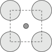
The model which we focus on, previously studied in [GG94, Gar97], consists of two inter-penetrating square lattices of discs; they have the same lattice spacing , and radii and , respectively, and are arranged such that each unit cell of the -lattice contains a -disc at its center. Part of the infinite system is shown in Fig. 3.1 and the geometrical parameters are defined in Fig. 3.1.


We were led to this model as a cross-section of the 3D model presented in Chap. 6, independently of [GG94, Gar97], although as described above, it is a natural model to consider. The same model has also been studied in [BDLR02, BDL00] in a different context. The two-dimensional parameter space of this model allows us to vary independently, and hence study the effect of, two physical quantities: the size of exits of each unit cell, and the accessible area of a unit cell. This is not possible in the standard triangular Lorentz gas.
3.1.3 Length scale
Since the speed is conserved, scaling the geometry by a constant factor does not alter the essentials of the dynamics, just the time-scale on which it occurs. We may hence use dimensionless units such that the speed is equal to and we are free to choose a length scale.
In this thesis we use one of two choices of length scale: in analytical calculations it is often convenient to fix and vary and ; while in numerical calculations we often fix and vary and . Where necessary we distinguish the latter case using tildes, writing
| (3.1) |
3.1.4 Parameter space
Garrido [Gar97] derived the ‘phase diagram’ of the model, showing the regions in parameter space corresponding to the various localised, finite horizon and infinite-horizon regimes. Here we correct this diagram by including the following features that were incorrectly treated in [Gar97]: (i) the system is symmetrical under interchange of and ; and (ii) the finite-horizon regime is smaller than was found in [Gar97]. We fix but omit the tildes on and . The derivation, which reduces to geometrical considerations, is useful since it provides pointers for the geometrically more involved calculation for the 3D model in Chap. 6.
If we interchange the radii and , then the resulting structure is the same as the initial one, except for a translation by the vector . Hence the statistical properties are the same, so that the whole phase diagram is reflection symmetric in the line . In the following we hence restrict attention to the triangular region shown in Fig. 3.2, and then complete the diagram by reflection.
The main features of the geometry are (i) whether the discs touch or overlap with each other; and (ii) whether the discs overlap with the discs. The respective boundaries in parameter space are given by the straight lines with equations
| (3.2) |
respectively. These divide the region into sub-regions A, B, D (diamond) and S (star), shown in Fig. 3.2.
In the complete phase diagram, shown in Fig. 3.2, we have the following subdivisions:
-
•
region A into FH (finite horizon) and IH (infinite horizon);
-
•
region B into T (triangle) and O (overlapping: whole plane covered).
The IH regime can be further subdivided into regimes with different classes of possible infinite trajectories:
-
•
IH1: both vertical/horizontal and diagonal infinite trajectories exist;
-
•
IH2: only diagonal ones exist; and
-
•
IH3: only vertical/horizontal ones.
The region IH1 can itself be subdivided into infinitely many regions where increasingly many corridors (at diagonal angles other than ) become available. Bleher [Ble92, Sec. 8] gives a concise method to find the boundaries of these different IH regimes in the case .
IH1
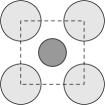
IH2
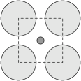
IH3
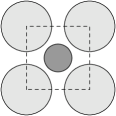
FH
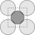
D
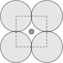
S
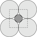
T
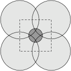
O
To have a finite horizon we must block horizontal, vertical and diagonal corridors. (The necessity to block diagonal corridors was overlooked in [Gar97].) Horizontal and vertical corridors are blocked by requiring the central disc to be sufficiently large, namely , and by symmetry it suffices to block diagonal trajectories at between mid-points of adjacent sides; for this the discs must be large enough. (If we instead use discs to block these diagonal trajectories, we necessarily have ; by our convention, we thus reduce to the case considered.) Hence for a finite horizon we supplement Garrido’s condition
| (3.3) |
with222Note that the critical case of a ‘grazing’ collision (when a trajectory is tangent to a scatterer) is sufficient to have normal diffusion.
| (3.4) |
The boundary between regions T and O occurs when the disc covers the whole region left empty between the overlapping discs. This occurs when the boundary of a disc reaches the point of intersection of the boundaries of two discs, when .
3.1.5 Channel geometry
Diffusion in a 2D infinite lattice is described by a second order diffusion tensor having components with respect to a given orthonormal basis, which we refer to as diffusion coefficients. If the system is sufficiently symmetric then the diffusion tensor reduces to a scalar multiple of the identity tensor. Square symmetry, as in the model presented above, and hexagonal symmetry, as in the standard triangular periodic Lorentz gas [KD00] are both sufficient for this reduction to occur; see also Sec. 3.6.
We study individually the components of the diffusion tensor, defined by
| (3.5) |
This enables us to check that and in fully symmetric systems. For those systems the diffusion coefficient can then be evaluated as an average over the multidimensional distribution via
| (3.6) |
as used e.g. in [KD00], but this cannot be applied to systems where the diffusion tensor is not a multiple of the identity tensor.
We can evaluate the diffusion coefficient by looking at the dynamics only in the -direction, which corresponds to studying the billiard dynamics in a -dimensional channel extended in the -direction; see Fig. 3.5. Correspondingly, we restrict attention to 1D marginal distributions, which are easier to analyse.

A channel geometry, with hard horizontal boundaries, corresponding to the triangular Lorentz gas was studied in [Gas93, AACG99] (Fig. 3.6). This is equivalent to a channel with twice the original height and periodic boundaries, by reflecting once in the hard boundary. This new channel is shown in Fig. 3.6 as part of the whole triangular lattice obtained by unfolding completely in the vertical direction. We can then view the triangular lattice as consisting of rectangular unit cells (Fig. 3.6) which are stretched versions of the square unit cell considered above, with the extra condition .


3.1.6 Effect of length scale on diffusion coefficient
Since we have two choices of length scale (Sec. 3.1.3), we need to know how to convert calculated diffusion coefficients between the two length scales. Recall the convention that , ; we also introduce for clarity .
Let be the position at time in the system with fixed and speed , with radii and ; and let be the position at time in the system with fixed and speed , with radii and .
The motion in the tilde system is then equivalent to that in the system, but with speed ; however, the size of the system is also shrunk by a factor . Thus we have
| (3.7) |
and so
| (3.8) |
Hence
| (3.9) |
where is the diffusion coefficient in the tilde system. (This result can also be obtained by dimensional analysis.)
3.2 Estimation of diffusion coefficient
Having set up the model, we now consider the statistical question of how to estimate the diffusion coefficient from numerical data.
3.2.1 Estimation of moments
A first approach to characterise the distribution of a random variable is to look at its moments. The th raw population moment of a random variable is given by333We follow the notation of [RS02].
| (3.10) |
where is the distribution function of the random variable ; the integral with respect to is a Lebesgue–Stieltjes integral, and the last equality holds if the random variable has a density .
If we take a sample of independent and identically distributed random variables from the distribution of , then the th sample raw moment is
| (3.11) |
This is an unbiased estimator of the th population raw moment , i.e. we have . Halmos [Hal46] showed that in fact it is the unique unbiased estimator of which is a symmetric function of the , and further that this estimator has the smallest variance of all unbiased estimators; in this sense it is the best estimator of given the sample.
We are mainly interested in the distribution of position and displacement in billiard models starting from an initial distribution which is uniform in a unit cell. By symmetry, the mean displacement then always vanishes, so that the simplest non-trivial characteristic of the distribution is the mean squared displacement444The notation emphasises that we are averaging over the distribution at time , but we have , where now we are thinking of averaging over the distribution of initial conditions. This distinction is the same as that between the Schrödinger and Heisenberg pictures in quantum mechanics. . We can view either as the 2nd raw moment of the random variable , or as the 1st moment of the distribution of the new random variable , as follows:
| (3.12) |
The best estimator of the mean squared displacement is thus
| (3.13) |
this can be regarded as a simple Monte Carlo estimator (see Sec. 2.6). In our numerical experiments we restrict ourselves to a fixed number of initial conditions , although in principle we could add more data until some pre-defined error tolerance was reached.
3.2.2 Distribution of mean squared displacement at time
To establish how good an estimator (3.13) is, we need to determine the width of the distribution of . The are independent and identically distributed (i.i.d.) random variables with mean ; since particles with speed satisfy , they also have finite variance. It follows that the are also i.i.d., with positive mean and finite variance. Hence the standard central limit theorem (Sec. 2.3.2) applies, so that for large the distribution of is very close to normal, with unknown mean and variance
| (3.14) |
For fixed , we thus arrive at the standard result that the width of the distribution of , as measured by the standard deviation (the square root of the variance) of , is .
The best estimator for this variance can be found using the known result for the variance of a sample mean, giving
| (3.15) |
3.2.3 Calculation of error bars: confidence interval for
We now establish a confidence interval for . For a normal random variable with mean and variance we have
| (3.16) |
i.e. the probability that a normal random variable lies within standard deviations of the mean is . Since neither nor are known for the distribution of , we estimate them via and , respectively, where is the value of for the data.
We will then estimate a confidence interval for by the interval estimator
| (3.17) |
Figure 3.7 shows the estimate as a function of for several samples. Error bars for one sample are also shown at ; the error bars contain most of the data for each sample.
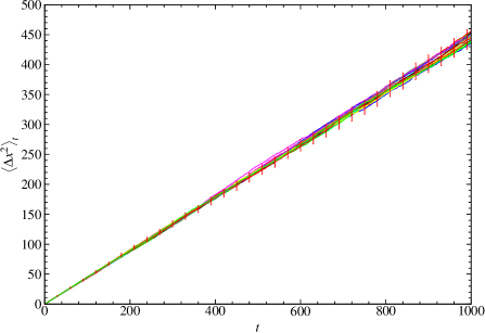
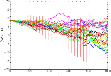
3.2.4 Estimation of diffusion coefficient
The most efficient method to estimate the diffusion coefficient is to use the fact that the asymptotic growth rate of the mean squared displacement in the linear regime is and to calculate this by fitting a straight line to the data in the presumed linear regime [KD00]. We must thus consider the evolution of over time. In practice, the linear regime is attained very rapidly: see Fig. 3.7(a). To find the slope in the asymptotic regime we apply linear regression (see e.g. [PTVF92]), performing a least squares fit of a straight line to the data in the region of large , making sure that the correlation coefficient of the fit is very close to .
The linear regression procedure gives an estimate of the diffusion coefficient as the slope of the fitted line. We also need to estimate the possible error that this estimate has made compared to the true value. This question is treated in statistics textbooks mostly for data whose errors are independent. This is however not the case here: if at a given time the estimated mean squared displacement has deviated from the ‘correct’ value, then at a small time later, there is a large probability that the mean squared displacement deviates away from the ‘correct’ value in the same direction as in the previous step.
3.2.5 Growth of width of distribution of with
To find the growth rate of the width of the distribution, we argue as follows. Since the distribution of at a fixed time is (approximately) normal, we only need to consider the standard deviation. We have
| (3.18) |
setting .
Chernov & Dettmann [CD00] showed that for a periodic Lorentz gas with finite horizon, the 4th-order Burnett coefficient exists, where
| (3.19) |
and
| (3.20) |
is the 4th-order cumulant555The set of cumulants of a distribution is an alternative set of moment-type descriptors of a distribution which have certain advantages over the raw moments: see e.g. [RS02]. For example, for independent random variables and ; this does not hold in general for .. This cumulant is related to the non-dimensional kurtosis excess via
| (3.21) |
the kurtosis excess is a common measure of how far a distribution is from a Gaussian, the difference being exactly for a Gaussian [Wei].
We thus have
| (3.22) |
since grows like whereas grows like . Hence the width of the distribution of , as measured by the standard deviation, grows like . This does not seem to have been previously remarked; it can be seen in Fig. 3.8, where the half-width of a confidence interval for is plotted as a function of .
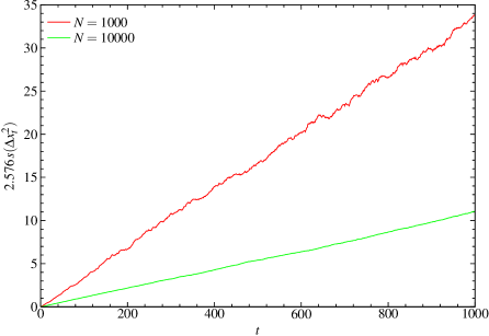
We note that Garrido & Gallavotti [GG94] considered the question of estimating the error in the diffusion coefficient by an expansion assuming that the errors are small. However, if we could continue the simulation indefinitely, the above calculation shows that the errors would grow arbitrarily large. Nonetheless we can still estimate an error in the diffusion coefficient, as follows.
3.2.6 Sampling distribution of diffusion coefficient
By repeating the above estimation procedure for different sets of random initial conditions, we obtain a sample set of estimated values of the diffusion coefficient. From these we can estimate the sampling distribution of ; this will indicate how close to the true underlying value of the estimate is expected to be.
Suppose that the confidence intervals for the mean squared displacement enclose all of the data. Then the growth rate of the data must lie between the rates of growth of the upper and lower limits of the error bars. In fact we can never guarantee that all the data is enclosed, but nonetheless we estimate the width of the distribution by fitting straight lines to the error bars. For confidence intervals on the mean squared displacement error bars, we would naively hope to obtain a confidence interval on . However, a confidence interval for each point does not necessarily correspond to a confidence band for the whole curve [Ric94].
We investigate the sampling distribution of by constructing a kernel density estimate [Sil86] of the sampling density. Fig. 3.9 shows the sampling density obtained for particular geometrical parameters for samples of size . For this case, the standard deviation of the sampling distribution is . The supposed confidence interval found by the above method (fitting upper and lower error bar limits) is . (This value varies depending on the sample.) The estimated error bars from hence correspond to a width of , which is approximately a confidence interval. Our method thus slightly underestimates the width of the sampling distribution. We have repeated the calculation for larger values of , and have found empirically that our method of estimating the width of the distribution improves as increases.
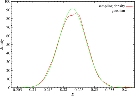
3.3 Geometry dependence of diffusion coefficients
We now consider the geometry-dependence of the diffusion coefficient in our model as a function of the geometrical parameters. This question has been studied in [KD00] for the triangular Lorentz gas, and in [HKG02] in a billiard with ‘flower-shaped’ scatterers. As emphasised above, our model has the advantage that we can vary independently two physical factors which we expect to influence the diffusion coefficient: (i) the size of trap exits; and (ii) the available area in each unit cell. We remark that striking results have also been obtained for lifted circle maps on the real line [KD95, GK02], where a fractal parameter dependence of the diffusion coefficient was found. This motivated a conjecture of Klages [KD00] that the diffusion coefficient in low-dimensional dynamical systems could in general be a highly non-trivial function of parameter666 [ Rigorous results on this question have recently been obtained for simple maps [KHK08] and Lorentz gases [CD, chapter 5].] . We have not attempted to address this question: although we find that the diffusion coefficient in our model is a reasonably smooth function of parameter, we have not studied the fine-scale dependence in detail.
3.3.1 Constant trap exit size
In this section we work in the tilde scaling, i.e. fixing the side of the unit cell to be of length . The parameters varied are then and .
We fix the radius of the non-central discs and vary the central disc radius over the allowed portion of the finite horizon regime for that value of . We repeat this for different values of covering the finite-horizon regime. Each curve thus corresponds to fixing the size of the exits of the unit cell, while the trap area varies. Figure 3.10(a) shows the diffusion coefficient over the whole finite-horizon regime. The curves are plotted over the allowed range
| (3.23) |
vanishes for , since the particle is then completely trapped in a bounded region, so the rightmost symbol on each curve is plotted at ,0). Error bars, estimated as in the previous section, are plotted, and are indistinguishable from the data symbols (except possibly for the largest values of ).

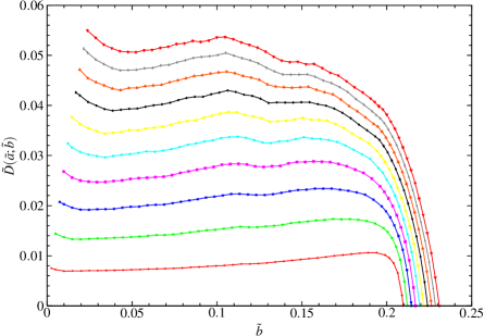
We note the following features of these graphs.
-
(i)
The curves seem to be continuous as a function of , with some degree of regularity.
-
(ii)
They possess features such as local minima and maxima which are reproduced in nearby curves, indicating that there is also continuity of as a function of with fixed (see also below).
-
(iii)
Decreasing with fixed results in faster diffusion.
- (iv)
-
(v)
For close to its upper bound , i.e. when the -discs are very close together, the maximum diffusion rate occurs for a value of close to .
Point (iii) corresponds to the findings with the triangular periodic Lorentz gas [KK02], since there both trap area and trap exit size increase when the parameter is increased. Intuitively, it is ‘easier’ for the particle to move through the lattice.
Point (iv) is reminiscent of the behaviour near to a critical point in the context of phase transitions. We have not found a physical explanation of this, although Sec. 3.4 contains some related comments.
Diffusion coefficient as function of gap size
Since the finite-horizon regime is a parallelogram, it is interesting to consider the diffusion coefficient in terms of a new variable giving the distance above the least allowed value for . In fact, we also have
| (3.24) |
where is the minimum distance from the boundary of the -disc to the boundary of an -disc (see also the next section). This is shown in 3.11. We can thus view the graph as plotting the diffusion coefficient as a function of this distance.
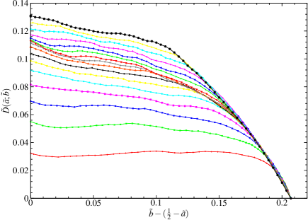
We see that the graphs approximately collapse for values of close to its maximum, i.e. when the - and -discs are close to touching. In particular, there seems to be a universal approach of the diffusion coefficient to when . We remark that it was shown in [Bun85] that viewing as a function of , we have
| (3.25) |
so that this approach occurs in a linear way as ; this should be contrasted, for example, with the square root-type behaviour often found in phase transitions.
3.3.2 Diffusion coefficient variation with constant trap area
We now fix the available area per unit cell and vary the trap exit size; again we work in the tilde system. Figure 3.12 shows the variation of the diffusion coefficient along circular curves in the parameter space of Fig. 3.2 with constant radius , and hence constant billiard domain area . The diffusion coefficient is plotted as a function of , the angle anti-clockwise from the -axis along the circle of radius . When we move along these circles the radius of the central disc increases, while the radius of the other discs decreases, and hence so does the trap exit size. We find the following:
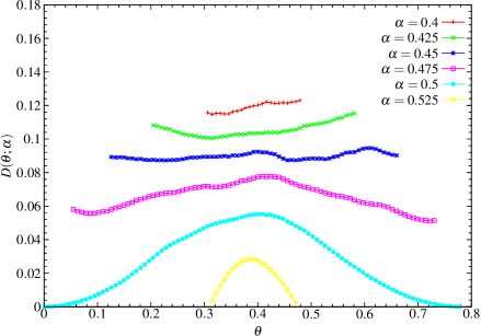
-
(i)
As decreases, and so the available area increases, the rate of diffusion increases.
-
(ii)
For larger values of , the curves lie mainly within two regions where a random walk model gives a good approximation to the diffusion coefficient, as we show in Sec. 3.4.
-
(iii)
For , the main effect seems to be due to variation of the trap area. However, there is a still some variation along the curves. This provides some evidence against the application of an approximation originating in the Boltzmann equation proposed in [KD00], since that approximation depends on density alone. In that paper the application was to the triangular periodic Lorentz gas, but the lack of variable parameters in that model did not allow the investigation of this question.
3.4 Machta–Zwanzig random walk model
We wish to understand the dependence of the diffusion coefficient on the geometry of the periodic Lorentz gas: can we predict the gross structure of curves such as those in Sec. 3.3 via analytical arguments? In this section we study the idea of Machta & Zwanzig [MZ83] to approximate the deterministic motion by a random walk.
3.4.1 Derivation of Machta–Zwanzig random walk approximation
The idea of Machta & Zwanzig [MZ83] is as follows. If the lattice spacing is such that the discs are very close, then the particle will on average be trapped for a long time in each unit cell. We refer to such a cell as a trap, where the exits of a trap should have a length which is small compared to its total perimeter. Due to the scattering nature of the boundaries, the velocity autocorrelation function decays fast, in fact exponentially in the number of collisions [CY00]. Thus when the particle leaves a trap, its motion will be almost uncorrelated with its motion on entering the trap. We thus try to approximate the deterministic motion by a completely uncorrelated random walk between traps.
Machta & Zwanzig gave a physical argument which enabled them to calculate the mean residence time in a trap. The result agrees with a rigorous calculation discussed below. Once the mean residence time is known, we can derive the diffusion coefficient of the random walk via
| (3.26) |
for a 2D random walk on an isotropic lattice with lattice spacing and residence time .
3.4.2 Application to our model
Let be the trap region and the part of its boundary (lying on the edge of the torus viewed as a square) which particles can cross, and denote by the -dimensional Lebesgue measure of the -dimensional set . Then by an argument detailed in Sec. 3.5.3, together with a method of Chernov (see [CM01, Che97]), we have
| (3.27) |
Here is the normalising constant for the measure introduced in Sec. 3.5.3 and is the normalising constant for the measure . Further, is the -dimensional unit ball and is its boundary, the -dimensional unit sphere. In 2D, we have and , so that
| (3.28) |
The exact expression (3.27) for the mean residence time is precisely analogous to the exact expression for the mean free path discussed in [Che97]; it also agrees with the more physical argument of [MZ83].
For the square Lorentz gas that we consider, there are two different regimes in which we can expect the Machta–Zwanzig method to be valid: see Fig. 3.13. In (a), the -discs are almost touching, so that the – gaps control the escape process from each trap. In (b), the -disc is so large that the – gap will now control the dynamics.


In regime (a) we have
| (3.29) |
and hence
| (3.30) |
whilst in regime (b), we have
| (3.31) |
and hence
| (3.32) |
Introducing the quantities
| (3.33) |
which are the the – and – gap sizes, respectively, we can summarize the above as
| (3.34) |
where the th approximation is expected to be valid when is small relative to the perimeter of a cell.
3.4.3 Comparison of Machta–Zwanzig approximation with data
Figure 3.14 and Fig. 3.15 show comparisons of the two Machta–Zwanzig approximations with numerical data for the diffusion coefficient as a function of and of , respectively, where is again the angle of the point in parameter space from the line . We see that the Machta–Zwanzig approximations are good when the respective are small, but fail elsewhere.
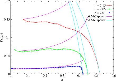
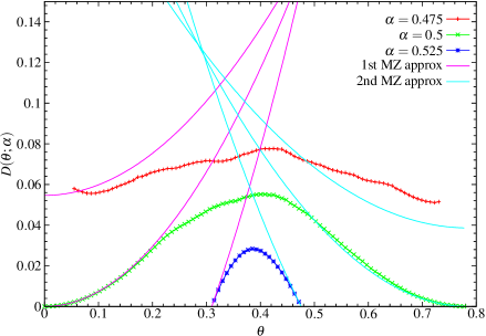
To some extent, these approximations explain the observation from Sec. 3.3 that there is a non-trivial maximum for values of near , since in that case the first approximation is valid for small and the second is valid for large , and they combine to predict a maximum at an intermediate value of . It is clear, however, that other effects are important in this intermediate regime.
For larger values of , decreasing has the effect of allowing the particles freer passage through the system, so intuition would again predict the observed increase in the diffusion coefficient on decreasing .
3.4.4 Trap residence time distribution
Since the above arguments involve the residence time , we here study numerically its distribution as a random variable, where . (The space and measure are discussed in more detail in Sec. 3.5.) To do this, we need to distribute particles uniformly with respect to the invariant measure on , i.e. on the trap exits with inward-pointing velocities. It is sufficient to distribute them uniformly with respect to Liouville measure in the billiard domain and evolve them forward until the first intersection with the trap exit boundary. By definition of the measure , they will then be correctly distributed.
We simulate the dynamics until the first exit from this trap and record the trap residence time, for an ensemble of particles. We then estimate the density of this distribution using a histogram. The results are shown in Fig. 3.16 for two different geometries.
An argument similar to that of Machta & Zwanzig, looking at the area available to escape in a small time , would imply an exponential distribution. However, there is a minimum trap residence time given by the time it takes to enter a trap in the centre of one of its sides with a velocity perpendicular to that side, collide with a -disc, and exit along the same path. This minimum time is thus . In Fig. 3.16 we thus compare the numerical distribution with an exponential distribution with density
| (3.35) |
with mean , and a delayed exponential distribution given by
| (3.36) |
where , both of which have mean . We see that the delayed exponential captures well the correct asymptotic behaviour, whereas the standard exponential does not.
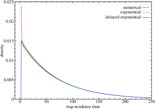
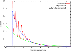
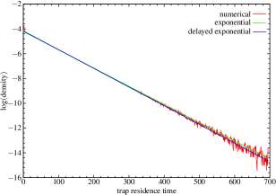
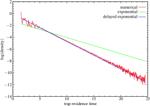
We remark that we can replace the simple Machta–Zwanzig approximation with an a priori more general one where we use a continuous-time random walk formulation with a (delayed) exponential residence time distribution. However, it turns out that we obtain the same result for the diffusion coefficient from any residence time distribution with a finite mean, as was already found in [Shl74]; see also [Wei94, Chap. 3], and Sec. 5.5 for further discussion of continuous-time random walk models.
3.5 Generalised random walk models and Green–Kubo approaches
Klages & Dellago [KD00] extended the Machta–Zwanzig approach in a heuristic way, by including the probability to follow specified sequences of traps. Klages & Korabel [KK02] then found a way to include such corrections in an exact Green–Kubo-type expansion. We believe, however, that while the result was correct, and the method was mostly correct, there is a gap in the justification, since the relationship between the discrete-time and continuous-time approaches studied above was not treated correctly. Here we show how to close the gap in the argument.
3.5.1 Original argument of Klages & Korabel [KK02]
In the appendix of [KK02], Klages & Korabel argued as follows. We wish to generalise the idea of a hopping process between traps, for which we must pass from the continuous-time expression for the diffusion coefficient in terms of the Einstein formula for a symmetric system,
| (3.37) |
to a formula in terms of some discrete time . The mean here is with respect to the invariant measure on the phase space of the flow.
To do this, Klages & Korabel [KK02] set777In [MZ83] and [KK02], denotes the average residence time in a trap. We follow the convention in the mathematical literature (e.g. [CM01]), where is used for the free path function, with mean . Denoting by the trap residence time function, we replace the of [KK02] by .
| (3.38) |
where is the random variable giving the position at time and is the position at the th step. Note that here the ‘th step’ simply means times the (so far arbitrarily chosen) time step . Then (3.37) implies that
| (3.39) |
where the mean is still with respect to .
Since we want an expression in terms of traps, we must show that we can replace by , the centre of the trap in which lies. Set , the displacement of the position at step from the centre of the respective trap. Then (3.37) implies that
| (3.40) |
where , assuming that all initial conditions are in the trap at . We expand
| (3.41) |
and note that the last term is bounded by , where is the diameter of a unit cell. The Cauchy–Schwarz inequality for the second term then gives
| (3.42) |
so that the second term grows only as fast as the square root of the first term. Hence we obtain
| (3.43) |
solely in terms of the trap at time .
The next step is to obtain a Green–Kubo formula in terms of the jump vector using the telescoping sum
| (3.44) |
where the equality follows since . This reduces exactly to the variance of a sum of stationary random variables, giving
| (3.45) |
so that
| (3.46) |
Thus if decays sufficiently fast as , then we can take the limit of (3.46) as to obtain the Green–Kubo relation
| (3.47) |
Klages & Korabel then use this result to try to extend the Machta–Zwanzig approximation, as follows. They follow each trajectory and record the sequence of traps visited via a symbol sequence. They numerically calculate the probability of occurrence of each symbol sequence and use sequences of length up to as an th-order approximation to the Green–Kubo expression, where the Machta–Zwanzig approximation can be regarded as the th-order approximation. They obtain results which numerically converge exactly to the (numerically) exact diffusion coefficient over the whole finite-horizon regime of the triangular Lorentz gas. The same method was applied in a different model in [HKG02].
3.5.2 Re-examination of Klages–Korabel derivation
We argue that the derivation given is not directly related to the numerical method subsequently employed, although both are independently correct. The reason for this is confusion in the definition of the th time step:
-
(i)
In the derivation, the th time step was taken as looking stroboscopically at the flow at the start of each period of length .
-
(ii)
In the numerical method, however, the th ‘time step’ instead refers to the time when the phase space point crosses into the th trap.
Both interpretations correspond to valid reductions from the continuous-time flow to a discrete-time map, but they are not equivalent: (i) corresponds to looking at statistical properties of the time- map of the flow, while we will show that (ii) corresponds instead to looking at statistical properties of a particular Poincaré map, which differs from the usual billiard map and which we call the torus-boundary map.
The part of the derivation after the definition of the position ‘at the th time step’, is valid in each case, and shows that in any of these cases it is equivalent to study the asymptotic behaviour either of or of the corresponding trap centre , or of the jump vectors defined as above, provided their correlations decay sufficiently fast. As far as we are aware, no rate of decay of correlations is yet available for the time- map (which would be related to the still-unsolved problem of the correlation decay rate for the billiard flow), nor for the torus-boundary map (which does not seem to have been studied previously).
3.5.3 Torus-boundary map
Analogously to the billiard map (which takes one collision with the scatterers to the next), we introduce a map , which we call the torus-boundary map, mapping one intersection with the trap/torus boundary to the next. Thus the domain of is
| (3.48) |
and we follow the trajectory up to the edge of the torus and then continue to the point on the opposite edge with which that point is identified.
The torus-boundary map will be undefined for phase points whose trajectories get trapped bouncing between the scatterers, i.e. for points on the stable manifold of the fractal repeller. However, this set has measure zero [Gas98], so that is defined almost everywhere.
We can now view the billiard flow as a suspension flow over the torus-boundary map , under the trap residence time function , since specifying a phase space point in and a value for the residence time function specifies a unique point of . The invariant measure on the space is defined analogously to the invariant measure for the billiard map , i.e. by projecting to , and then by App. B, is ergodic. Hence, by the Birkhoff ergodic theorem, for almost every , we have that
| (3.49) |
i.e. time averages of the residence time function are equal to , so that is indeed the mean trap residence time.
We can now use the relation between the variance of the suspension flow and the variance of the base transformation (see App. B) to get an expression for in terms of statistical properties of the base transformation. This reduces exactly to (3.39), where is the position at the th crossing of a trap boundary and the average is with respect to the invariant measure for the torus-boundary map.
The regularity of the roof function required for this result (see App. B) is satisfied, since the roof function, which is here given by the trap residence time function, appears to decay exponentially; this was shown numerically in Sec. 3.4.4, although we are not aware of any rigorous results.
The remainder of the above derivation of Klages–Korabel now goes through to give a Green–Kubo formula in terms of the torus-boundary map, provided that correlations decay sufficiently fast. As far as we are aware, the only results on decay of correlations for billiards are for the billiard map, where exponential decay of correlations is proved [You98, Che99, CY00]. We expect that correlations for the torus-boundary map also decay exponentially fast. However, the proofs for the billiard map rely on hyperbolicity due to the scattering nature of billiard boundaries. In the case of the torus-boundary map, the boundaries are not scattering: the scattering occurs between, rather than at, intersections with the boundary. It is thus possible that a rigorous proof could be even harder to obtain than for the billiard map. If we nonetheless assume that these correlations do decay sufficiently fast, we do have a Green–Kubo expansion such that the Machta–Zwanzig result occurs as the th order approximation. This completes the justification of the Klages–Korabel method.
We remark that this method extends to any other map such that we can express the billiard flow as a suspension over that map. However, we are not aware of other physically interesting maps for which that is the case.
3.5.4 Low-order approximations
If the details of the above justification can be made rigorous, we would then be able to rigorously assert that the Machta–Zwanzig approximation is indeed a zeroth-order truncation of the infinite Green–Kubo sum. In [KK02], it was observed that a certain simple low-order expression involving collisionless flights across traps gave a very good approximation of the numerical diffusion coefficient over the whole finite horizon regime for the triangular Lorentz gas. This was an anomaly from the point of view of the expansion used in that paper, since this truncation did not appear explicitly in the Green–Kubo sum used there.
We believe that this anomaly can be explained by noting that their expression was instead a natural low-order truncation of the discrete-time Green–Kubo formula obtained from the time- map, rather than from the torus-boundary map: there we must include in the first term a sum over all accessible traps after a time , which includes at least part of the probability of collisionless flights, together with part of the backscattering probability which also appears in their best low-order truncation. Their observation then suggests that the Green–Kubo expression discussed above converges more rapidly as the truncation order increases than that used in their paper. This faster rate of convergence depends on correlations for the two respective maps; as such, we would not expect to be able to predict which of the two expansions would give better low-order approximations without a detailed knowledge of these correlations.
3.6 Reducing the geometrical symmetry
In this section we study the effect of altering the geometry of the system to reduce the symmetry of the unit cells; again our model is a good candidate for this, whereas the triangular model would perhaps be less natural.
3.6.1 Symmetry of diffusion tensor
We first consider the effect of symmetry on the diffusion tensor. Suppose we measure the diffusion coefficients in the original coordinate system and in a new orthonormal coordinate system based at the same origin, given by , where is the orthonormal change of basis matrix (i.e. a combination of rotations and reflections). Then the diffusion coefficients with respect to the new axes are given by
| (3.50) |
where we have used the Einstein summation convention (sum over repeated indices). If the system is symmetric under some symmetry element , then for that particular we have , since the system looks the same after the transformation. We remark that this idea is known as Neumann’s principle in the literature on crystal properties [Nye85], where it is an empirically based fact. In our setting, however, it is a theorem, since Liouville measure is invariant under the point group of the lattice.
Thus symmetry under the transformation implies that the diffusion tensor satisfies
| (3.51) |
This equation in general restricts the allowed values of the diffusion coefficient. For example, if the system is unchanged under reflection in the -axis, given by the transformation having matrix
| (3.52) |
then we find that (3.51) implies that for a 2D system, so that the diffusion tensor is diagonal in this coordinate system. In the case of 3D systems (which we have not investigated), tables of crystal symmetries and their consequences for possible forms of the 2nd-order diffusion tensor can be found e.g. in [CJ88, Nye85].
3.6.2 Displacing central disc
Here we consider the effect of displacing the -discs away from the centre of the cell888I would like to thank Leonid Bunimovich for suggesting this, with the idea that it could help to understand the validity of the Machta–Zwanzig approximation., parallel to the -axis. Then the system remains symmetric under reflection in the -axis, but is now asymmetric under reflection in the -axis. By the above, the diffusion tensor must remain diagonal, but we may now have , which is not possible for the square model.
Starting from geometrical parameters lying in the finite horizon regime, we displace the -disc by a distance along the -axis in the direction of increasing . To continue to block the central vertical channel, we cannot move the -disc too far: we require , i.e.
| (3.53) |
The -disc touches the -discs when
| (3.54) |
so that the discs are not touching when
| (3.55) |
It is possible that there is a finite horizon even if the - and -discs touch. In this case, there is no possibility for the particle to escape from the vertical channel in which it begins, so that ; however, there may still be a non-trivial diffusion coefficient in the -direction. Note, however, that the analysis of [BS81, BSC91] does not immediately apply to this case, since the (convex) scatterers are no longer disjoint.
Figure 3.17 shows numerical data for the diffusion coefficients and for this system as a function of the displacement . For , we have by the symmetry results above. For non-zero , however, decreases and increases.
Increasing past the point where the discs touch, the area available in each cell increases; from the figure we see that suddenly increases its growth rate for two of the three sets of geometrical parameters studied.
On the contrary, for the value of seems to stabilise for larger values of , indicating some kind of balance between the increased phase space volume available and the control of the dynamics by the small trap exits.
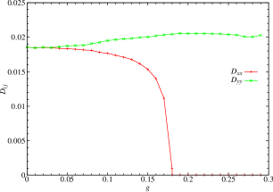
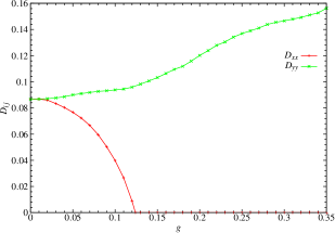
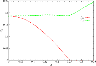
3.6.3 Rectangular model with less symmetry
We could also stretch the unit cell to a rectangular one, imposing different lattice spacings in the horizontal and vertical directions; this introduces two new geometrical parameters. In particular, the standard triangular periodic Lorentz gas can be considered as a particular case of such a stretched model. Again the symmetry of the diffusion tensor will be reduced in general, although not in the special case of the triangular periodic Lorentz gas.
Chapter 4 Fine structure of distributions and the central limit theorem in 2D periodic Lorentz gases
In the previous chapter we studied the statistical properties of the displacement as a function of time in terms of means. Those means are taken over the probability distribution of the observable, whose shape we investigate in this chapter.
As described in Chap. 2, it was proved in [BS81, BSC91] that 2D periodic Lorentz gases with finite horizon and disjoint scatterers (with sufficient smoothness of the scatterer boundaries, namely piecewise ) satisfy a central limit theorem: the rescaled displacement distribution converges in distribution to a limiting normal distribution:
| (4.1) |
In this chapter we study the structure of position and displacement distributions at finite time . We show that they possess a fine structure, consisting of a periodic oscillation superimposed on the Gaussian shape that we expect from a diffusive process. We will find an analytical description of this fine structure in terms of the geometry of the billiard domain, and provide extensive numerical evidence that this is indeed the main influence on the fine structure. This gives a physical picture of the weak type of convergence occurring in (4.1), and leads to a conjecture on a possible stronger result; we can also give an intuitive estimate of the rate of convergence to the limiting distribution.
The results in [BS81, BSC91] show how we can smooth away the fine structure to obtain rigorous proofs of convergence. Our analysis reinstates the fine structure to give a picture of how this convergence occurs, making explicit the obstruction that prevents a stronger form of convergence to the limiting normal distribution by showing how density functions fail to converge pointwise to Gaussian densities.
4.1 Structure of 2D position and displacement distributions
4.1.1 Statistical properties of position and displacement distribution
The displacement distribution occurs naturally in the central limit theorem (Sec. 2.3) and in Green–Kubo relations [Dor99, Gas98], whereas the position distribution is more natural if we are unable to track the paths of individual particles. Their statistical properties are very closely related, as shown by the following discussion for the -component.
Expanding the mean squared displacement as
| (4.2) |
and applying the Cauchy–Schwarz inequality to the second term on the right hand side, as in [KK02], which gives
| (4.3) |
we see that and have the same asymptotic growth rate, so that they both grow linearly if one of them does.
Further, since , we can show that the -rescaled position distribution also satisfies the central limit theorem if the displacement distribution does, with the same limiting normal distribution. From the point of view of statistical properties it is hence equivalent to study either the position or the displacement distribution.
4.1.2 Shape of 2D distributions
Figure 4.1 shows scatterplots representing 2D position and displacement distributions for a representative choice of geometrical parameters. Each dot represents one initial condition started in the central unit cell and evolved for time ; samples are shown, started from random initial conditions distributed uniformly with respect to Liouville measure in the central unit cell. Both distributions show decay away from a maximum in the central cell, an overall circular shape, and the occurrence of a periodic fine structure.
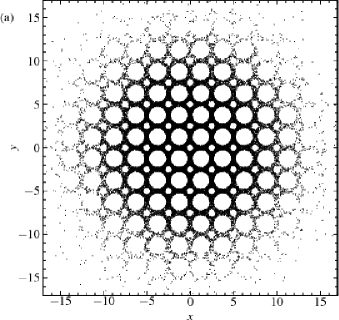
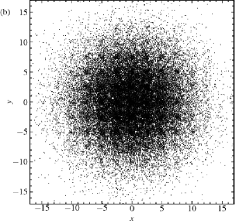
These figures are projections to the unfolded billiard domain of the density in the unfolded phase space . Since the dynamics on the torus is mixing [CM01], the phase space density converges weakly [LM94] to a uniform density on phase space corresponding to the invariant Liouville measure: see App. C. Physically, the phase space density on the torus develops a complicated layer structure in the stable direction of the dynamics: see e.g. [Dor99]. Projecting corresponds to integrating over the velocities; we expect this to eliminate this complicated structure and result in some degree of smoothness of the projected densities on the torus, and so presumably also of the unfolded projected densities. However, we are not aware of any rigorous results in this direction, even for relatively well-understood systems such as the Arnold cat map [Dor99].
These 2D distributions are difficult to work with, and we instead restrict attention to one-dimensional marginal distributions, i.e. projections onto the -axis, which will also have some degree of smoothness. We denote the 1D position density at time and position by and the displacement density for displacement by . We let their respective (cumulative) distribution functions111Henceforth we use ‘distribution function’, eliminating the redundant ‘cumulative’: this seems to be the usual terminology in probability theory, e.g. [GS92, Fel71]. be and , respectively, so that
| (4.4) |
and similarly for . (When necessary, we will instead denote displacements by .) The densities show the structure of the distributions more clearly, while the distribution functions are more directly related to analytical considerations.
4.2 Numerical estimation of 1D distribution functions and densities
We wish to estimate numerically the above densities and distribution functions at time from the data points . The most widely used method in the physics community for estimating density functions from numerical data is the histogram [PTVF92]. However, histograms are not always appropriate, due to their non-smoothness and dependence on bin width and position of bin origin [Sil86]. In [ARdV02], for example, the choice of a coarse bin width obscured the fine structure of the distributions that we describe in Chap. 5.
We have chosen the following alternative method, which seems to work well in our situation, since it is able to deal with strongly peaked densities more easily, although we do not have any rigorous results to justify this. We have also checked that histograms and kernel density estimates (a generalization of the histogram [Sil86]) give similar results, provided that sufficient care is taken with bin widths.
We first calculate the empirical cumulative distribution function [Sco92, Sil86], defined by for the position distribution, and analogously for the displacement distribution. The estimator is the optimal one for the distribution function given the data, in the sense that there are no other unbiased estimators with smaller variance [Sco92, p. 34]. We find that the distribution functions in our models are smooth on a scale larger that that of individual data points, where statistical noise dominates. (Here we use ‘smooth’ in a visual, nontechnical sense; this corresponds to some degree of differentiability). We verify that adding more data does not qualitatively change this larger-scale structure: with samples we seem to capture the fine structure.
We now wish to construct the density function . Since the direct numerical derivative of is useless due to statistical noise, our procedure is to fit an (interpolating) cubic spline to an evenly-spread sample of points from , and differentiate the cubic spline to obtain the density function at as many points as required. Sampling evenly from automatically uses more samples where the data are more highly concentrated, i.e. where the density is larger.
We must confirm (visually or in a suitable norm) that our spline approximation reproduces the fine structure of the distribution function sufficiently well, whilst ignoring the variation due to noise on a very small scale. As with any density estimation method, we have thus made an assumption of smoothness [Sil86]. The analysis of the fine structure in Sec. 4.1 justifies this to some extent.
4.3 Time evolution of 1D distributions
Figure 4.2 shows the time evolution of 1D displacement distribution functions and densities for certain geometrical parameters, chosen to emphasise the oscillatory structure. Other parameters within the finite horizon regime give qualitatively similar behaviour.
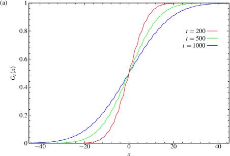
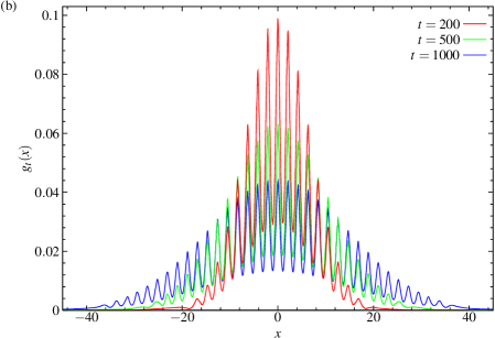
The distribution functions are smooth, but have a step-like structure. Differentiating the spline approximations to these distribution functions gives densities which have an underlying Gaussian-like shape, modulated by a pronounced fine structure which persists at all times (Fig. 4.2(b)). This fine structure is just noticeable in Figs. 4 and 5 of [ARdV02], but otherwise does not seem to have been reported previously, although in the context of iterated 1D maps a fine structure was found, the origin of which is related to pruning effects: see e.g. Fig. 3.1 of [Kla96]. We will show that in billiards this fine structure can be understood by considering the geometry of the billiard domain.
4.4 Fine structure of position density
Since Liouville measure on the torus is invariant, if the initial distribution is uniform with respect to Liouville measure, then the distribution at any time is still uniform. Integrating over the velocities, the position distribution at time is hence always uniform with respect to Lebesgue measure in the billiard domain , which we normalize such that the measure of is . Denote the two-dimensional position density on the torus at by . Then
| (4.5) |
Here, is the set of allowed values for particles with horizontal coordinate (see Fig. 4.3), and is the indicator function of the (one- or two-dimensional) set , given by
| (4.6) |
Thus for fixed , is independent of within the available space .
Now unfold the dynamics onto a 1-dimensional channel in the -direction, as in Fig. 3.5, and consider the torus as the distinguished unit cell at the origin. Fix a vertical line with horizontal coordinate in this cell, and consider its periodic translates along the channel, where . Denoting the density there by , we have that for all and for all and ,
| (4.7) |
We expect that after a sufficiently long time, the distribution within cell will look like the distribution on the torus, modulated by a slowly-varying function of . In particular, we expect that the 2D position density will become asymptotically uniform in within at long times.
We have not been able to prove this, but we have checked by constructing 2D kernel density estimates [Sil86] that it seems to be true. A ‘sufficiently long’ time would be one which is much longer than the time scale for the diffusion process to cross one unit cell. It does not, however, hold for short times: for example, in Fig. 4.4 we see the development of the 2D density at the leading edge. At the earlier time, we see that the ‘fluid’ has streamed past the small disc without reaching the region below it; at the later time, this region is beginning to be occupied. At long times, the mixing property of the dynamics will have filled the region approximately uniformly.
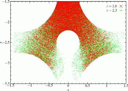
Thus we have approximately
| (4.8) |
where is the shape of the two-dimensional density distribution as a function of ; we expect this to be a slowly-varying function. We use ‘’ to denote that this relationship holds in the long-time limit, for values of which do not lie in the tails of the distribution. Although this breaks down in the tails, the density is in any case small there.
The 1D marginal density that we measure will then be given by
| (4.9) |
where is the normalized height (Lebesgue measure) of the set at position (see Fig. 4.3). Note that is not necessarily a connected set.
Thus the measured density is given by the shape of the 2D density, modulated by fine-scale oscillations due to the geometry of the lattice and described by , which we call the fine structure function.
The above argument motivates the (re-)definition of so that with strict equality and for all times, by setting
| (4.10) |
We can now view as the density with respect to a new underlying measure , where is -dimensional Lebesgue measure; this measure takes into account the available space, and is hence more natural in this problem (see also Sec. C.4). We expect that will now describe the large-scale shape of the density, at least for long times and comparatively small.
The conjecture underlying the above heuristic argument is then that for all , we have
| (4.11) |
or equivalently
| (4.12) |
where the ratio converges to something which is independent of . We must use this expression since the density at any fixed tends to as . In fact, regarding both sides as a function of , we could even expect uniform convergence of the form
| (4.13) |
where is still fixed.
Figure 4.5 shows the original and demodulated densities and for a representative choice of geometrical parameters. The fine structure in is very pronounced, but is eliminated nearly completely when demodulated by dividing by the fine structure , leaving a demodulated density which is close to the Gaussian density with variance (also shown).
Note that although the density has non-smooth points, which affects the smoothness assumption in our density estimation procedure described in Sec. 4.2, in practice these points are still handled reasonably well. If necessary, we could treat these points more carefully, by suitable choices of partition points in that method.
We estimated the diffusion coefficient as follows. For and , using particles evolved to , the best fit line for against in the region gives , which we regard as confirmation of asymptotic linear growth. Following [KD00], we use the slope of against in that region as an estimate of , giving ; the error analysis is as in Chap. 3. (Throughout, we denote by the Gaussian density with mean and variance , and by the corresponding normal distribution function.)
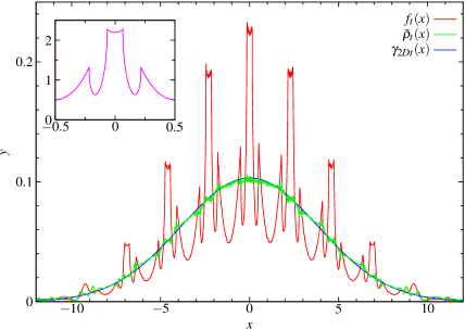
4.5 Fine structure of displacement density
We can treat the displacement density similarly, as follows. Let be the 2D displacement density function at time , so that
| (4.14) |
(Recall that .) We define the projected versions and as follows:
| (4.15) | |||
| (4.16) |
Again we view the torus as the unit cell at the origin where all initial conditions are placed. Note that projecting the displacement distribution on to the channel or torus gives the same result as first projecting and then obtaining the displacement distribution in the reduced geometry. Hence the designations as being associated with the channel or torus are appropriate.
Unlike in the previous section, is not independent of : for example, for small enough , all displacements increase with time. However, we show that rapidly approaches a distribution which is stationary in time.
Consider a small ball of initial conditions of positive Liouville measure around a point . Since the system is mixing on the torus, the position distribution at time corresponding to those initial conditions converges as to a distribution which is uniform with respect to Lebesgue measure in the billiard domain . The corresponding limiting displacement distribution is hence obtained by averaging the displacement of from all points on the torus.
Extending this to an initial distribution which is uniform with respect to Liouville measure over the whole phase space, we see that the limiting displacement distribution is given by averaging displacements of two points in , with both points distributed uniformly with respect to Lebesgue measure on . This limiting distribution we denote by , with no subscript.
As in the previous section, we expect the -dependence of to be the same, for large enough , as that of for . However, is not independent of , as can be seen from Fig. 4.6, which is a projected version of Fig. 4.1(b) to the torus (with different geometrical parameters). We thus expect
| (4.17) |
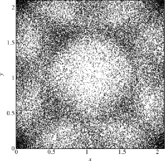
To obtain the 1D marginal density , we integrate with respect to :
| (4.18) |
where
| (4.19) |
Again we now redefine so that , with the fine structure of being described by and the large-scale variation by , which can be regarded as the density with respect to the new measure taking account of the excluded volume. In the next section we evaluate explicitly.
4.5.1 Calculation of -displacement density on torus
Let and be independent random variables, distributed uniformly with respect to Lebesgue measure in the billiard domain , and let be their -displacement, where denotes the fractional part of its argument. Then is the sum of two independent random variables, so that its density is given by the following convolution, which correctly takes account of the periodicity of and with period :
| (4.20) |
This form leads us to expand in Fourier series:
| (4.21) |
and similarly for , where the Fourier coefficients are defined by
| (4.22) |
The last equality follows from the evenness of , and shows that , from which the second equality in (4.21) follows. Fourier transforming (4.20) then gives
| (4.23) |
Taking the origin in the centre of the disc of radius (see Fig. 4.3), the available space function is given by
| (4.24) |
for , and is even and periodic with period . (Here we adopt the convention that if to avoid writing indicator functions explicitly.) The evaluation of the Fourier coefficients of thus involves integrals of the form
| (4.25) |
where is the first order Bessel function; this equality follows from equation (9.1.20) of [AS70] after a change of variables.
The Fourier coefficients of are thus and, for integer ,
| (4.26) |
Note that , so that is correctly normalized as a density function on the torus.
In Fig. 4.7 we plot partial sums up to terms of the Fourier series for analogous to (4.21). We can determine the degree of smoothness of , and hence presumably of , as follows. The asymptotic expansion of for large real (equation (9.2.1) of [AS70]),
| (4.27) |
shows that and hence . From the theory of Fourier series (see e.g. [Kat04, Chap. 1]), we hence have that is at least (once continuously differentiable). Thus the convolution of with itself is smoother than the original function, despite the non-differentiable points of .
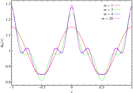
We have checked numerically the approach of to , and it appears to be fast, although the rate is difficult to evaluate, since a large number of initial conditions are required for the numerically calculated distribution function to approach closely the limiting distribution.
4.5.2 Structure of displacement distribution
In Fig. 4.8 we plot the numerically-obtained displacement density , the fine structure function calculated above, and their ratio , for a certain choice of geometrical parameters. Again the ratio is approximately Gaussian, which confirms that the densities can be regarded as a Gaussian shape modulated by the fine structure .
However, if is close to , then itself develops a type of fine structure: it is nearly constant over each unit cell. This is shown in Fig. 4.9 for two different times. We plot both and , rescaled by and compared to a Gaussian of variance . (This scaling is discussed in Sec. 4.6.)
This step-like structure of is related to the validity of the Machta–Zwanzig random walk approximation discussed in Sec. 3.4. Having constant across each cell indicates that the distribution of particles within the billiard domain in each cell is uniform, as is needed for the Machta–Zwanzig approximation to work.
As increases away from , the exit size of the traps increases, and the Machta–Zwanzig argument ceases to give a good approximation. The distribution then ceases to be uniform in each cell: see Fig. 4.5. This may be related to the crossover to a Boltzmann regime described in [KD00].
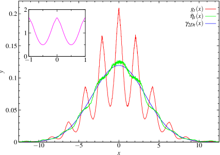
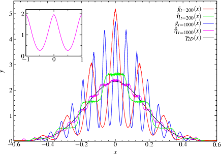
4.5.3 Comparison of position and displacement distributions
For long times, both position and displacement distributions converge to the same limiting normal distribution, so we expect the demodulated position and displacement distributions at a large but finite time to be close. This is confirmed in Fig. 4.10.
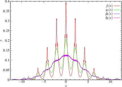
We can ask if there is in general any advantage in studying one or the other of the position and displacement distributions. Since , the Fourier coefficients of decay faster as than those of . This translates to better regularity (smoothness) of than of , as we have seen in the particular example above, where222 is Hölder continuous with exponent , denoted , if and only if . but .
Further, the convolution reduces the amplitude of the oscillations of the fine structure. We can see this by taking the first Fourier coefficient alone as an initial indication of the amplitude, putting
| (4.28) |
although there may be significant contributions to the amplitude from higher Fourier coefficients, as can be seen in Fig. 4.7. The first term ensures that is a density (per unit length), i.e. that integrates to , and is the amplitude of the oscillation. Then
| (4.29) |
so that the amplitude of the oscillations in (the lowest-order Fourier approximation of) is . If then the channel would have height at some point and no particle could pass. So the ratio of the amplitude of to that of is . This argument leads us to expect that indeed the amplitude of fine structure oscillations for the displacement density should be significantly less than that for the position density.
The above two results indicate that in numerical investigations it is more useful to concentrate on the displacement density, since we expect better performance of density estimation methods when the densities are smoother and less oscillatory.
4.6 Central limit theorem and rate of convergence
We now discuss the central limit theorem as in terms of the fine structure described in the previous section.
4.6.1 Central limit theorem: weak convergence to normal distribution
The central limit theorem requires us to consider the densities scaled by , so we define the rescaled densities
| (4.30) |
where the first factor of normalizes the integral of to , giving a probability density. Figure 4.11 shows the densities of Fig. 4.2(a) rescaled in this way, compared to a Gaussian density with mean and variance . We see that the rescaled densities oscillate within an envelope which remains approximately constant, but with an increasing frequency as ; they are oscillating around the limiting Gaussian, but do not converge to it pointwise. See also Fig. 4.9.
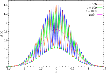
The increasingly rapid oscillations do, however, cancel out when we consider the rescaled distribution functions, given by the integral of the rescaled density functions:
| (4.31) |
Figure 4.12 shows the difference between the rescaled distribution functions and the limiting normal distribution with mean and variance . We see that the rescaled distribution functions do converge to the limiting normal, in fact uniformly, as ; we thus have only weak convergence of the distributions.
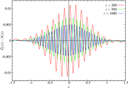
Although this is the strongest kind of convergence we can obtain for the densities with respect to Lebesgue measure, Fig. 4.9 provides evidence for the following conjecture: the rescaled densities with respect to the new measure converge uniformly to a Gaussian density. This characterizes the asymptotic behaviour more precisely than the standard central limit theorem.
4.6.2 Rate of convergence
Since the converge uniformly to the limiting normal distribution, we can consider the distance , where we define the uniform norm by
| (4.32) |
We denote by the normal distribution function with variance , given by
| (4.33) |
Figure 4.13 shows a log–log plot of this distance against time, calculated numerically from the full distribution functions. We see that the convergence follows a power law
| (4.34) |
with a fit to the data for giving a slope . The same decay rate is obtained for a range of other geometrical parameters, although the quality of the data deteriorates for larger , reflecting the fact that diffusion is faster, so that the distribution spreads further in the same time. Since we use the same number of initial conditions, there is a lower resolution near where, as shown in the next section, the maximum is obtained.
In [Pèn02] it was proved rigorously that for any Hölder continuous observable . Here we have considered only the particular Hölder observable , but for this function we see that the rate of convergence is much faster than the lower bound proved in [Pèn02].
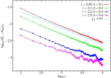
4.6.3 Analytical estimate of rate of convergence
We now show how to obtain a simple analytical estimate of the rate of convergence using the fine structure calculations in Sec. 4.4.
Since the displacement distribution is symmetric, we have for all . The maximum deviation of from occurs near to , where the density function is furthest from a Gaussian, while the fine structure of the density means that is increasing there (Fig. 4.12). Due to the oscillatory nature of the fine structure, this maximum thus occurs at a distance of of the period of oscillation from .
Since the displacement density has the form , after rescaling we have
| (4.35) |
where is the rescaled slowly-varying part of , and the fine structure at time is given by
| (4.36) |
The maximum deviation occurs at of the period of , i.e. at , so that
| (4.37) | ||||
| (4.38) |
The correction due to the curvature of the underlying Gaussian converges to as , since this Gaussian is flat at . Hence .
This calculation shows that the fastest possible convergence is a power law with exponent , and provides an intuitive reason why this is the case. This should be compared to the rate for convergence of rescaled distribution functions corresponding to solutions of the diffusion equation in App. A. If the rescaled shape function converges to a Gaussian shape at a rate slower than , then the overall rate of convergence could be slower than . However, the numerical results in Sec. 4.6.2 show that the rate is close to . We remark that for an observable which is not so intimately related to the geometrical structure of the lattice, the fine structure will in general be more complicated, and the above argument may no longer hold.
4.7 Maxwellian velocity distribution
In this section we consider the effect of a non-constant distribution of particle speeds333I would like to thank Hernán Larralde for posing this question, and for the observation that the resulting position distribution may no longer be Gaussian.. A Maxwellian (Gaussian) velocity distribution was used in polygonal and Lorentz channels in [LCW03] and [AACG99], respectively, in connection with heat conduction studies. The mean squared displacement was observed to grow asymptotically linearly, but the relationship with the unit speed situation was not discussed.
We show that the mean squared displacement grows asymptotically linearly in time with the same diffusion coefficient as for the unit speed case, but that the limiting position distribution may be non-Gaussian. For brevity we refer only to the position distribution throughout this section; the displacement distribution is similar.
4.7.1 Mean squared displacement
Consider a particle located initially at , where has unit speed. Changing the speed of the particle does not change the path it follows, but only the distance along the path traveled in a given time. Denoting by the billiard flow with speed starting from and with initial velocity in the direction of the unit vector , we have
| (4.39) |
where the flow on the right hand side is the original unit-speed flow. If all speeds are equal to , then the radially symmetric 2D position probability density after a long time is thus
| (4.40) |
giving a radial density
| (4.41) |
(Throughout this calculation we neglect any fine structure.)
If we now have a distribution of velocities with density , then the radial position density at distance is
| (4.42) |
The variance of the position distribution is then given by
| (4.43) | ||||
| (4.44) |
where is the mean speed, after interchanging the integrals over and .
We thus see that for any speed distribution having a finite mean, the variance of the position distribution, and hence the mean squared displacement, grows asymptotically linearly with the same diffusion coefficient as for the uniform speed distribution, having normalized such that . We have verified this numerically with a Gaussian velocity distribution: the mean squared displacement is indistinguishable from the unit speed case even after very short times.
4.7.2 Gaussian velocity distribution
Henceforth attention is restricted to the case of a Gaussian velocity distribution. For each initial condition, we generate two independent normally-distributed random variables and with mean and variance using the standard Box–Muller algorithm [PTVF92], and then multiply by , which is a standard deviation calculated below. We use and as the components of the velocity vector , whose probability density is hence given by
| (4.45) |
where is the speed of the particle. The speed thus has density
| (4.46) |
and mean . To compare with the unit speed distribution we require , and hence . As before, we distribute the initial positions uniformly with respect to Lebesgue measure in the billiard domain .
4.7.3 Shape of limiting distribution
The position density (4.42) is a function of time. However, the Gaussian assumption used to derive that equation is valid in the limit when , so the central limit theorem rescaling
| (4.47) |
eliminates the time dependence in (4.42), giving the following shape for the limiting radial density:
| (4.48) |
denoting the integral by . We can evaluate this integral explicitly using Mathematica [Wol04] in terms of the Meijer -function444The Meijer -function is a generalisation of the classical Gauss hypergeometric function, defined as the following Mellin–Barnes-type integral; for more details see [EMOT53, MS73, MK00]: (4.49) (4.50) is a certain contour in the complex plane and there are restrictions on the and the . [EMOT53, MS73]:
| (4.51) |
See [MK00] and references therein for a review of the use of such special functions in anomalous diffusion.
We can, however, obtain an asymptotic approximation to from its definition as an integral, without using any properties of special functions, as follows. Define , the negative of the argument of the exponential in (4.48). Then has a unique minimum at and we expect the integral to be dominated by the neighborhood of this minimum. However, the use of standard asymptotic methods is complicated by the fact that as , tends to , a boundary of the integration domain.
To overcome this, we change variables to fix the minimum away from the domain boundaries, setting . Then
| (4.52) |
where and , with a minimum at . Laplace’s method (see e.g. [CKP66]) can now be applied, giving the asymptotic approximation
| (4.53) |
valid for large , i.e. for large .
Hence
| (4.54) |
where
| (4.55) |
4.7.4 Comparison with numerical results
Figure 4.14 shows the numerical radial position density for a particular choice of geometrical parameters. We wish to demodulate this as in Sec. 4.1 to extract the slowly-varying shape function, which we can then compare to the analytical calculation.
The radial fine structure function must be calculated numerically, since no analytical expression is available. We do this by distributing points uniformly on a circle of radius and calculating the proportion of points not falling inside any scatterer. This we normalize so that as , using the fact that when is large, the density inside the circle of radius converges to the ratio of available area per unit cell to total area per unit cell. We can then demodulate by , setting
| (4.56) |
Figure 4.14 shows the demodulated radial density at two times compared to the exact solution (4.48)–(4.51), the asymptotic approximation (4.54)–(4.55), and the radial Gaussian . The asymptotic approximation agrees well with the exact solution except at the peak, while the numerically determined demodulated densities agree with the exact long-time solution over the whole range of . All three differ significantly from the Gaussian, even in the tails. We conclude that the radial position distribution is non-Gaussian. A similar calculation could be done for the radial displacement distribution, but a numerical integration would be required to evaluate the relevant fine structure function.
An explanation of the non-Gaussian shape comes by considering slow particles which remain close to the origin for a long time, and fast particles which can travel further than those with unit speed. The combined effect skews the resulting distribution in a way which depends on the relative weights of slow and fast particles.
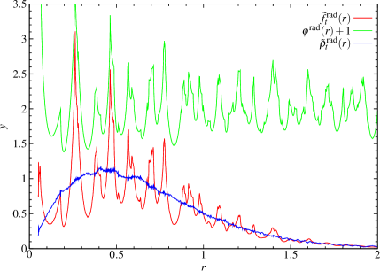
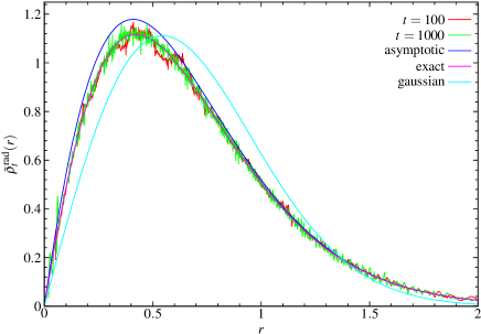
4.7.5 1D marginal
The 1D marginal in the -direction is shown in Fig. 4.16. Again there is a significant deviation of the demodulated density from a Gaussian. From (4.54), the 2D density at is asymptotically
| (4.57) |
from which the 1D marginal is obtained by
| (4.58) |
It does not seem to be possible to perform this integration explicitly for either the asymptotic expression (4.57) or the corresponding exact solution in terms of the Meijer -function. Instead we perform another asymptotic approximation starting, from the asymptotic expression (4.57). Changing variables in (4.58) to and using the evenness in gives
| (4.59) |
where . Laplace’s method then gives
| (4.60) |
valid for large . This is also shown in Fig. 4.16. Due to the factor, the behaviour near is wrong, but in the tails there is reasonably good agreement with the numerical results.
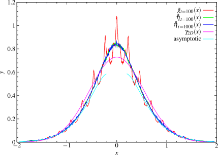
Chapter 5 Normal and anomalous diffusion in polygonal billiard channels
5.1 Introduction: ergodic and statistical properties in polygonal billiards
The rigorous results on statistical properties of Lorentz gases discussed in Chap. 2 depend on the hyperbolicity of the dynamics due to the defocusing nature of the scatterers. Recently the question has been asked to what extent hyperbolicity is actually necessary (rather than just sufficient) for these strong statistical properties to hold [DCv99, DC01].
The weak nature of the scattering from flat obstacles implies that in polygonal billiards the Kolmogorov–Sinai entropy and all Lyapunov exponents are , so that infinitesimally separated trajectories separate slower than exponentially; in fact they separate linearly, as can be seen by unfolding the polygonal billard and considering two initial conditions with slightly different angles. Nonetheless, trajectories separated by a finite distance may fall on different sides of a polygonal vertex, causing them to separate faster. Characterising this effect is difficult: see e.g. [vB04] for a recent attempt.
If all angles are rational, i.e. rational multiples of , then the dynamics reduces to directional flows on invariant surfaces and is well-understood; we do not consider this case. Rigorous results on ergodic properties of more general polygonal billiards are reviewed in [Gut86, Gut96, Gut03]. There are known rigorous examples of ergodic polygonal billiards, but no examples known to be mixing, although mixing has not been disproved in general. Recently numerical evidence has been given that the billiard dynamics in right-angled triangles with irrational acute angles is ergodic and weak-mixing but not mixing [ACG97], while in triangles with all angles irrational the dynamics appears to be mixing [CP99].
Despite these uncertainties, various polygonal billiard models have been found numerically to exhibit normal diffusion, in the sense that the mean squared displacement grows asymptotically linearly in time (property (a) from Chap. 2) [DC01, ARdV02, LCW03]. In this chapter we further explore statistical properties of polygonal billiards, attempting to understand when we can hope to see normal diffusion and to what extent stronger properties, such as the central limit theorem, are satisfied. We also investigate when normal diffusion fails and characterise the anomalous diffusion that results.
Recently there has also been much interest in finding simple model systems which show normal heat conduction, in the sense that Fourier’s law holds. Several simple periodic billiard models were found which show this behaviour when placed between thermal reservoirs at different temperatures [AACG99, ARdV02, LCW03]. Evidence has been given that the heat conduction properties of 1D can be predicted once the diffusive properties are known [LW03, DKU03], so that it is important to characterise the diffusive behaviour.
We remark that the weak instability in polygonal billiards means that numerical simulations should be more reliable than in scattering billiards, in the sense that computed trajectories should lie close to true trajectories for a long time; see e.g. [AGR00]. For this reason we believe that numerical experiments on statistical properties of polygonal billiards can provide useful information.
We begin by reviewing existing models which numerically exhibit asymptotic linear growth of the mean squared displacement. We then attempt to identify geometrical features of polygonal billiards which allow or prevent the occurrence of normal diffusion, and construct two more classes of models which have normal diffusion except when a particular geometrical condition is satisfied, namely that parallel scatterers exist, when we find anomalous diffusion.
5.2 Polygonal models exhibiting normal diffusion
5.2.1 Previous models
Model of Alonso et al.
Alonso et al. [ARdV02] studied the geometry shown in Fig. 5.1 and Fig. 5.1. We fix the angles and and choose such that the bottom triangles are half the width of the top triangle. This determines the ratio of to in terms of the angles and . We then require the inward-pointing vertices of each triangle to lie on the same horizontal line to prevent infinite horizon trajectories. Taking then gives
| (5.1) |
with and . We remark that in [ARdV02] it was stated that the area of the billiard domain is independent of when is fixed. This is not correct, however, since by (5.1), depends on .


In [ARdV02], the parameters and , , were used. For , the mean squared displacement was found to grow like with in the range to , indicating normal diffusion.
For , however, anomalous diffusion was found, for which with . As far as we are aware, there is as yet no explanation for this observed anomalous behaviour, although presumably number-theoretic properties of the angles are relevant; in a second paper [ARdV04], Alonso et al. state that in these cases they find large classes of periodic orbits which are either trapped in one cell in the case , resulting in sub-diffusion, or are propagating orbits, resulting in super-diffusion for .
These results appear to be related to the rational angles used. We have instead used a value of which is not rationally related to , namely , where is the base of natural logarithms. In this case we find that , which we regard as asymptotically linear, with .
Model of Li et al.
Figure 5.2 shows the unit cell of the model introduced by Li et al. [LCW03]. Unlike the other models we study, this one generates a two-dimensional polygonal billiard with finite horizon when unfolded: presumably this was the reason for introducing this more subtle shape.

5.2.2 Necessary conditions for normal diffusion
Based on the features of the models presented above and those introduced below, and on experiments with further models, we arrive at the following heuristic ingredients for constructing polygonal billiards with normal diffusion:
-
(i)
avoid vertex angles which are rationally related to ;
-
(ii)
avoid infinite horizon trajectories; and
-
(iii)
avoid parallel scatterers.
As discussed above, point (i) has to some extent a rigorous justification. Point (ii) is related to heuristic arguments discussed in Chap. 6 which show that infinite horizon trajectories lead to at least weak anomalous diffusion, where the mean squared displacement grows like . Point (iii) is the main observation that we wish to emphasise. As we discuss in more detail in Sec. 5.4, parallel scatterers seem to cause a channelling effect, resulting in long laminar stretches and thus anomalous diffusion.
5.2.3 Constructing new models with normal diffusion
Following the above heuristic rules, we now construct two classes of models which seem to exhibit normal diffusion for most parameter values, but anomalous diffusion for certain special geometrical configurations. These new models provide clear evidence of point (iii) in particular. We follow [ARdV02] in using strictly 1D channels, i.e. ones which cannot be unfolded in the direction, which enables us more easily to ensure a finite horizon.
Polygonal Lorentz model
Our first model is a polygonalised version of the model introduced in Chap. 3, restricted to be strictly one-dimensional: we create a polygonal channel and then add an extra scatterer at the centre of each unit cell to ensure a finite horizon by blocking the central corridor: see Fig. 5.3.


We have defined this model in terms of heights of the scatterers. The angles between the scatterers are then given as arctangents of ratios of these heights. In general these angles will be irrational multiples of , although since in our calculations we use simple heights, we will always end up with angles which are nongeneric in the sense that they are arctangents of rationals.
To generate initial conditions uniformly distributed with respect to Lebesgue measure in the available space inside the polygon, we use the ‘rejection method’ [PTVF92], as follows. We generate points in a rectangle which contains the polygonal billiard domain and reject points which do not lie inside it, using the following algorithm [O’R98]: a point lies inside the polygon if a ray extending from the point to the exterior of the polygon crosses the boundary of the polygon an odd number of times.
Simplified version: zigzag model
We can simplify the above model by eliminating the central additional scatterer. In order still to be able to block horizontal trajectories in the centre of the channel, we flip the bottom line of scatterers to point up instead of down, resulting in the model111 [The same model was studied independently in [JR06] at around the same time, with similar conclusions.] shown in Fig. 5.4.


5.3 Normal diffusion
We present evidence that the models discussed above do indeed exhibit normal diffusion. It is difficult to distinguish between asymptotic and behaviour by examining only the mean squared displacement222 [This was done in the published version of this chapter [SL06].] , so that we look at several different indicators. (Of course, numerical evidence alone can never be conclusive without a rigorous basis, especially as regards asympotic behaviour; nonetheless, the available numerical evidence presented below leads to this conclusion.)
5.3.1 Moments
Following [AHO03], we consider the moments . Several of these moments are shown as a function of time in Fig. 5.5 for the polygonal Lorentz channel with values of the geometrical parameters for which we expect normal diffusion, i.e. without parallel scatterers.
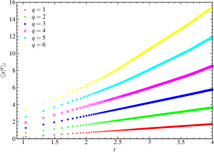
Since , we expect these moments to have power law growth, possibly with e.g. logarithmic corrections. We thus define the growth rates by [AHO03]
| (5.2) |
Corrections to power law growth are ignored by this definition. Numerically we calculate by fitting a straight line to a – plot of the th moment in the long-time regime. The growth rates are shown in Fig. 5.6 for the polygonal Lorentz channel in the normal diffusion case. We see a qualitative change at around between two approximately linear regimes. Results of this type have been reported in a variety of models in [CMMGV99, FMY01, AC04] and are sometimes referred to as ‘phase transitions’. Physically this corresponds to a change in importance between ballistic trajectories and diffusive trajectories [FMY01].
We also remark that it was proved in [AHO03] that is a convex function of , assuming that the limit defining exists. This considerably restricts the possible behaviour. Again the data points on the graph violate this and so cannot be correct; nonetheless we believe that the data gives an impression of the true behaviour. In particular, the numerical accuracy of the high-order moments is not good, since they become very large: the rate of increase in the high-order regime cannot in fact exceed , contradicting the best-fit line333 [Higher moments are dominated by extreme values, which must be eliminated to obtain reproducible results [SL06].] .
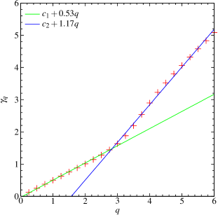
5.3.2 Velocity autocorrelation function
The above results provide some evidence of normal diffusion: we have , so that the growth of the variance of the position distribution (and hence of the mean squared displacement) is asymptotically linear. We can attempt to confirm this by studying the velocity autocorrelation function , which must be integrable for the diffusion coefficient to exist. As seen in Fig. 5.7, this is an oscillatory function whose maxima seem to decay approximately as . (Statistical errors (not shown) dominate for large time.) Since there is also cancellation due to the oscillation, this gives weak evidence that the velocity autocorrelation function is integrable.
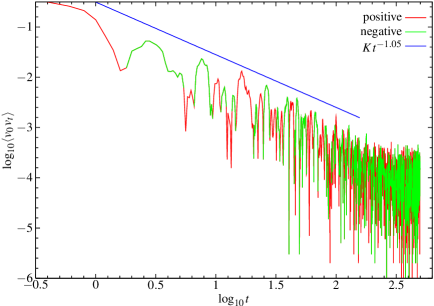
It was suggested in [LM93] to consider instead the integrated velocity autocorrelation function
| (5.3) |
since the delicate cancellations in will be seen more robustly in . If is integrable then as . If decays as, for example, then diverges logarithmically, so that plotting against should give a linear asymptotic growth. Figure 5.8 provides some evidence that is integrable, since an asymptotic limit seems to be attained as increases. Thus overall we have good evidence that the mean squared displacement can grow asymptotically linearly, although we have not ruled out a small logarithmic correction444 [This point is again addressed in [SL06].] .
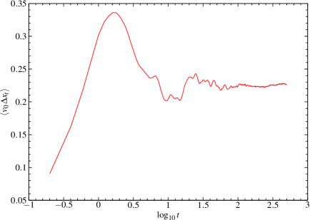
5.3.3 Fine structure
The shape of the displacement density was considered in [ARdV02] using histograms, but the results were not conclusive. Here we use the more refined methods developed in Chap. 4 to describe the fine structure and to show that the position and displacement distributions do seem to be asymptotically normal.
Figure 5.9 shows the position density in the Alonso model at a particular time. Following the method of Sec. 4.4, we can calculate the fine structure function as the normalized height of available space at position . Taking the origin in the centre of the unit cell in Fig. 5.1, we have
| (5.4) |
for , with being an even function and having period , and . (The factor of makes a density per unit length.) This fine structure function is shown in the inset of Fig. 5.9. We demodulate by dividing by to give , which is also shown in the figure. We see that it is close to the Gaussian with variance .
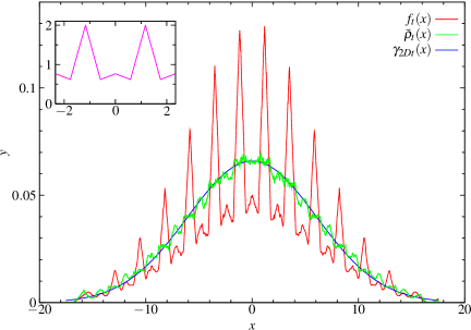
With the same notation as in Sec. 4.5.1, we can also calculate the fine structure function of the displacement density for the polygonal channel. The Fourier coefficients are and
| (5.5) |
for , where for we have
| (5.6) |
For the polygonal Lorentz channel, we have for that
| (5.7) |
where
| (5.8) |
This gives
| (5.9) |
In both cases we have and hence , so that is at least , whereas is Lipschitz continuous (i.e. Hölder with exponent ).
5.3.4 Central limit theorem
As for the Lorentz gas, we rescale the densities and distribution functions by to study the convergence to a possible limiting distribution. Again we find oscillation on a finer and finer scale and weak convergence to a normal distribution: see Fig. 5.10. Figure 5.11 shows the time evolution of the demodulated densities . There is an unexpected peak in the densities near for small times, indicating some kind of trapping effect; this appears to relax in the long time limit to a Gaussian density. Again we conjecture that we have uniform convergence of these demodulated densities to a Gaussian density.
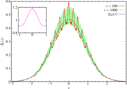
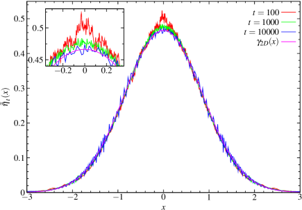
Figure 5.12 shows the distance of the rescaled distribution functions from the limiting normal distribution, analogously to Fig. 4.13, for several values of for which the mean squared displacement is asymptotically linear. The straight line fitted to the graph for has slope , so that the rate of convergence for this polygonal model is substantially slower than that for the Lorentz gas, presumably due to the much slower rate of mixing in this system. A similar rate of decay is found for , while and appear to have a slower decay rate. Nonetheless, the distance does appear to converge to for all these values of , providing evidence that the distributions are indeed asymptotically normal, i.e. that the central limit theorem is indeed satisfied. A similar calculation for the polygonal Lorentz channel (for the parameters used above) gives a convergence rate of , of the same magnitude as for the Alonso model.
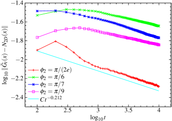
5.4 Anomalous diffusion
In dispersing Lorentz gases, there is a weak form of anomalous diffusion, with the mean squared displacement growing as for large : see Chap. 6. In polygonal billiards of many types, however, a strong type of anomalous diffusion has been observed, with for some . Note that the maximum possible rate is , since due to the finite particle speed.
As stated above, we find anomalous diffusion in our models precisely when there are parallel scatterers in the unit cell. Previous observations of anomalous diffusion in billiard models include [ZE97, Zas02, LWH02], and [PZ01] in discrete time, but they do not seem to have explicitly related the occurrence of anomalous diffusion to the geometry of the system. We remark that in [Zwa83] a model was presented for which the unit cell is a rectangle with a small window in one edge. It was stated that the growth exponent of the mean squared displacement depends on the number-theoretic properties of the aspect ratio of the rectangle. It would be interesting to revisit this model in the light of our results.
5.4.1 Moments
Figure 5.13 shows a typical plot of the mean squared displacement when . The long-time behaviour is well described by
| (5.10) |
where .
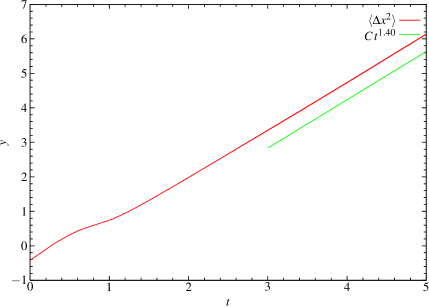
Figure 5.14 shows the growth exponent of the higher order moments for the polygonal Lorentz channel. There are two different linear regimes, as previously, with a crossover occurring near . Figure 5.15 shows the same for the zigzag model, for which there does not seem to be a crossover, and we have strong anomalous diffusion under the definition of [CMMGV99], where for all , with the constant given by for these parameters.
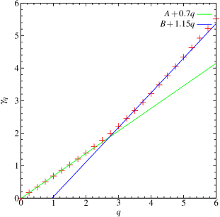
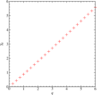
5.4.2 1D densities
Since the mean squared displacement grows like with , the scaling used in the central limit theorem cannot give densities which converge in any sense, since the variance of the rescaled densities would still tend to infinity. Instead we rescale to keep the variance bounded, setting
| (5.11) |
This scaling was previously used in [PZ01] for the Poincaré map of an anomalously diffusive billiard.
Figure 5.16 shows the -position density. The fine structure is again mostly removed by demodulating by the fine structure function found above, although this demodulation does not seem to be as effective as previously; this could be an artifact of an insufficiently precise estimation of the original density, or it could reflect weaker mixing properties of the system.
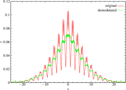
Figure 5.17 shows a sequence of demodulated densities rescaled as above. They appear to converge at long times to a limiting shape which is non-Gaussian. They are compared to a Gaussian with variance , where is the generalisation of the diffusion coefficient given by . The demodulated densities are, however, rather noisy; those for the displacement distribution are even more so.
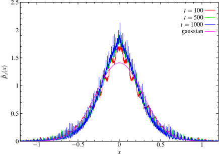
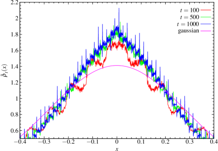
Zigzag model
Rescaled densities for the zigzag model are shown in Fig. 5.18; for long time we again have convergence to a limiting distribution. The spikes in the tails seem to correspond to long-lived propagating orbits. Note that there is no fine structure to take into account for the zigzag channel, since the channel width is a constant within the unit cell. The peak at has been observed previously in anomalous diffusion: see e.g. [FMY01].
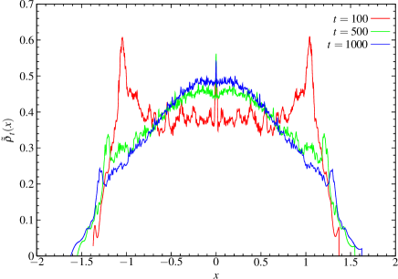
We remark that the unit cell of the zigzag model when the top and bottom scatterers are parallel can be reduced to a parallelogram with irrational angles. The mixing properties of the billiard flow inside such a geometry are not obvious, although we have checked that velocity autocorrelations decay as a power law. There may be an effect of slow ergodicity, where the system takes a long time to explore certain regions of phase space: see e.g. [KH98, PZ01].
5.4.3 Maxwellian velocity distribution
Just as for the Lorentz gas, we can consider the effect of a different distribution of velocities; this has been considered for heat conduction [LCW03, ARdV02].
Recall from Sec. 4.7 that if there is a speed distribution , then the mean squared displacement at time in 2D is given by
| (5.12) |
If a billiard system shows anomalous diffusion for particles with unit speed which looks like
| (5.13) |
then
| (5.14) |
Thus
| (5.15) |
Hence there is now a correction factor of the th moment of the speed distribution which enters, although the rate of growth is still . We have observed such a correction numerically.
5.5 Continuous-time random walk model for anomalous diffusion
A widely-used framework for understanding anomalous diffusion processes is the theory of continuous-time random walks (CTRW): see e.g. [Wei94, KBS87, ZK93]. This is a generalisation of standard discrete-time random walks where individual steps are still independent, but are now described by a density function , where is the probability of having a step with distance in which takes time in .
To be able to model super-diffusion, must have a coupled form [ZK93], such as
| (5.16) |
This form (called the velocity model in [ZK93]) models motion at a constant velocity for a time in the direction ; after each stretch the direction is randomised and a new step is taken. It gives the following long-time growth of the mean squared displacement :
| (5.17) |
when ; see [Gei95, KZS95] for reviews. More generally we have
| (5.18) |
where is the conditional probability of a step of length if we know that it lasts for time : see e.g. [Wei94, Sec. 2.5] and [SK89]. In general the rate of growth of the mean squared displacement will then also depend on the properties of .
Figure 5.19 shows a representative trajectory in the zigzag model with anomalous diffusion. From the figure we can see the importance of laminar motion, i.e. coherent motion in one direction along the channel. Referring to the above CTRW picture, we try to model the motion using random walks where the steps are stretches of laminar motion.


We define laminar motion in the zigzag model as follows. For each section (half a unit cell) of the channel, we assign a vector parallel to the channel walls, with a consistent -direction along the channel. We say that two consecutive stretches of trajectory (between bounces) are part of the same laminar motion if they have the same directions along the channel, as measured by . Figure 5.20 shows a scatterplot representing the joint distribution of periods of laminar motion with -displacement along the channel and taking time . Part (b) of that figure shows that allowed values of are restricted to being near integers, since a laminar motion cannot end in the middle of a unit cell. (A similar effect in infinite horizon 2D periodic Lorentz gases was described in [Ble92], although no figure was given.) We can thus regard the walk as taking place on a one-dimensional lattice.
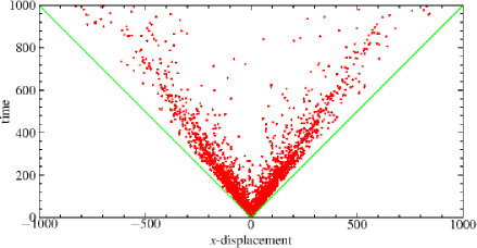
We see that the distribution is non-trivial, and the figure does not give much hope of finding an analytical expression for it. However we could hope that an approximation of the form referred to above may be adequate, for some speed , since the distribution is somewhat concentrated along diagonal lines. Figure 5.21 shows the tail region of the density and its distribution function. If we assume the velocity model form, then the observed long-time power law decay , shown in Fig. 5.21, gives and hence a mean squared displacement . This compares with the observed growth . The agreement leaves room for improvement, showing that we must use a more general CTRW model incorporating information on the complete , or perhaps reject any CTRW model which omits important information on correlations between consecutive laminar trajectories; such correlations can be seen in Fig. 5.19, for example.
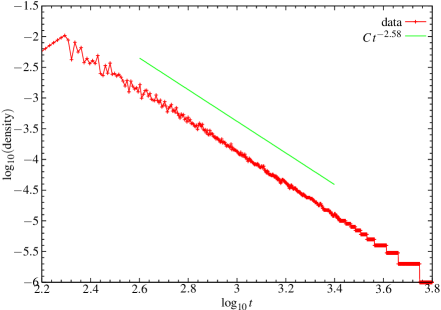
Figure 5.22 shows a trajectory in the polygonal Lorentz gas model. Despite the fact that anomalous diffusion is also found in this model when there are parallel scatterers, the mechanism is much less clear, since it does not seem possible to identify an obvious candidate ‘laminar motion’ in this model by looking at sample trajectories.

5.6 Crossover from normal to anomalous diffusion
Since anomalous diffusion occurs under certain geometrical conditions, whereas normal diffusion seems to be more general, it is of interest to ask how the crossover from one to the other occurs when the geometry is changed to approach one where anomalous diffusion occurs. We study the two models introduced above to show numerically how the crossover occurs.
In the following we fix all geometrical parameters except for , which we vary according to . Anomalous diffusion is found for , with asymptotically normal diffusion found for any . It is thus of interest to study how the statistical behaviour changes from one asymptotic regime to the other as the symmetrical configuration is approached when .
Figure 5.23 shows the mean squared displacement as a function of time for several values of . The same data is plotted on log–log axes in Fig. 5.24(a) and as deviations from a linear fit to one of the curves in Fig. 5.24(b). We see that as , the curves follow the anomalous diffusion curve (with slope ) for longer times, before a crossover occurs to asymptotic linear behaviour.
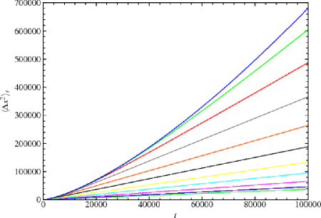

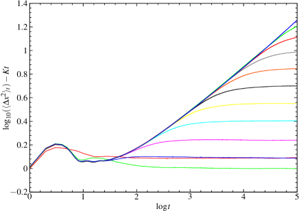
The intercept of the asymptotic linear growth for is related to the diffusion coefficient . As , the intercept moves up, corresponding to an increase in . Figure 5.25 shows the diffusion coefficient in this asymptotic linear regime as a function of , obtained via the slope of the mean squared displacement. Note that it is clear from Fig. 5.24 that the asymptotic linear growth regime has not yet been reached for the smallest values of , so that the diffusion coefficients for those values are expected to be underestimates.
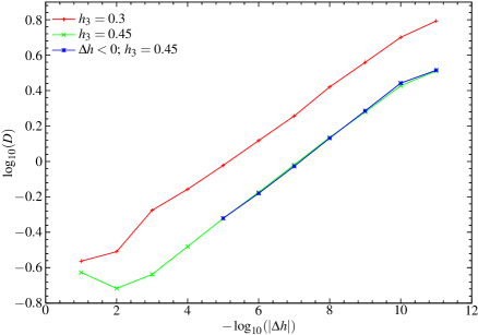
We obtain a straight line on a log–log plot, and a fit in the region gives
| (5.19) |
The diffusion coefficients obtained for negative values of are also shown for , and it is clear that the growth rate is the same. We hence obtain the power law behaviour
| (5.20) |
Note that this agrees with when .
We could also consider the crossover time, i.e. the time required to switch from the anomalous diffusion regime to the linear growth regime. One possible definition of this time could be as the intersection of two straight line fits: a fit to the initial anomalous growth and a fit to the asymptotic normal growth. A construction of this type was used e.g. in [CGvB04] in a different context. From Fig. 5.24 we see that this crossover time tends to as , and we could study555 [This was done in [SL06], where a simple scaling form was found allowing a data collapse of the data for different .] the dependence of this time on .
5.6.1 Zigzag model
There is a similar crossover to anomalous diffusion when in the zigzag model; the growth of the moments is very similar to the polygonal Lorentz channel. Figure 5.26 shows the growth of the diffusion coefficients as . A fit gives
| (5.21) |
and hence
| (5.22) |
so that we again obtain a power law, but with a different rate of growth than in the polygonal Lorentz model.
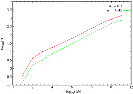
5.6.2 Qualitative explanation
In the zigzag model we can find a qualitative explanation of the above observations as follows. If we start a trajectory with the same initial conditions in the cases and small, the latter trajectory will shadow (follow approximately) the former for a certain length of time. However, the latter will gradually (linearly in time) deviate from the first trajectory due to the (weak) defocusing effect of the boundaries, eventually becoming effectively decorrelated. For smaller values of , the shadowing will persist for a longer period.
We refer again to the CTRW model described in Sec. 5.5. For , we find that the density function is oscillatory, so that it is difficult to determine its decay rate; instead, Fig. 5.27 shows for long times, where
| (5.23) |
It decays like , so that , giving , which according to (5.17) gives normal diffusion, as required. However, we may not have managed to attain the asymptotic regime in this calculation. For smaller we expect the distribution to have a progressively longer tail, so that the average laminar length will be longer, resulting in a larger diffusion coefficient as seen in the numerical experiments.
Again we remark that although the same behaviour is found in the polygonal Lorentz model at the level of the statistical properties, it is less clear how to obtain a qualitative understanding in that case without identifying the type of laminar behaviour which is presumably responsible.
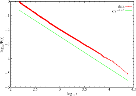
Chapter 6 Three-dimensional periodic Lorentz gases
We would like to extend the detailed knowledge available for 2D systems to study more physically relevant 3D periodic Lorentz gases. Relatively little work has been done on higher-dimensional models, since computation time increases and technical difficulties arise, some of which are discussed below. In this chapter we succeed in addressing some of these issues and point out where more work is still required111 [Some results from this chapter are included in a submitted manuscript [San], which also contains updated references.] .
Previous work on 3D periodic Lorentz gases in a physical context includes that of Bouchaud & Le Doussal [BLD85], who studied the Lyapunov exponent and the decay of velocity autocorrelation functions for simple (hyper-)cubic lattices in dimensions, and Dettmann et al. [DMR95], who studied a 3D hexagonal close-packed lattice with an electric field and a thermostat (a device for keeping the kinetic energy of a particle constant, despite the energy input due to the electric field), showing that the Lyapunov exponents satisfied a conjugate pairing rule. Rigorous results, discussed in more detail below, are proved in [Che94] and [GW00].
We first review results which show that higher-dimensional Lorentz gases with finite horizon exist. We then construct a particular 3D model with overlapping scatterers which has a finite horizon regime, analogously to the model studied in Chap. 3; in this regime we show numerically that our model is diffusive. We then consider the effect on the statistical properties of allowing an infinite horizon, and find that there are two qualitatively different types of infinite horizon regime.
6.1 Existence of higher-dimensional Lorentz gases with finite horizon
Chernov [Che94] extended the results of [BS81, BSC91] to higher-dimensional () periodic Lorentz gases. He proved222Some details of the proofs in [Che94] are corrected in [BCST02, BCST03]. fast (at least stretched exponential) decay of correlations for the billiard map, and the central limit theorem and functional central limit theorem for Hölder continuous observables for the billiard flow, when the scatterers are disjoint and have sufficiently smooth () boundaries, and the finite horizon condition is satisfied333Recall from Sec. 3.1 that a periodic Lorentz gas satisfies the finite horizon condition if no trajectory can be extended arbitrarily far without hitting a scatterer.. However, no explicit example of a model satisfying the assumptions was given in [Che94], even in the 3D case. In fact we are not aware of any examples of such models in the literature; unfortunately we have also been unable to construct an explicit example.
6.1.1 Rigorous results from convex geometry
Several results in convex geometry, which are seemingly unknown in the physics community, bear light on the possibility of constructing higher-dimensional periodic Lorentz gases with finite horizon.
In [Hep61] it was shown that any lattice packing of spheres in 3D has an infinite horizon, and in fact a cylindrical hole, the three-dimensional version of the corridors in infinite horizon 2D periodic Lorentz gases. Such a hole consists, in billiard language, of a collection of parallel trajectories (forming a cylinder), none of which ever collides with a scatterer.
We remark that the term ‘lattice’ in this result refers to a set of points of the form , where ; thus geometers’ lattices are what physicists call Bravais lattices [AM76]. For example, the hexagonal close-packed structure is not a lattice in this sense, although the face-centred cubic is. A ‘sphere packing’ is (roughly) a collection of touching, but non-overlapping, spheres.
The result was later extended to show the existence of cylindrical holes in lattice sphere packings of any dimension: see references in [HZ00]. This implies that to obtain a finite horizon it is necessary to have more than one sphere per unit cell; this was stated without proof in [CD00].
Recently it was proved in [HZ00] that this is no longer true if we consider arbitrary periodic structures, rather than just lattices, consisting of identical convex bodies. They showed that in any dimension there exist periodic arrays of non-touching spheres with finite horizon (although they did not use this terminology), and in fact with spheres replaced by any convex body. The proof is constructive, but it is not easy to convert it into the construction of an explicit example444M. Henk, private communication., since it involves finding sets of minimal cardinality satisfying certain properties.
This result implies that the class of models considered in [Che94] is indeed non-empty. We remark that in any such finite horizon model, the minimum number of spheres which can be seen from a given sphere has been shown to be at least : for references on this and related results see the review [Zon02, Sec. 5–6]. Hence any such structure must be quite complicated.
6.1.2 Attempts to construct a finite-horizon model
A common construction in solid state physics is to build lattices as stacks of layers, with each layer being a 2D triangular lattice of spheres (corresponding to the standard triangular 2D periodic Lorentz gas). Consecutive layers are placed in one of three possible positions, labelled , and , relative to the previous two layers [AM76]: a hexagonal close-packed structure corresponds to the choice , and the face-centred cubic to ; neither of these (somewhat surprisingly) has a finite horizon. (The face-centred cubic structure is a Bravais lattice, and so is covered by the theorem cited above, but the hexagonal close-packed structure is not.) We could ask if it is possible to produce a finite horizon by some other periodic ordering of s, s and s. However, in fact placing adjacent layers on top of each other creates cylindrical holes between the layers, so that there is always an infinite horizon. If we also require disjoint (non-touching) scatterers, then we would need to separate the scatterers slightly from their touching positions, thereby introducing more holes.
As an example, Fig. 6.1 shows the case of the face-centred cubic lattice: Fig. 6.1(a) shows the structure as built up from stacks of hexagonal close-packed layers, whilst Fig. 6.1(b) shows a cylindrical hole through the structure, as required by Heppes’ theorem quoted above. In fact this hole lies between two adjacent hexagonal layers, so that any structure built up of such layers would contain a similar cylindrical hole.
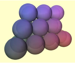
Another possibility for constructing explicit 3D models with finite horizon would be to make periodic layers with a lower density of spheres, but still with finite horizon within the layers. If the density were low enough, the next layer could be pushed down far enough to block the corridors between the layers and possibly obtain a finite horizon. However, we have not managed to construct a model in this way. We could also try constructing a model with, for example, ellipsoids instead of spheres, but again we have had no success.
6.2 Construction of 3D periodic Lorentz gas with overlapping scatterers
Here we present a 3D periodic Lorentz gas model analogous to the 2D model555In fact, we were led to the 2D model as a cross-section of the 3D model. of Chap. 3, which has a finite horizon in certain regions of parameter space. To accomplish this, however, we allow the spheres to overlap, which appears to be the only way of achieving a finite horizon with a simple model, as discussed above.
Allowing the spheres to overlap is at first sight non-physical; however, suppose that the moving particles are spheres of non-zero radius . In this case, the dynamics is the same as that of point particles moving through the same lattice, but with the radius of the scatterers increased by ; this radius could represent the effective radius of a particle interacting with the crystal lattice via a more realistic potential. This is the same construction originally used by Sinai [Sin70] to reduce two discs moving on a torus to a periodic Lorentz gas; see also the discussion in Chap. 1. We will find conditions under which the overlapping model can be regarded as a physical model in this way.
Note that allowing overlapping scatterers violates one of the key requirements in Chernov’s proof that the multi-dimensional Lorentz gas is diffusive [Che94]. Nonetheless, we expect physically that the system still possesses strong ergodic and statistical properties, and in particular is still diffusive. This seems to be corroborated by numerical experiments, as discussed below.
6.2.1 Construction of finite horizon model by blocking corridors
We consider a cubic unit cell of a 3D simple cubic lattice of spheres of radius . If the spheres do not touch, then there are lots of holes in the structure. In order to construct a finite horizon model, we need to block all of these holes. We first allow the spheres to overlap. The configuration in a plane through the centres of neighbouring -spheres then looks like Fig. 6.2. There is no longer an infinite horizon within this plane, and we have one corridor perpendicular to the plane.
We now add a new scatterer, with (different) radius , at the centre of the -unit cell. If we make the -sphere sufficiently large that its projection onto one of the faces of the unit cell blocks the hole in that face (Fig. 6.2), then we have blocked all corridors perpendicular to the faces.
6.2.2 Phase diagram
The construction of the phase diagram follows that of the 2D case: again we look for lines in parameter space across which the geometry of the unit cell undergoes qualitative changes. However, the additional freedom in dimensions makes the calculation more difficult.
Overlap of -spheres
The overlaps of the -spheres change as follows when we vary .
-
•
The -spheres overlap if and only if ; this is a necessary condition for a finite horizon in our class of models.
-
•
The space between the -discs on a unit face closes when two discs at opposite ends of a diagonal of the square touch, which occurs when ; for larger values of it is impossible for a particle to move between different unit cells, so the trajectory is localised and the diffusion coefficient vanishes.
-
•
The -spheres cover the entire unit cell when two spheres at diametrically opposite vertices of the unit cube touch, which occurs when , i.e. at .
Blocking vertical trajectories
Let be the minimal value of the radius of the additional scatterer required to block the vertical corridor (i.e. such that its vertical projection covers the space on a face between the -sphere overlaps, as in Fig. 6.2), and let be the width of the overlap of two -discs on a face; this is also the radius of the disc of intersection of two neighbouring -spheres with the mid-plane between them. The geometry is shown in figure 6.2.
We have and , so that and a necessary condition for finite horizon is
| (6.1) |


Blocking diagonal trajectories
We now must now block any diagonal corridors (diagonal relative to the lattice viewed as cubic cells). By symmetry, it suffices to block trajectories in the mid-plane of the unit cell: there is ‘most space’ in this plane. (Compare this to blocking diagonal angles at in 2D.)
The mid-plane is shown in Fig. 6.2; its geometry is the same as that of the 2D model considered in Chap. 3, after replacing by . If , then horizontal and vertical trajectories within this plane are already blocked, by definition of . Diagonal trajectories at will be blocked if either , which reduces to , or if .
If neither of these conditions holds, then, by continuity, there is an interval of non-zero size around the height of the midplane such that planes at heights lying in that interval also have an infinite horizon along trajectories at , so that there is a cylindrical hole of non-zero volume lying along this diagonal, and hence the structure has an infinite horizon.
Conditions for localised trajectories
If the or spheres are too large then they will overlap to such an extent that trajectories will be localised, as in the S and D regimes of the 2D model (Sec. 3.1.4).
Consider again the midplane shown in Fig. 6.2. Suppose that the - and -discs do not touch. Then any point outside the discs in the midplane is accessible from any other. In fact, since there are identical planes perpendicular to each of the coordinate directions, there is a connected network of empty space lying around the grid of lines parallel to the coordinate directions which join the centres of the -spheres. Hence for we do not have localised trajectories. We now show that in fact this is a necessary condition: all trajectories are localised if .
Consider cutting the unit cell by a horizontal plane which begins at the mid-plane and moves upwards. Let be the height of the plane above the mid-plane, and let the radius at height of the - and -cross-sections be and , respectively. Then , , and .
Trajectories will be localised if and only if there is a plane at some height in which there is no available space, i.e. for which the - and -discs fill this plane, for then there are barriers in each direction blocking escape, whilst if there is space in each plane then in fact this space must be connected all the way from to . From Sec. 3.1.4, we know that this blocking occurs exactly when
| (6.2) |
since the geometry in this plane is the same as the 2D geometry with and replaced by and , respectively. Considering when there exists an for which is equivalent to the following slightly different approach.
Taking coordinates with the origin at the centre of the unit cell (and hence at the centre of the -sphere), if the intersection point of the overlap of neighbouring -spheres with the -sphere is at then we have by symmetry and thus
| (6.3) | |||
| (6.4) |
since the intersection point lies on each sphere.
Expanding (6.4) and using (6.3) gives , and substituting into (6.3) then gives
| (6.5) |
so that an intersection exists if and only if , which is equivalent to , since .
We have , so that , and hence . Thus the condition for existence of the intersection is , i.e. . Equality occurs when , so that there is an intersection if and only if
| (6.6) |
The leftmost term is equal to ; the rightmost term is greater than , so that it is never attained for non-localised trajectories for which we must have . Hence the condition for intersection is that the - and -discs touch in the mid-plane, as claimed.
Condition for all space to be covered
To establish when the -sphere covers all the space left by the -spheres, consider first the case when , so that the -spheres leave holes on and near the unit cell faces. These holes will be covered by the -sphere once it is big enough that its intersection with the unit cell face covers the space on that face, i.e. if
| (6.7) |
which reduces to
| (6.8) |
or finally
| (6.9) |
When , we need to be large enough for the -sphere to cover the -hole inside the overlap of the -spheres. For this we need that the -disc covers the -hole between the -discs in the mid-plane. The geometry is exactly as in the 2D case, with replaced by , so we can quote the result:
| (6.10) |
Overlapping conditions
Note that if then the -spheres meet the -spheres, whilst if then neighbouring -spheres meet each other.
Phase diagram
The parameter space of the 3D model is shown in Fig. 6.3 for . The regimes are named as far as possible to agree with those of the 2D model in Sec. 3.1.4: if the name is the same as one for the 2D model, then the geometrical features and statistical properties are similar. The diagonal from top left to bottom right is the boundary line separating regimes where the -spheres do not touch the -spheres (below) from those where the - and -spheres overlap (above). This cuts several of the other regimes.
Several regimes do not occur in the 2D model. N has localised motion in cells centred on the -spheres, but with the -spheres overlapping the -spheres. In IH4 the -spheres meet each other and also the -spheres but still with infinite horizon. In IH0 nothing is touching and we have a strongly infinite horizon (see also Sec. 6.5).
Note that the finite horizon (FH) regime consists of two disjoint pieces, corresponding to the two different ways of preventing diagonal infinite horizon trajectories detailed above. In fact, the top of FH2, above the line , could be regarded as a third finite horizon regime. Here, the -spheres meet each other (as well as the -spheres), so that there is a single connected scatterer network with an interconnected hole inside it.
Figure 6.4 shows the model in the finite horizon regime with the - and -spheres not overlapping. We can check by rotating the model that it does indeed have finite horizon, since no holes can be seen in the complete unit cell.
6.2.3 Physical realisation with a moving particle of non-zero size
The overlapping system with radii and studied above can be regarded as physical if it is a reduction of a system with a moving sphere of radius travelling within a lattice of spheres with radii and with no overlaps. Regarding and as position vectors in the phase diagram determined above, the reduction condition is
| (6.11) |
which corresponds geometrically to translating by the vector from the initial point on the phase diagram. The system will be diffusive if this lands in the FH regime.
For the initial point to correspond to a system where no spheres overlap, we must start in the region IH0. In fact, any point in IH0 corresponds to some point in FH via a translation by some vector , except for a line at passing through the point where the FH1 and FH2 regions touch.
6.3 Normal diffusion in the finite horizon regime
We now use techniques developed in previous chapters to give strong evidence that we have normal diffusion in the finite horizon regime. We emphasise that the arguments of [Che94] require disjoint scatterers, and so do not immediately apply to our model; nonetheless we expect that those methods should be able to be refined to deal with our case and prove normal diffusion, even in the strongest sense that the functional central limit theorem is satisfied.
6.3.1 Decay of velocity autocorrelations
From the discussion of the Green–Kubo relation in continuous time of Sec. 2.3.8, a necessary condition for the existence of the diffusion coefficient (which is the weakest type of normal diffusion) is the integrability of the velocity autocorrelation function . Since this function is highly oscillatory and rapidly becomes small, it is difficult to study. It was thus suggested in [LM93] to look instead at the integrated velocity autocorrelation function , given by
| (6.12) |
The integration in the definition of acts as a smoothing operation which deals efficiently with the highly oscillatory nature of . Note that in this definition we do not need to perform a direct numerical integration of the function ; such an approach was taken, for example, in [MM97].
If is integrable, then as , where is the spatial dimension and is the diffusion coefficient. We find numerically that decays so fast that we cannot extract any information about it, and we do not plot it. Similarly reaches very rapidly a limiting value, which it then oscillates around in a random fashion. This provides evidence that is integrable and hence that exists, giving normal diffusion.
6.3.2 Growth of moments
Figure 6.5 shows the growth rates of the moments as a function of . As in the 2D finite horizon case (not shown), they satisfy , so that we have a strong form of normal diffusion; we conjecture that the functional central limit theorem is satisfied for our model in the finite horizon regime, as was proved in [Che94] in the case of disjoint scatterers.
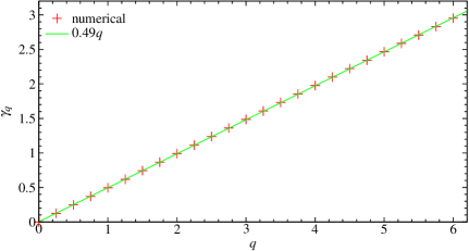
6.3.3 Shape of distributions and central limit theorem
Knowing that the mean squared displacement grows asymptotically linearly in the finite horizon regime, we can apply the techniques of Chap. 4 to investigate the shape of densities and the central limit theorem.
Restricting attention to 1D projections of the position distribution, we need to calculate the analogue for our model in the finite horizon regime of the available height function used in Chap. 4. This analogue is the available area, which we denote by , in a cross-section perpendicular to the -axis at distance from the centre of the -sphere; we refer to this cross-section plane as the -plane. We denote the radii of the cross-sections of the - and -spheres in that plane by and , respectively, where we again use the convention that when .
Figure 6.2 can be thought of as depicting a generic cross-section, after possibly adding a small -cross-section in the centre. Denote by the area of each overlap of -discs in the -plane. Then
| (6.13) |
where if then
| (6.14) |
whilst there is no overlap if . Here
| (6.15) |
is the anti-derivative of (with respect to ). Further, is the volume of the available space in a unit cell given by
| (6.16) |
where
| (6.17) |
is the volume of the intersection of two neighbouring spheres. (Similar overlap calculations were used in [San00] in a related context.) In the above calculations we have for simplicity restricted the calculation to the case where the - and -spheres do not overlap.
The inset of Fig. 6.6 shows the available space function as calculated above, whilst the main part of that figure shows the 1D position density and the demodulated version , for certain geometrical parameters in the finite horizon regime which we believe to be representative. Again we see that the demodulated density is very close to Gaussian, and we have confirmed numerically that the central limit theorem holds with rate of convergence , close to the optimal as discussed in Sec. 4.6: see Fig. 6.7.
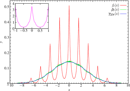
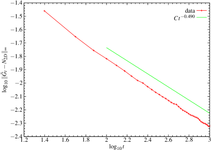
6.3.4 Geometry dependence of diffusion coefficients
Figure 6.8 shows the geometry dependence of the diffusion coefficient over the two finite horizon regimes. In FH1 the behaviour resembles that in the 2D case, although the angle at which the curves approach on the right hand side is different; in particular, here too there is a qualitative change in behaviour with a non-trivial maximum which disappears for larger values of .
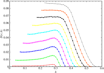
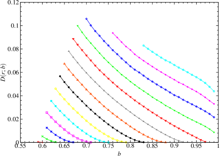
6.4 Statistical behaviour in the infinite horizon regime
6.4.1 Shape of 2D distributions
How can normal diffusion fail to hold in dispersing billiards with infinite horizon? Figure 6.9 shows scatterplots representing the position and displacement distributions for representative parameters in the infinite horizon regime of a 2D square Lorentz gas. These distributions have a distinctive shape caused by the possibility of particles travelling arbitrarily far without ever hitting a scatterer. Bleher [Ble92] showed, assuming some natural conjectures666 [A complete, rigorous proof has now been given [SV07].] , that the mean squared displacement in this case grows like as . He also showed that
| (6.18) |
where is a normal random variable; this is a central limit theorem type result with a different normalisation constant. The faster growth rate of the variance corresponds to the tails of the distribution visible in Fig. 6.9.
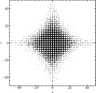
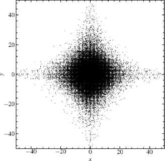
6.4.2 Discrete-time dynamics
Following [Ble92] (who discussed the 2D case), we write
| (6.19) |
where is the position at the th collision (occurring at time ) and is the free flight vector between the th and th collisions.
In the finite horizon regime the free path length is bounded above, so that is a piecewise Hölder continuous function defined on the collision phase space. The central limit theorem of [BS81, BSC91] can then be applied to show that converges in distribution to a normal distribution.
In the infinite horizon case, however, is no longer bounded and so cannot be piecewise Hölder continuous, since a continuous function on the compact phase space must be bounded. The central limit theorem thus does not apply. Defining the finite-time diffusion coefficient by
| (6.20) |
the limiting diffusion coefficient for the discrete time dynamics takes the form [Ble92]
| (6.21) |
if it exists.
In [Ble92] it was conjectured that (at least in 2D) decays fast for large , so that the infinite sum in (6.21) exists. However, it was proved there that , the second moment of the free path length for the billiard map, diverges (logarithmically), so that the first term in (6.21) is infinite and hence so are the discrete-time and continuous-time diffusion coefficients.
6.4.3 Obstructions to normal diffusion
Generalising the above to higher dimensions, there are two possible obstructions to normal diffusion outside the FH regime:
-
(i)
the continuous-time VACF decays slowly as a function of time , so that the Green–Kubo integral, giving as the infinite-time integral of this VACF, diverges; and
-
(ii)
the second moment of the (discrete-time) free path length diverges.
If neither of these obstructions is present, then we expect to have normal diffusion: this is certainly the case in the finite horizon regime treated above. We now discuss the situation in the infinite horizon regime, i.e. when there exist trajectories which never collide with the scatterers.
6.4.4 Review of two-dimensional case
Decay of velocity autocorrelations
The following type of argument seems to have first been published in [FM84]. Consider a 2D lattice with infinite horizon (for example a square lattice of scatterers of radius ). Due to the infinite horizon, there exist corridors in the structure, i.e. empty regions of constant, non-zero width, extending infinitely far in opposite directions. Bleher [Ble92] gives a detailed description of these corridors.
Consider one particular corridor, of width . Take coordinates such that the -axis is parallel to the centre-line of the corridor and the -axis is perpendicular to it, with the origin at an arbitrary point on one edge of the corridor. Let be the angle from the -axis.
We consider initial conditions in whose trajectories have no collisions within (continuous) time , and in fact remain inside the corridor at least until time ; thus these trajectories are straight during this period, so that . A trajectory emanating from in the direction from the -axis will not leave the corridor within time provided the line segment of length at angle ends within the corridor, i.e. provided , considering only one direction of flight down the corridor initially. The geometry gives
| (6.22) |
The Green–Kubo formula for the diffusion coefficient means that we are interested in the rate of decay of the velocity autocorrelation function (VACF) as . For large , is small, hence is small, so that .
For large enough , denoting the average of the VACF solely over those long trajectories which do not escape after time by , we thus have
| (6.23) |
Here, and are constants which are related to the area of intersection of the corridor with .
It is then argued in [FM84] that if the rest of the trajectories are more efficiently mixed, as we expect they are due to collisions with the scatterers, then the VACF averaged over those other trajectories will decay faster. Hence the rate of decay averaged over the whole of will be dominated by the slow decay of the long trajectories considered above. In this case, the integral of the VACF will diverge, so that the diffusion coefficient will not exist (or is infinite), implying that the system is super-diffusive.
Unfortunately the above argument is not rigorous, and indeed currently there are no rigorous results on decay of correlations for the billiard flow777 [Such results have now been obtained in the finite-horizon case [Che07].] , even in the finite-horizon case [CY00], although the recent results of [SV03] prove that , so that they show indirectly that must be non-integrable.
In [GG94] the exact result of Bleher for the rate of increase of the mean squared displacement was compared to numerical results. They pointed out, and we have confirmed, that the coefficient of the term is very small, so that it is difficult to observe numerically. Nonetheless it is sometimes possible to observe this effect by plotting against , as first suggested in the context of 1D maps in [GT84]. As argued in [GG94], if then the lower order terms presumably take the form
| (6.24) |
It then follows that
| (6.25) |
Introducting the variable , we then have
| (6.26) |
so that for large enough values of , i.e. for large enough values of , we should find asymptotically linear growth of .
Growth of higher-order moments
In [AHO03], a similar line of argument was used to give a lower bound on the rate of increase of higher order moments, as follows. A proportion of trajectories do not collide in time (as described above), so that for those trajectories we have the lower bound
| (6.27) |
where is the speed, so that .
They show that is a convex function of . We also know that and lie on the curve, that , assuming that the process acts at least as fast as a random walk, and that . These together lead to the conclusion that
| (6.28) |
Tail of free path distribution
As discussed in Sec. 6.4, the existence of is crucial for the possibility of having normal diffusion. We introduce the following functions:
| (6.29) | |||
| (6.30) |
(Recall that the billiard map preserves the measure on the phase space , and the billiard flow preserves the measure on the phase space .) These functions describe the tail of the distribution of the free path length considered in discrete time and continuous time, respectively. Note that in the discrete time case , where is the free flight vector.
In 2D, it was proved in [Ble92] that
| (6.31) |
By definition of expectation,
| (6.32) |
where the integral is a Lebesgue–Stieltjes integral. Integration by parts is valid for such integrals, so that
| (6.33) |
and hence the expectation diverges logarithmically.
The same result can be obtained using the following relation proved in [DDG97] (see also [Gol]):
| (6.34) |
for any function such that ; here denotes the derivative of . For we recover the known expression (see [Che97]) for the mean free path in terms of and discussed in Chap. 3, while for we obtain
| (6.35) |
Here we extend the definition of to the whole of as
| (6.36) |
the minimum time needed to collide with a scatterer.
Thus the second moment of with respect to exists if and only if the mean of with respect to exists. We now use an argument similar to those above involving the proportion of trajectories which have not collided within time : those trajectories have (continuous-time) free paths which are at least , so that integrating over initial conditions in one unit cell we have
| (6.37) |
The mean thus diverges logarithmically, and hence so does .
Summary
The above arguments all involve calculating the proportion of trajectories starting from a single unit cell which undergo no collisions up to time . For large these trajectories are ones which remain inside the corridor and lie on a circle of radius .
We obtain rigorous lower bounds for the higher-order moments as and for the size of the tail of the free path distribution function as , whilst we obtain only a heuristic estimate of as . In the next sections we shall apply these methods to our 3D Lorentz gas.
6.5 Simple cubic lattices
6.5.1 Free path distribution
We begin by discussing simple cubic lattices with and . In [Che94] it was stated that point (ii) of the previous section, i.e. divergence of holds in higher dimensions, and that the proof is “easy to verify”, but it was not stated which configurations this applies to. For simple cubic lattices a proof was given in [GW00]. In the next section we show that in certain other geometries the result is in fact no longer true, so that the existence or otherwise of normal diffusion reduces in that case to determining if (i) holds.
The method of [GW00] to prove this result is to generalise the method discussed in the previous section, by using the existence of free planes (called ‘sandwich layers’ in [GW00]) in the simple cubic lattice. These are infinite planes which do not intersect any scatterer, and are the 3D analogue of corridors related to infinite horizon trajectories (which we can think of as ‘free lines’) in 2D888 [Figures showing the different types of holes in 3D, as well as an analytical argument for systems of any dimension, are given in a submitted manuscript [San].] .
Analytical argument
Analogously to the calculations in the previous section, we need to find the proportion of trajectories remaining inside a sandwich layer and lying on a sphere of radius . The intersection of these two objects is approximately a circle with non-zero width, and the proportion is then the ratio of the area of this thickened circle, which is , divided by the area of the sphere of radius . The ratio is hence . A more careful argument, taking account of the intersections of such circles corresponding to different sandwich layers, shows that the same result holds [GW00]. We remark that this result was also stated in [FM84].
The argument of the previous section now gives a lower bound on the size of the tail of the free path distribution for the billiard flow of , so that again the expectation diverges.
Numerical calculation
Figure 6.10 shows the tail of the free path distribution for the billiard map, for two simple cubic lattices. This was obtained by recording only values of the free path exceeding a certain lower threshold, since otherwise the predominance of small values hides the information about the tail. A straight line corresponding to a decay rate of is also shown. Although the data appear to decay slightly faster than this, the decay rate is decreasing for large ; we believe that the asymptotic behaviour does obey the analytical prediction.
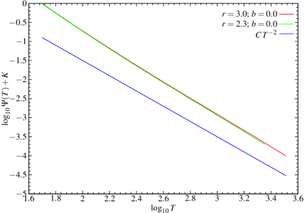
6.5.2 Higher-order moments
The growth rate of the higher-order moments is shown in Fig. 6.11. They are in good agreement with the analytical prediction, which in this case is the same as in the 2D case reviewed in the previous section:
| (6.38) |
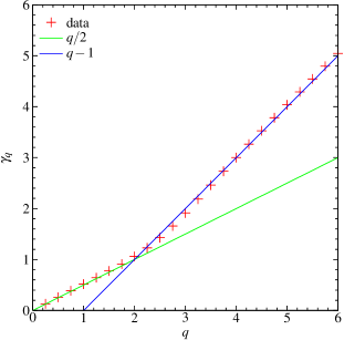
6.5.3 Decay of velocity autocorrelations
Figure 6.12 shows the velocity autocorrelation function (VACF) as a function of time . A fit to the less-noisy central part of the graph (also shown) gives a power law decay with an exponent which is close to . In Fig. 6.13 we also show , the integrated velocity autocorrelation function. If as , then we expect that
| (6.39) |
so that Fig. 6.13 plots as a function of . The linear growth for long time provides confirmation of the non-integrability of . We note that appears to converge to monotonically from above.
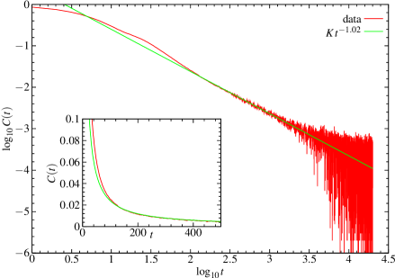
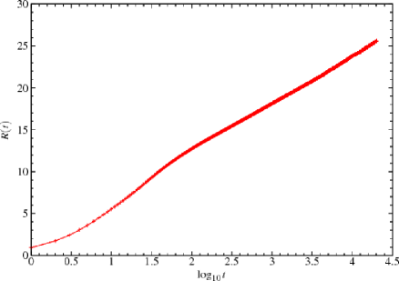
6.6 Lattices with cylindrical holes
6.6.1 Tail of free path distribution
Analytical argument
In the previous section we showed that the existence of free planes in the structure implies the divergence of , and hence the non-existence of the diffusion coefficient. However, for our model it is possible to block all free planes, either with the -spheres overlapping, or for large enough values of with the -spheres non-touching, leaving only holes of cylindrical type. The previous argument proving the divergence of now no longer holds, and in fact this quantity is finite, as follows.
Again we calculate the proportion of non-colliding trajectories of length , now which remain inside a cylindrical hole of radius . The set of these allowed directions along the cylinder is a circle of area (approximately) , independent of , whilst the set of all possible directions is the surface of a sphere of radius , with total area . (Actually there are two such circles in opposite directions along the cylinder.) The proportion of such trajectories is thus , compared to in two dimensions and in the case of simple cubic lattices.
This gives a decay rate of for the distribution function of the free path length for the billiard flow, so that exists and hence by (6.35) we also have . Thus point (ii) of Sec. 6.4 is no longer an obstruction to the possibility of normal diffusion. This does not appear to have been observed previously, although we later discovered that it was stated in [BGW98] (see also [GW00]) that there is a maximum decay rate of of in space dimensions. No details of the derivation were given, although presumably the argument was based on a similar idea. We however give explicit examples of models where this optimum value is attained.
Numerical results
[The numerical results in this section are incorrect. This is
due to the use of an incorrect method for generating the initial velocity
distribution. The initial velocities should be generated uniformly on a unit
sphere (since the speed is fixed to be ). The incorrect method used for the
numerical results depicted here was to distribute uniformly the spherical angles
and , and then assign the components of the velocity based on
these angles. This method, however, does not produce a uniform distribution
on the sphere, but rather produces a noticeable concentration of
directions close to the poles of the sphere. These concentrations align with
the holes in the structure, thus skewing the results sufficiently to make it
impossible to see the expected effect.
Correct numerical results are given in a submitted
manuscript [San].
There, the initial
velocities are correctly distributed uniformly on the sphere, by choosing
the velocity vector uniformly in , rejecting those with
, and then normalising to unit length. This generates
points uniformly on the unit sphere.
We find that diffusion is indeed normal, as the heuristic argument predicts, if
the only holes are cylindrical.
]
Figure 6.14 shows the tail of the free path distribution for the billiard map for two geometries for which the only holes are cylindrical. The tails decay as , so that , in agreement with the analytical calculation. We remark that the step-like character visible in Fig. 6.14 corresponds to the fact that the mass of the distribution is localised near points of a periodic lattice, as remarked for the 2D case in [Ble92]. We do not expect to see this effect in the continuous-time free path distribution, and indeed it is absent in plots of that distribution given in [GW00].
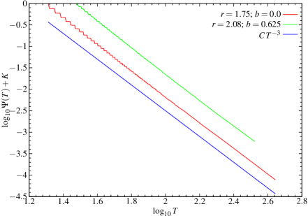
6.6.2 Higher-order moments
The generalisation to 3D of the argument of [AHO03] discussed above gives
| (6.40) |
This does not give enough information to determine uniquely the shape of the curve as it did in two dimensions, although it does show that it must grow like for large . Numerically we find that the data, shown in Fig. 6.15, fit well the function
| (6.41) |
The occurrence of the number here is perhaps related to the fact that we are now in space dimensions.
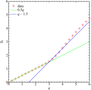
6.6.3 Velocity autocorrelation function
The decay of the velocity autocorrelation function at long times has a lower bound of , by the 3D version of the Friedman–Martin argument discussed above. It is thus now possible that the VACF is integrable and thus that the diffusion coefficient could exist, despite the infinite horizon.
Figures 6.16–6.18 show the growth of the integrated velocity autocorrelation function for several sets of geometrical parameters. As argued in the previous section, if as then we expect . The data in Fig. 6.16 provide strong evidence that for and , we do have such a decay, and hence that the diffusion coefficient does not exist in this case.
Figure 6.17 shows for and . This differs from the previous plot in the presence of a large central scatterer which severely restricts the size of the cylindrical holes. The figure is not conclusive, but it is possible to believe that converges as , implying that .
The most interesting case is that for , , shown in Fig. 6.18, since here the scatterers are disjoint. The data here seem to be consistent with , and hence , although perhaps the growth levels off for larger values of . We have also looked directly at , but again this converges rapidly to zero. There is some evidence that it oscillates around zero, which gives more chance of having convergence.
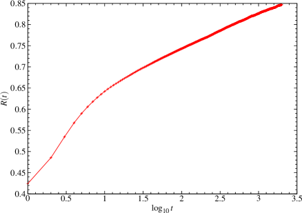
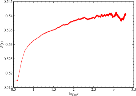
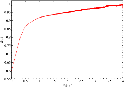
These remarks suggest that there may be a possibility of having normal diffusion, in the sense of asymptotically linear growth of the mean squared displacement, even in the presence of an infinite horizon, provided that there are only cylindrical holes; and this may even be possible with disjoint scatterers.
However, our numerical evidence also points to the fact that many parameters for which there are ‘large’ cylindrical holes in fact have , resulting in super-diffusion. (We remark that extending our numerical results to longer times would be difficult, since the calculations for Fig. 6.18 required a total of approximately 6 weeks of CPU time on modern workstations, distributed over 16 processors.) This slow decay is not predicted by the heuristic arguments given above, and it is important to determine its origin. One possibility could be that in fact there are strong correlations between flights along the cylindrical holes, so that the sum in (6.21) does not converge.
Chapter 7 Conclusions and future directions
7.1 Conclusions
We have studied geometrical, statistical and physical aspects of deterministic diffusion in three classes of billiard models.
We first discussed how best to estimate diffusion coefficients in billiard models from numerical data, presenting a method which estimates the width of the sampling distribution of the diffusion coefficient in terms of the rate of growth of the width of the distribution of the mean squared displacement.
We applied these numerical estimates in a 2D periodic Lorentz gas model to study the geometry-dependence of the diffusion coefficient, finding an unexpected qualitative change in behaviour as one of the parameters is varied. We extended a previously-known random-walk approximation to our model, showing that there are two regimes where it can be applied. We then considered a Green–Kubo formula, the zeroth-order term of which is this random-walk approximation. We showed how to improve the justification of the derivation of this formula. We also made preliminary investigations on the variation of the diffusion coefficient when the symmetry of the system is reduced.
In the same 2D periodic Lorentz gas model we then studied the shape of position and distribution functions, which we know converge to normal distributions at long times. Using a method which we believe is more appropriate than the usual histograms in this case, we showed that at finite time the densities possess a fine structure which prevents them from converging pointwise to Gaussians. We showed how this fine structure could be understood in terms of the geometry of the billiard domain, giving an analytical expression for the fine structure function for both position and displacement distributions.
Using these expressions, we showed that demodulating the densities by the fine structure gives functions which describe the two-dimensional density in a quasi-one-dimensional channel; information about these 2D density functions is otherwise difficult to obtain. This demodulation eliminates most of the very fine-scale oscillations, resulting in much smoother functions which seem to converge uniformly to Gaussian densities, strengthening the standard central limit theorem. Nonetheless, in certain parameter regimes these underlying densities themselves possess a type of fine structure, now corresponding to a nearly-uniform distribution within traps. We also used the knowledge of the fine structure to give a physical picture of the rate of convergence in the central limit theorem.
We considered the effect of imposing a non-constant distribution of particle speeds. We showed that for a general speed distribution with finite mean this does not affect the mean squared displacement. In the special case of a Gaussian distribution of velocities, however, we showed that the resulting limiting position distribution is skewed away from a Gaussian shape. Our analytical calculations of the resulting shape matched numerical results very well once the densities had been demodulated by the relevant fine structure function.
We studied the extent to which similar statistical properties hold in a polygonal billiard channel for which there are very few rigorous results. Although chaotic and mixing properties are much weaker for this model, we showed that similar methods can be applied, giving evidence that normal diffusion can occur, in the sense that the mean squared displacement can grow asymptotically linearly in time. We also confirmed that the central limit theorem can be satisfied, but with a slower rate of convergence than for the Lorentz gas. We established in several particular cases that the existence of parallel scatterers in the structure results in anomalous diffusion, and conjectured that this is generally the case. We found a crossover from normal to anomalous diffusion when this geometrical configuration is approached. We were able to understand this qualitatively in terms of a continuous-time random walk model, although we found that the quantitative prediction of a simple version of that formalism did not match numerical data well.
We finally discussed to what extent results on two-dimensional periodic Lorentz gases can be extended to the more physically realistic three-dimensional case. We constructed a 3D periodic Lorentz gas with overlapping scatterers and showed that it has a finite horizon regime, in which it exhibits normal diffusion. We discussed how different types of holes in the structure affect the statistical properties, giving evidence that it may be possible to have normal diffusion even when corridors exist, provided they are small enough.
7.2 Future directions
Our results point in several directions:
-
•
We hope that it is possible to find a better physical model of diffusion in the 2D Lorentz gas which can predict qualitative features of the geometry dependence of the diffusion coefficient.
- •
-
•
It may be possible to develop a more quantitative version of the qualitative arguments given in Sec. 5.4 to model anomalous diffusion in polygonal billiards. In particular it would be interesting to derive (approximations to) the step length distribution in the continuous-time random walk model for the zigzag model, directly from the shape of the unit cell.
-
•
Our analysis of the fine structure in Chap. 4 may have implications for the escape rate formalism for calculating transport coefficients (see e.g. [Gas98]), where the diffusion equation with absorbing boundary conditions is used as a phenomenological model of the escape process from a finite length piece of a Lorentz gas; analyzing the fine structure in this situation could provide information about the validity of the use of the diffusion equation in that context.
-
•
Further investigation is needed of the effect of cylindrical holes in 3D models described in Sec. 6.6. It is important to establish if (and to what extent) it is possible for a 3D periodic Lorentz gas with non-overlapping scatterers to have normal diffusion.
-
•
The arguments discussed in Sec. 6.6 relating to the possibility of faster decay of correlations and free path distributions should extend to billiards in higher dimensions; in particular, we should in principle be able to obtain bounds on the decay of correlations and the free path distribution of hard-sphere fluids, by treating them as billiards in a high-dimensional phase space, as described in Sec. 1.2.3. An understanding of the shape of ‘free’ regions in the configuration space, together with arguments similar to those of Sec. 6.6, should give bounds on and/or estimates of the rate of decay of velocity autocorrelations and of the free path distribution, corresponding to the trapping effects referred to in [CY00]. However, the complicated geometry of the high-dimensional phase space [Che97] means that this would be difficult to implement.
We expect that billiard models will remain of interest to mathematicians and to physicists in the future.
Appendix A Convergence of rescaled solutions of the diffusion equation to a Gaussian
We show that the rescaled solution of the diffusion equation starting from an initial density which decays sufficiently rapidly at infinity converges to a Gaussian shape as .
A.1 Pointwise convergence
Let be the solution of the diffusion equation with initial condition which is a density, i.e. which satisfies and . We also assume that is a piecewise continuous function and decays sufficiently fast at infinity. By translating the coordinate origin if necessary, we further assume that the centre of mass of the initial condition is fixed at the origin: .
Define the rescaled solution . Then
| (A.1) | ||||
| (A.2) |
For fixed , the argument of the exponential in the integrand in (A.2) tends to as . Hence the integrand tends to and it is bounded above provided decays sufficiently fast at infinity, for example if it is exponentially localised in the sense that
| (A.3) |
for some constant .
The Lebesgue dominated convergence theorem111If is a sequence of measurable functions such that almost everywhere as and there exists an integrable function such that almost everywhere, then . [Rud76] then implies that for fixed ,
| (A.4) |
i.e. the rescaled solution of the diffusion equation tends pointwise to a Gaussian with variance . In fact the convergence is uniform, as follows.
A.2 Uniform convergence of rescaled density functions
Consider the difference
| (A.5) |
where is the Gaussian density with mean and variance given by
| (A.6) |
The difference is then given by
| (A.7) |
We may bring the term inside the integral, since by assumption.
We expand the exponential in a Taylor series for large:
| (A.8) | ||||
| (A.9) |
Assuming that it is permissible to integrate term-by-term, we have
| (A.10) | ||||
| (A.11) |
since by our choice of coordinates and by definition.
Since the decay of is faster than the growth of any polynomial in , the terms in in the above are bounded. If also the term written as is bounded, then we have the following estimate for large which is uniform in (i.e. independent of ):
| (A.12) |
for some constant . Thus for sufficiently large , where the uniform norm is defined by
| (A.13) |
Hence the rate of convergence of the rescaled density to the limiting Gaussian is .
A.3 Rigorous proof of uniform convergence
We now give a rigorous proof of the result on uniform convergence for which a heuristic argument was given in the previous section. We adapt a method from [Mil00], where convergence to a Gaussian was considered without rescaling; see also [MB03] and references therein. We remark that a faster rate of convergence was obtained in [Mil00] by choosing a different time origin for the Green function, but this does not work in our situation due to the rescaling. We set for simplicity (e.g. by rescaling time).
Theorem A.3.1.
Let the density be piecewise continuous and such that the first two moments and exist. Let be the solution of the diffusion equation with diffusion coefficient , starting from the initial condition . Then the rescaled density converges uniformly to the limiting Gaussian as , with rate of convergence .
Proof.
Let the initial condition be . Then the solution at time is given by the convolution , so that taking Fourier transforms gives , where the second term is the Fourier transform of the Green function .
Let be the error of the solution at time compared to the Green function, and let
| (A.14) |
be the error of the rescaled solution from the limiting Gaussian.
Then the Fourier transform of the error is
| (A.15) |
By Taylor’s theorem with remainder we can expand as
| (A.16) |
for some . But and , by our choice of coordinates. Furthermore,
| (A.17) |
so that
| (A.18) |
since we assumed that the second moment of exists. Thus
| (A.19) |
for some constant .
We now need to convert to the rescaled functions. We have
| (A.20) | ||||
| (A.21) |
after making the change of variables .
Hence
| (A.22) |
Reverting to real space using the inverse Fourier transform, we have
| (A.23) |
where is a constant independent of . Thus converges uniformly to as , and the size of the error is
| (A.24) |
∎
The numerical results reported in Sec. 1.3 provide evidence that this upper bound for the asymptotic rate is in fact the actual decay rate.
A.4 Convergence of distribution functions
We have shown that the convergence of the rescaled density functions is uniform in the case of the diffusion equation. However, for the diffusive dynamical systems considered in this thesis, rescaled density functions do not usually converge even pointwise to a limiting Gaussian distribution; rather, we must consider convergence of the (cumulative) distribution functions.
Let be the distribution function at time , given by
| (A.25) |
and be the distribution function of the limiting Gaussian distribution, so that
| (A.26) |
Then (where the prime denotes differentiation), so that . Following the same type of argument as for the density functions gives
| (A.27) |
for sufficiently large and some constant .
Appendix B Suspension flows
Since rigorous results on the billiard flow are usually proved by using the fact that it is a suspension over the billiard map , under the free path function , we recall the definition of suspension flows and some key properties. A clear recent reference on limit theorems for suspension flows, with strengthened versions of relevant theorems, is [MT04].
B.1 Definition of suspension flows
We follow closely the definitions in Cornfeld et al. [CFS82, Chap. 11].
Let be a measure space with an automorphism , and let be a function such that .
Define the space under the roof function by
| (B.1) |
We assign a sigma-algebra on by taking as measurable sets the measurable subsets of which belong to , and we put
| (B.2) |
where
| (B.3) |
and is Lebesgue measure on , so that
| (B.4) |
This gives a measure space with the normalisation .
We visualise the space as a subset of the Cartesian product , as in Fig. B.1. We then define the flow under the roof function by flowing vertically from at unit speed for a time , until we hit the roof function at , when we instantaneously jump to . This corresponds to identifying the points and , in which case we can write the flow as
| (B.5) |
computed using the identification: see [CFS82, Gas98] for explicit expressions.
The following result shows that any flow satisfying certain conditions can be viewed as a suspension flow, which is technically simpler to study. For a proof, see [CFS82, pp. 295ff].
Theorem B.1.1.
Any flow without fixed points on a Lebesgue space is measure-theoretically isomorphic to a suspension flow (also called a special flow).
B.2 Ergodicity of suspension flows
The following theorem is stated in [Che02, Sec. 4], but I could not find a proof in the literature so I give one here111I would like to thank Peter Walters for showing me the idea of this proof..
Theorem B.2.1.
Let be a suspended flow over the transformation , under the roof function . Then is ergodic if and only if is ergodic.
Proof.
Firstly suppose that the map is not ergodic. Then there exists an invariant set for the map which has non-trivial measure, i.e. and . Define the set by
| (B.6) |
see Fig. B.1. Then is an invariant set for the flow with measure which is non-trivial, i.e. and . Hence the flow is not ergodic.
Conversely, suppose that the flow is not ergodic, so that there is an invariant set for the flow with non-trivial measure. Then the set must be of the form (B.6), since otherwise would not be invariant. Hence the set defined by projecting down to has non-trivial measure, so that the map is not ergodic. ∎
Thus if a flow can be expressed as a suspension over some map, then the ergodicity of either implies the ergodicity of the other. We need the following application of this in Sec. 3.5.3.
Corollary B.2.2.
The torus-boundary map, which maps one intersection with the torus boundary into the next, is ergodic.
Proof.
We consider the billiard dynamics on the torus. Sinai [Sin70] proved that the billiard map , which takes one collision with a scatterer to the next, is ergodic. Hence the billiard flow is ergodic, by Theorem B.2.1, since it is a suspension over the billiard map under the free path function which gives the time taken from one collision to the next.
However, the billiard flow can also be viewed as a suspension over the torus-boundary map, under the trap residence time function . Using Theorem B.2.1 again, we find that the torus-boundary map is ergodic. ∎
B.3 Central limit theorem for suspension flows
The standard method to prove statistical properties for suspension flows is via the above construction, relating them to statistical properties of the Poincaré map.
Let . We say that the central limit theorem (CLT) is satisfied for if
| (B.7) |
for some normal random variable .
Define . The following theorem is proved in [MT04] under certain technical conditions.
Theorem B.3.1.
Suppose that and both satisfy the CLT. Then satisfies the CLT. If the CLT for has variance , then the CLT for has variance , where is the mean of the roof function.
Appendix C Convergence of projected densities
C.1 Densities and the Perron–Frobenius operator
We consider a flow on the phase space . Let be a measure describing the distribution of initial conditions at time . After time , this has evolved to the pushed-forward measure defined in Chap. 2.
We say that is absolutely continuous with respect to , denoted , if , i.e. if is not concentrated on any sets of zero -measure. In this case, the Radon–Nikodym theorem [Roy88] shows that there exists a unique non-negative function such that
| (C.1) |
We call the density of with respect to .
If is measure-preserving, so that for all , then takes sets of measure to sets of measure . Hence if then also , so that also has a density, which we denote by . The map given by
| (C.2) |
which describes the time evolution of phase space densities is called the Perron–Frobenius operator [LM94, KH95]. In the case of invertible, measure-preserving transformations, we can write an explicit formula for the time-evolved density [KH95, Chap. 5]:
| (C.3) |
This shows that in this case the density just gets ‘moved around’; nonetheless if the flow is mixing then this ‘moving around’ occurs in such a way that the density gets spread out over phase space, as follows.
C.2 Mixing and weak convergence of densities
Recall that the flow is mixing with respect to the invariant measure if
| (C.4) |
We can re-express this in terms of functions as follows:
| (C.5) |
By an approximation argument the following theorem relating mixing to convergence of density functions can then be proved: see e.g. [LM94, p. 73].
Theorem C.2.1.
Let be a probability space (i.e. such that ), a measure-preserving flow, and the Perron–Frobenius operator corresponding to . Then is mixing if and only if is weakly convergent [see below] to for all , where and for all .
(Note that does not strictly make sense for an function, whose values can be changed on a set of measure without affecting the function. The meaning is that it is possible to find a representative of the equivalence class for which , or equivalently that for almost all .)
We now define the notion of convergence appearing in the theorem.
Definition C.2.2.
A sequence , , converges weakly to , denoted , if and only if
| (C.6) |
where
| (C.7) |
Here, is the dual space of with
| (C.8) |
and when , where is the space of essentially bounded functions, i.e. functions which are bounded except on a set of measure .
Corollary C.2.3.
is mixing if and only if
| (C.9) |
for all bounded functions .
C.3 Weak convergence of projected densities
In general we cannot have stronger than weak convergence of densities in phase space to the invariant density. For example, it is proved in [GLS98] that there cannot be convergence in the norm for any , since the measure of the set with density in any interval is conserved.
However, we might expect that marginal densities obtained by projecting onto lower-dimensional subspaces of the phase space may be able to converge more strongly [Dor99]. Here we prove that they converge weakly; in the next section we discuss the question of strong convergence.
Consider for concreteness the 2D periodic Lorentz gas, with coordinates in the phase space . Consider an initial distribution in phase space given by the density with respect to normalised Liouville measure , where is the differential of Lebesgue measure in the -direction. This density evolves in phase space via the Perron–Frobenius operator , defined as above.
We define the measure by , i.e. normalised Lebesgue measure on , and projected densities on the configuration space by
| (C.10) |
setting . Then and , so that is a density.
We wish to show that the converge weakly to , the constant invariant density on , with respect to the measure . We distinguish when necessary the measure over which we integrate by writing
| (C.11) |
for the inner product of and with respect to the measure , although in principle the measure is implicit in the domain of the functions and .
Let be a bounded function on . We want to show that
| (C.12) |
by relating the left hand side to objects in phase space.
We have
| (C.13) | ||||
| (C.14) | ||||
| (C.15) |
where we define by
| (C.16) |
so that is constant on fibres over . Thus
| (C.17) | ||||
| (C.18) |
But was arbitrary. Hence , as required.
C.4 Convergence of 1D distributions in billiards
The above constitutes a general method for such proofs. We now consider the special case of projecting down from densities on to densities in one coordinate direction, as in Chap. 4.
We define the measure on the -space to be Lebesgue measure. We then define 1D projected densities in the -direction by
| (C.19) |
(We could write , since in fact the and coordinates are defined on a torus.)
To study weak convergence of the , consider an arbitrary bounded (i.e. ) function . To mimic the previous proof, we wish to define such that
| (C.20) |
But
| (C.21) | ||||
| (C.22) |
if we set
| (C.23) |
The subtlety here is that different fibres have a different amount of associated measure.
With the above definition of , we have
| (C.24) | ||||
| (C.25) | ||||
| (C.26) |
Thus
| (C.27) |
with respect to the measure .
A different point of view is to consider the canonical projection
| (C.28) |
Denoting by the push-forward of the measure under this projection, we have
| (C.29) | ||||
| (C.30) | ||||
| (C.31) |
Thus the natural measure on the -space has density with respect to Lebesgue measure, so that we could equally look at the density with respect to the measure and say that
| (C.32) |
i.e. that converges weakly to the constant density with respect to the geometrical measure .
C.5 Stronger convergence of projected densities?
We would like to prove that projected densities converge strongly, e.g. in or even uniformly. This cannot be true in general, since if we project along the stable direction then we do not obtain any smoothing effect: see the discussion of the baker and cat maps in [Dor99]. We expect, however, that if we avoid this special direction then we should get strong convergence. We are not aware of any rigorous results on this, even for relatively well-understood systems such as the cat map. However, Sinai proves in [Sin94, Chap. 18] that densities projected to unstable manifolds converge pointwise; see also [GLS98].
Appendix D Weak convergence of measures in path space
D.1 Measures on path space
We recall the definition of convergence in distribution of the random path to the Wiener process, a convergence of measures on the space of paths.
Define the accumulation function by
| (D.1) |
so that . We denote elements of by .
For fixed , is a continuous path in . In the case of diffusion in billiards, we have , where denotes the initial condition.
The continuous random function induces a probability measure on the space of continuous paths from to , via
| (D.3) |
where is a subset of the space of continuous paths which is measurable with respect to the Borel -algebra on the metric space with metric
| (D.4) |
D.2 Weak convergence of measures on metric spaces
The notion of convergence in the standard central limit is convergence in distribution of the rescaled distributions to a normal distribution, which can be expressed in terms of pointwise (and uniform) convergence of the rescaled distribution functions to a normal distribution function on [Bil68]. This definition in terms of distribution functions cannot be directly generalised to convergence in path spaces, which we require here, but it is equivalent to the following notion of weak convergence111‘Weak convergence’ in probability theory is close to weak- convergence in analysis [RW00, Section II.6]. of measures, which does generalise to arbitrary metric spaces [Bil68].
Let be a metric space together with the -algebra of Borel sets on it. Let and be probability measures on . Then converges weakly to , written , if and only if
| (D.5) |
for all bounded, continuous functions [Bil68]. There is an equivalent formulation in terms of sets, reflecting the duality between measures thought of as the dual space of functions and measures as set functions. Namely, if and only if
| (D.6) |
where is the boundary of the set , i.e. the set of points which are limits of sequences of points in A and limits of sequences of points outside A. (Since is a closed set, it belongs to the Borel -algebra , so that is defined.)
Sufficient conditions for this weak convergence are [Bil68]: (i) the finite-dimensional distributions converge; and (ii) this convergence is tight. Property (i), in the case of convergence to Brownian motion, is a multidimensional central limit theorem [Che95]. In Sec. 2.4.2 we reformulate it using the more intuitive notation [Ble92]
| (D.7) |
for the rescaled process, where . Property (ii) means that for all , there is a compact set such that for all ; this prevents mass from escaping to infinity [Bil68].
Bibliography
- [AACG99] D. Alonso et al. (1999). Heat conductivity and dynamical instability. Phys. Rev. Lett. 82 (9), 1859–1862.
- [AC04] R. Artuso & G. Cristadoro (2004). Periodic orbit theory of strongly anomalous transport. J. Phys. A 37 (1), 85–103.
- [ACG97] R. Artuso, G. Casati & I. Guarneri (1997). Numerical study on ergodic properties of triangular billiards. Phys. Rev. E 55 (6, part A), 6384–6390.
- [AGR00] R. Artuso, I. Guarneri & L. Rebuzzini (2000). Spectral properties and anomalous transport in a polygonal billiard. Chaos 10 (1), 189–194.
- [AHO03] D. N. Armstead, B. R. Hunt & E. Ott (2003). Anomalous diffusion in infinite horizon billiards. Phys. Rev. E 67 (2), 021110.
- [AM76] N. W. Ashcroft & N. D. Mermin (1976). Solid State Physics. Brooks–Cole Thomson Learning.
- [ARdV02] D. Alonso, A. Ruiz & I. de Vega (2002). Polygonal billiards and transport: diffusion and heat conduction. Phys. Rev. E 66 (6), 066131.
- [ARdV04] D. Alonso, A. Ruiz & I. de Vega (2004). Transport in polygonal billiards. Physica D 187 (1–4), 184–199.
- [AS70] M. Abramowitz & I. Stegun (1970). Handbook of Mathematical Functions. Dover Publications.
- [AT87] M. P. Allen & D. J. Tildesley (1987). Computer Simulation of Liquids. Clarendon Press, Oxford.
- [Bal97] R. Balescu (1997). Statistical Dynamics: Matter Out of Equilibrium. Imperial College Press.
- [Bál99] P. Bálint (1999). Chaotic and ergodic properties of cylindric billiards. Erg. Theory Dyn. Sys. 19 (5), 1127–1156.
- [BCG+78] G. Benettin et al. (1978). On the reliability of numerical studies of stochasticity. I. Existence of time averages. Nuovo Cimento B 44 (1), 183–195.
- [BCG+79] G. Benettin et al. (1979). On the reliability of numerical studies of stochasticity. II. Identification of time averages. Nuovo Cimento B 50 (2), 211–232.
- [BCST02] P. Bálint et al. (2002). Multi-dimensional semi-dispersing billiards: singularities and the fundamental theorem. Ann. Henri Poincaré 3 (3), 451–482.
- [BCST03] P. Bálint et al. (2003). Geometry of multi-dimensional dispersing billiards. Astérisque 286, 119–150.
- [BDL00] F. Bonetto, D. Daems & J. L. Lebowitz (2000). Properties of stationary nonequilibrium states in the thermostatted periodic Lorentz gas. I. The one particle system. J. Stat. Phys. 101 (1–2), 35–60.
- [BDLR02] F. Bonetto et al. (2002). Properties of stationary nonequilibrium states in the thermostatted periodic Lorentz gas: the multiparticle system. Phys. Rev. E 65 (5), 051204.
- [BGW98] J. Bourgain, F. Golse & B. Wennberg (1998). On the distribution of free path lengths for the periodic Lorentz gas. Comm. Math. Phys. 190 (3), 491–508.
- [Bil68] P. Billingsley (1968). Convergence of Probability Measures. John Wiley & Sons.
- [BLD85] J.-P. Bouchaud & P. Le Doussal (1985). Numerical study of a -dimensional periodic Lorentz gas with universal properties. J. Stat. Phys. 41 (1–2), 225–248.
- [Ble92] P. M. Bleher (1992). Statistical properties of two-dimensional periodic Lorentz gas with infinite horizon. J. Stat. Phys. 66 (1–2), 315–373.
- [BS96] L. A. Bunimovich & H. Spohn (1996). Viscosity for a periodic two disc fluid: an existence proof. Comm. Math. Phys. 176 (3), 661–680.
- [BS81] L. A. Bunimovich & Y. G. Sinai (1980/81). Statistical properties of Lorentz gas with periodic configuration of scatterers. Comm. Math. Phys. 78 (4), 479–497.
- [BSC91] L. A. Bunimovich, Y. G. Sinai & N. I. Chernov (1991). Statistical properties of two-dimensional hyperbolic billiards. Russ. Math. Surv. 46 (4), 47–106.
- [Bun85] L. A. Bunimovich (1985). On the diffusion in dynamical systems. In Statistical physics and dynamical systems (Köszeg, 1984), pp. 127–135. Birkhäuser Boston, Boston, MA.
- [Bun00] L. A. Bunimovich (2000). Existence of transport coefficients. In D. Szász (ed.), Hard Ball Systems and the Lorentz Gas, pp. 145–178. Springer, Berlin.
- [BY91] J. P. Boon & S. Yip (1991). Molecular Hydrodynamics. Dover.
- [CC70] S. Chapman & T. Cowling (1970). The Mathematical Theory of Non-Uniform Gases. Cambridge University Press, 3rd edition.
- [CD] N. Chernov & D. Dolgopyat. Brownian Brownian motion. Mem. Amer. Math. Soc., to appear.
- [CD00] N. Chernov & C. P. Dettmann (2000). The existence of Burnett coefficients in the periodic Lorentz gas. Physica A 279 (1–4), 37–44.
- [CELS93a] N. I. Chernov et al. (1993). Derivation of Ohm’s law in a deterministic mechanical model. Phys. Rev. Lett. 70, 2209–2212.
- [CELS93b] N. I. Chernov et al. (1993). Steady-state electrical conduction in the periodic Lorentz gas. Comm. Math. Phys. 154 (3), 569–601.
- [CFS82] I. P. Cornfeld, S. V. Fomin & Y. G. Sinai (1982). Ergodic Theory. Springer-Verlag, New York.
- [CGvB04] I. Claus, P. Gaspard & H. van Beijeren (2004). Fractals and dynamical chaos in a random 2D Lorentz gas with sinks. Physica D 187 (1–4), 146–164.
- [Che94] N. I. Chernov (1994). Statistical properties of the periodic Lorentz gas. Multidimensional case. J. Stat. Phys. 74 (1–2), 11–53.
- [Che95] N. I. Chernov (1995). Limit theorems and Markov approximations for chaotic dynamical systems. Probab. Theory Related Fields 101 (3), 321–362.
- [Che97] N. Chernov (1997). Entropy, Lyapunov exponents, and mean free path for billiards. J. Stat. Phys. 88 (1–2), 1–29.
- [Che98] N. I. Chernov (1998). Markov approximations and decay of correlations for Anosov flows. Ann. of Math. 147 (2), 269–324.
- [Che99] N. Chernov (1999). Decay of correlations and dispersing billiards. J. Stat. Phys. 94 (3–4), 513–556.
- [Che02] N. Chernov (2002). Invariant measures for hyperbolic dynamical systems. In Handbook of Dynamical Systems, Vol. 1A, pp. 321–407. North-Holland, Amsterdam.
- [Che07] N. Chernov (2007). A stretched exponential bound on time correlations for billiard flows. Journal of Statistical Physics 127 (1), 21–50. URL http://dx.doi.org/10.1007/s10955-007-9293-1.
- [CJ88] H. S. Carslaw & J. C. Jaeger (1988). Conduction of Heat in Solids. Oxford University Press, New York, 2nd edition.
- [CKP66] G. F. Carrier, M. Krook & C. E. Pearson (1966). Functions of a Complex Variable: Theory and Technique. McGraw-Hill Book Co., New York.
- [CM01] N. Chernov & R. Markarian (2001). Introduction to the Ergodic Theory of Chaotic Billiards. Instituto de Matemática y Ciencias Afines, IMCA, Lima.
- [CM06] N. Chernov & R. Markarian (2006). Chaotic Billiards. American Mathematical Society, Providence, RI.
- [CMMGV99] P. Castiglione et al. (1999). On strong anomalous diffusion. Physica D 134 (1), 75–93.
- [CP99] G. Casati & T. Prosen (1999). Mixing property of triangular billiards. Phys. Rev. Lett. 83 (23), 4729–4732.
- [Cra75] J. Crank (1975). The Mathematics of Diffusion. Clarendon Press, Oxford, 2nd edition.
- [CY00] N. Chernov & L. S. Young (2000). Decay of correlations for Lorentz gases and hard balls. In D. Szász (ed.), Hard Ball Systems and the Lorentz Gas, pp. 89–120. Springer, Berlin.
- [CZ67] K. M. Case & P. F. Zweifel (1967). Linear Transport Theory. Addison-Wesley.
- [Dav94] J. Davidson (1994). Stochastic Limit Theory. Clarendon Press, New York.
- [DC00] C. P. Dettmann & E. G. D. Cohen (2000). Microscopic chaos and diffusion. J. Stat. Phys. 101 (3–4), 775–817.
- [DC01] C. P. Dettmann & E. G. D. Cohen (2001). Note on chaos and diffusion. J. Stat. Phys. 103 (3–4), 589–599.
- [DCv99] C. P. Dettmann, E. G. D. Cohen & H. van Beijeren (1999). Microscopic chaos from Brownian motion? Nature 401, 875.
- [DDG97] H. S. Dumas, L. Dumas & F. Golse (1997). Remarks on the notion of mean free path for a periodic array of spherical obstacles. J. Stat. Phys. 87 (3–4), 943–950.
- [Den89] M. Denker (1989). The central limit theorem for dynamical systems. In K. Krzyzewski (ed.), Dynamical Systems and Ergodic Theory (Warsaw, 1986), Banach Center Publications, volume 23, pp. 33–62. Polish Scientific Publishers PWN, Warsaw.
- [Det00] C. P. Dettmann (2000). The Lorentz gas: a paradigm for nonequilibrium stationary states. In D. Szász (ed.), Hard Ball Systems and the Lorentz Gas, pp. 315–365. Springer.
- [DGL81] D. Dürr, S. Goldstein & J. L. Lebowitz (1980/81). A mechanical model of Brownian motion. Comm. Math. Phys. 78 (4), 507–530.
- [dGM84] S. R. de Groot & P. Mazur (1984). Non-Equilibrium Thermodynamics. Dover.
- [DKU03] S. Denisov, J. Klafter & M. Urbakh (2003). Dynamical heat channels. Phys. Rev. Lett. 91 (19), 194301.
- [DMR95] C. P. Dettmann, G. P. Morriss & L. Rondoni (1995). Conjugate pairing in the three-dimensional periodic lorentz gas. Phys. Rev. E 52, R5746 –R5748.
- [Dol98] D. Dolgopyat (1998). On decay of correlations in Anosov flows. Ann. of Math. 147 (2), 357–390.
- [Dor99] J. R. Dorfman (1999). An Introduction to Chaos in Nonequilibrium Statistical Mechanics. Cambridge University Press, Cambridge.
- [DP84] M. Denker & W. Philipp (1984). Approximation by Brownian motion for Gibbs measures and flows under a function. Erg. Theory Dyn. Sys. 4 (4), 541–552.
- [Dur96] R. Durrett (1996). Probability: Theory and Examples. Duxbury Press, 2nd edition.
- [Ein85] A. Einstein (1985). Investigations on the Theory of the Brownian Movement. Dover Publications.
- [EM90] D. J. Evans & G. P. Morriss (1990). Statistical Mechanics of Nonequilibrium Liquids. Academic Press. www.phys.unsw.edu.au/~gary/book.html.
- [EMOT53] A. Erdélyi et al. (1953). Higher Transcendental Functions. Vol. I. McGraw-Hill Book Company, New York.
- [ER85] J.-P. Eckmann & D. Ruelle (1985). Ergodic theory of chaos and strange attractors. Rev. Mod. Phys. 57 (3, part 1), 617–656.
- [Fel71] W. Feller (1971). An Introduction to Probability Theory and its Applications. Vol. II. Second edition. John Wiley & Sons, New York.
- [FM84] B. Friedman & R. F. Martin (1984). Decay of the velocity auto-correlation function for the periodic Lorentz gas. Phys. Lett. A 105 (1–2), 23–26.
- [FMY01] R. Ferrari, A. J. Manfroi & W. R. Young (2001). Strongly and weakly self-similar diffusion. Physica D 154 (1–2), 111–137.
- [Gar85] C. W. Gardiner (1985). Handbook of Stochastic Methods. Springer-Verlag, Berlin, 2nd edition.
- [Gar97] P. L. Garrido (1997). Kolmogorov–Sinai entropy, Lyapunov exponents, and mean free time in billiard systems. J. Stat. Phys. 88 (3–4), 807–824.
- [Gas93] P. Gaspard (1993). What is the role of chaotic scattering in irreversible processes? Chaos 3 (4), 427–442.
- [Gas98] P. Gaspard (1998). Chaos, Scattering and Statistical Mechanics. Cambridge University Press, Cambridge.
- [GBF+98] P. Gaspard et al. (1998). Experimental evidence for microscopic chaos. Nature 394 (6696), 765–868.
- [Gei95] T. Geisel (1995). Lévy walks in chaotic systems: useful forumulas and recent applications. In M. F. Shlesinger, G. M. Zaslavsky & U. Frisch (eds.), Lévy Flights and Related Topics in Physics, pp. 153–174. Springer-Verlag.
- [GG94] P. L. Garrido & G. Gallavotti (1994). Billiards correlation functions. J. Stat. Phys. 76 (1–2), 549–585.
- [GK02] J. Groeneveld & R. Klages (2002). Negative and nonlinear response in an exactly solved dynamical model of particle transport. J. Stat. Phys. 109, 821–861.
- [GLS98] S. Goldstein, J. L. Lebowitz & Y. Sinai (1998). Remark on the (non)convergence of ensemble densities in dynamical systems. Chaos 8 (2), 393–395.
- [GN90] P. Gaspard & G. Nicolis (1990). Transport properties, Lyapunov exponents, and entropy per unit time. Phys. Rev. Lett. 65 (14), 1693–1696.
- [Gol] F. Golse. On the statistics of free-path lengths for the periodic Lorentz gas. In Proceedings of the XIV International Congress of Mathematical Physics, Lisbon, 2003). To be published. www.dma.ens.fr/~golse/Recherche/recherche.html.
- [GS92] G. R. Grimmett & D. R. Stirzaker (1992). Probability and Random Processes. Oxford University Press, Oxford, 2nd edition.
- [GT84] T. Geisel & S. Thomae (1984). Anomalous diffusion in intermittent chaotic systems. Phys. Rev. Lett. 52 (22), 1936–1939.
- [Gut86] E. Gutkin (1986). Billiards in polygons. Physica D 19 (3), 311–333.
- [Gut96] E. Gutkin (1996). Billiards in polygons: survey of recent results. J. Stat. Phys. 83 (1–2), 7–26.
- [Gut03] E. Gutkin (2003). Billiard dynamics: a survey with the emphasis on open problems. Regul. Chaotic Dyn. 8 (1), 1–13.
- [GW00] F. Golse & B. Wennberg (2000). On the distribution of free path lengths for the periodic Lorentz gas. II. M2AN Math. Model. Numer. Anal. 34 (6), 1151–1163.
- [Hal46] P. R. Halmos (1946). The theory of unbiased estimation. Ann. Math. Stat. 17, 34–43.
- [Hau74] E. H. Hauge (1974). What can one learn from lorentz models? In G. Kirczenow & J. Marro (eds.), Transport Phenomena, Lecture Notes in Physics, volume 31, pp. 337–367. Springer-Verlag.
- [Hep61] A. Heppes (1960/1961). Ein Satz über gitterförmige Kugelpackungen. Ann. Univ. Sci. Budapest. Eötvös Sect. Math. 3–4, 89–90.
- [HKG02] T. Harayama, R. Klages & P. Gaspard (2002). Deterministic diffusion in flower-shaped billiards. Phys. Rev. E 66, 026211.
- [HM03] T. J. Hunt & R. S. MacKay (2003). Anosov parameter values for the triple linkage and a physical system with a uniformly chaotic attractor. Nonlinearity 16 (4), 1499–1510.
- [HZ00] M. Henk & C. Zong (2000). Segments in ball packings. Mathematika 47 (1–2), 31–38 (2002).
- [JR06] O. G. Jepps & L. Rondoni (2006). Thermodynamics and complexity of simple transport phenomena. Journal of Physics A: Mathematical and General 39 (6), 1311–1338.
- [Kat04] Y. Katznelson (2004). An Introduction to Harmonic Analysis. Cambridge University Press, Cambridge, 3rd edition.
- [KBS87] J. Klafter, A. Blumen & M. F. Shlesinger (1987). Stochastic pathway to anomalous diffusion. Phys. Rev. A 35, 3081–3085.
- [KC89] X. P. Kong & E. G. D. Cohen (1989). Anomalous diffusion in a lattice-gas wind–tree model. Phys. Rev. B 40 (7), 4838–4845.
- [KD95] R. Klages & J. R. Dorfman (1995). Simple maps with fractal diffusion-coefficients. Phys. Rev. Lett. 74, 387–390.
- [KD99] R. Klages & J. R. Dorfman (1999). Simple deterministic dynamical systems with fractal diffusion coefficients. Phys. Rev. E 59, 5361–5383.
- [KD00] R. Klages & C. Dellago (2000). Density-dependent diffusion in the periodic lorentz gas. J. Stat. Phys. 101, 145–159.
- [KH95] A. Katok & B. Hasselblatt (1995). Introduction to the Modern Theory of Dynamical Systems. Cambridge University Press, Cambridge.
- [KH98] L. Kaplan & E. J. Heller (1998). Weak quantum ergodicity. Physica D 121 (1–2), 1–18.
- [KHK08] G. Keller, P. J. Howard & R. Klages (2008). Continuity properties of transport coefficients in simple maps. Nonlinearity 21 (8), 1719–1743.
- [KK02] R. Klages & N. Korabel (2002). Understanding deterministic diffusion by correlated random walks. J. Phys. A: Math. Gen. 35, 4823–4836.
- [Kla96] R. Klages (1996). Deterministic diffusion in one-dimensional chaotic dynamical systems. Wissenschaft und Technik Verlag, Berlin. www.mpipks-dresden.mpg.de/~rklages/publ/publ.html.
- [KP98] D. Kondepudi & I. Prigogine (1998). Modern Thermodynamics: from heat engines to dissipative structures. John Wiley.
- [KT92] T. Krüger & S. Troubetzkoy (1992). Markov partitions and shadowing for non-uniformly hyperbolic systems with singularities. Erg. Theory Dyn. Sys. 12 (3), 487–508.
- [KZS95] J. Klafter, G. Zumofen & M. F. Shlesinger (1995). Lévy description of anomalous diffusion in dynamical systems. In M. F. Shlesinger, G. M. Zaslavsky & U. Frisch (eds.), Lévy Flights and Related Topics in Physics. Springer-Verlag.
- [LCW03] B. Li, G. Casati & J. Wang (2003). Heat conductivity in linear mixing systems. Phys. Rev. E 67, 021204.
- [Liv] C. Liverani. On contact Anosov flows. To appear, Ann. of Math., math.DS/0303237.
- [Liv96] C. Liverani (1996). Central limit theorem for deterministic systems. In International Conference on Dynamical Systems (Montevideo, 1995), Pitman Res. Notes Math. Ser., volume 362, pp. 56–75. Longman, Harlow.
- [LL92] A. J. Lichtenberg & M. A. Lieberman (1992). Regular and Chaotic Dynamics. Springer-Verlag, New York, 2nd edition.
- [LM93] C. P. Lowe & A. J. Masters (1993). The long-time behavior of the velocity autocorrelation function in a Lorentz gas. Physica A 195 (1–2), 149–162.
- [LM94] A. Lasota & M. C. Mackey (1994). Chaos, Fractals, and Noise. Springer-Verlag, New York, 2nd edition.
- [Lor05] H. A. Lorentz (1905). Proc. Roy. Acad. Amst. 7, 438, 585, 684.
- [LW03] B. Li & J. Wang (2003). Anomalous heat conduction and anomalous diffusion in one-dimensional systems. Phys. Rev. Lett. 91 (4), 044301.
- [LWH02] B. Li, L. Wang & B. Hu (2002). Finite thermal conductivity in 1d models having zero Lyapunov exponents. Phys. Rev. Lett. 88 (22), 223901.
- [MB03] J. C. Miller & A. J. Bernoff (2003). Rates of convergence to self-similar solutions of Burgers’ equation. Stud. Appl. Math. 111 (1), 29–40.
- [Mil00] J. C. Miller (2000). Rates of Convergence to Self-Similar Solutions of Burgers’ Equation. Senior thesis, Harvey Mudd College. www.math.hmc.edu/seniorthesis/archives/2000/jmiller/jmiller-2000-thesis%%****␣thesis.bbl␣Line␣675␣****.pdf.
- [MK00] R. Metzler & J. Klafter (2000). The random walk’s guide to anomalous diffusion: a fractional dynamics approach. Phys. Rep. 339 (1), 77.
- [MM97] H. Matsuoka & R. F. Martin (1997). Long-time tails of the velocity autocorrelation functions for the triangular periodic Lorentz gas. J. Stat. Phys. 88 (1/2), 81–103.
- [MMP84] R. S. MacKay, J. D. Meiss & I. C. Percival (1984). Transport in Hamiltonian systems. Physica D 13 (1–2), 55–81.
- [MN98] M. Matsumoto & T. Nishimura (1998). Mersenne twister: a 623-dimensionally equidistributed uniform pseudorandom number generator. ACM Trans. on Modeling and Computer Simulation 8 (1), 3–30.
- [MS73] A. M. Mathai & R. K. Saxena (1973). Generalized Hypergeometric Functions with Applications in Statistics and Physical Sciences (Lecture Notes in Mathematics 348). Springer-Verlag, Berlin.
- [MT04] I. Melbourne & A. Török (2004). Statistical limit theorems for suspension flows. Israel J. Math., to appear.
- [MZ83] J. Machta & R. Zwanzig (1983). Diffusion in a periodic Lorentz gas. Phys. Rev. Lett. 50 (25), 1959–1962.
- [Nye85] J. F. Nye (1985). Physical Properties of Crystals: Their Representation by Tensors and Matrices. Oxford University Press, 2nd edition.
- [O’R98] J. O’Rourke (1998). Computational Geometry in C. Cambridge University Press, Cambridge, 2nd edition.
- [Pèn02] F. Pène (2002). Rates of convergence in the CLT for two-dimensional dispersive billiards. Comm. Math. Phys. 225 (1), 91–119.
- [PS75] W. Philipp & W. Stout (1975). Almost sure invariance principles for partial sums of weakly dependent random variables. Mem. Amer. Math. Soc. 161.
- [PTVF92] W. H. Press et al. (1992). Numerical Recipes in C. Cambridge University Press, Cambridge, 2nd edition.
- [PZ01] T. Prosen & M. Znidaric (2001). Anomalous diffusion and dynamical localization in polygonal billiards. Phys. Rev. Lett. 87 (11), 114101.
- [RB01] J.-P. Rivet & J. P. Boon (2001). Lattice Gas Hydrodynamics. Cambridge University Press, Cambridge.
- [RD77] P. Résibois & M. De Leener (1977). Classical Kinetic Theory of Fluids. John Wiley and Sons.
- [Ric94] J. A. Rice (1994). Mathematical Statistics and Data Analysis. Duxbury, 2nd edition.
- [Roy88] H. L. Royden (1988). Real Analysis. Macmillan Publishing Company, New York, 3rd edition.
- [RS02] C. Rose & M. D. Smith (2002). Mathematical Statistics with Mathematica. Springer-Verlag, New York.
- [Rud76] W. Rudin (1976). Principles of Mathematical Analysis. McGraw-Hill Book Co., New York, 3rd edition.
- [RW00] L. C. G. Rogers & D. Williams (2000). Diffusions, Markov Processes, and Martingales. Vol. 1. Cambridge University Press, Cambridge.
- [San] D. P. Sanders. Normal diffusion in crystal structures and higher-dimensional billiards with holes. arXiv:0808.2235.
- [San00] D. P. Sanders (2000). Chaotic Scattering in a Tetrahedron of Hard Spheres. Mémoire de DEA, Université Libre de Bruxelles. (In French.).
- [San05] D. P. Sanders (2005). Fine structure of distributions and central limit theorem in diffusive billiards. Phys. Rev. E 71 (1), 016220.
- [Sco92] D. W. Scott (1992). Multivariate Density Estimation. John Wiley & Sons, New York.
- [Shl74] M. F. Shlesinger (1974). Asymptotic solutions of continuous-time random walks. J. Stat. Phys. 10, 421–434.
- [Sil86] B. W. Silverman (1986). Density Estimation for Statistics and Data Analysis. Chapman & Hall, London.
- [Sim] N. Simányi. The Boltzmann–Sinai ergodic hypothesis in two dimensions (without exceptional models). math.DS/0407368.
- [Sim03] N. Simányi (2003). Proof of the Boltzmann–Sinai ergodic hypothesis for typical hard disk systems. Invent. Math. 154 (1), 123–178.
- [Sim04] N. Simányi (2004). Proof of the ergodic hypothesis for typical hard ball systems. Ann. Henri Poincaré 5 (2), 203–233.
- [Sin70] Y. G. Sinai (1970). Dynamical systems with elastic reflections. Ergodic properties of dispersing billiards. Russ. Math. Surv. 25, 137–189.
- [Sin94] Y. G. Sinai (1994). Topics in Ergodic Theory. Princeton University Press, Princeton, NJ.
- [SK89] M. F. Shlesinger & J. Klafter (1989). Random walks in liquids. J. Phys. Chem. 93, 7023–7026.
- [SL06] D. P. Sanders & H. Larralde (2006). Occurrence of normal and anomalous diffusion in polygonal billiard channels. Phys. Rev. E 73 (2), 026205.
- [SS99] N. Simányi & D. Szász (1999). Hard ball systems are completely hyperbolic. Ann. of Math. (2) 149 (1), 35–96.
- [SV03] D. Szász & T. Varjú (2003). Markov towers and stochastic properties of billiards. math.DS/0309357.
- [SV07] D. Szász & T. Varjú (2007). Limit laws and recurrence for the planar Lorentz process with infinite horizon. J. Stat. Phys. 129 (1), 59–80.
- [Szá93] D. Szász (1993). Ergodicity of classical billiard balls. Physica A 194 (1–4), 86–92.
- [Szá00] D. Szász (ed.) (2000). Hard Ball Systems and the Lorentz Gas, Encyclopaedia of Mathematical Sciences, volume 101. Springer-Verlag.
- [Tab95] S. Tabachnikov (1995). Billiards. Number 1 in Panoramas et Synthèses. Société Mathématique de France.
- [vB82] H. van Beijeren (1982). Transport properties of stochastic Lorentz models. Rev. Mod. Phys. 54 (1), 195–234.
- [vB04] H. van Beijeren (2004). Generalized dynamical entropies in weakly chaotic systems. Physica D 193 (1–4), 90–95.
- [VG03] S. Viscardy & P. Gaspard (2003). Viscosity in molecular dynamics with periodic boundary conditions. Phys. Rev. E 68, 041204.
- [vZvBD00] R. van Zon, H. van Beijeren & J. R. Dorfman (2000). Kinetic theory estimates for the Kolmogorov–Sinai entropy, and the largest Lyapunov exponents for dilute, hard ball gases and for dilute, random Lorentz gases. In D. Szász (ed.), Hard Ball Systems and the Lorentz Gas, pp. 231–278. Springer-Verlag.
- [Wal82] P. Walters (1982). An Introduction to Ergodic Theory, Graduate Texts in Mathematics, volume 79. Springer-Verlag, New York.
- [Wei] E. W. Weisstein. Kurtosis. From MathWorld – a Wolfram web resource. mathworld.wolfram.com/Kurtosis.html.
- [Wei94] G. H. Weiss (1994). Aspects and Applications of the Random Walk. North-Holland Publishing Co., Amsterdam.
- [Wig92] S. Wiggins (1992). Chaotic Transport in Dynamical Systems. Springer-Verlag, New York.
- [Wol04] S. Wolfram (2004). The Mathematica Book. Wolfram Media, Champaign, 5th edition.
- [You98] L.-S. Young (1998). Statistical properties of dynamical systems with some hyperbolicity. Ann. of Math. 147 (3), 585–650.
- [Zas02] G. M. Zaslavsky (2002). Chaos, fractional kinetics, and anomalous transport. Phys. Rep. 371 (6), 461–580.
- [ZE97] G. M. Zaslavsky & M. Edelman (1997). Maxwell’s demon as a dynamical model. Phys. Rev. E 56 (5, part A), 5310–5320.
- [ZGNR86] A. Zacherl et al. (1986). Power spectra for anomalous diffusion in the extended Sinai billiard. Phys. Lett. A 114 (6), 317–321.
- [ZK93] G. Zumofen & J. Klafter (1993). Scale-invariant motion in intermittent chaotic systems. Phys. Rev. E 47, 851–863.
- [Zon02] C. Zong (2002). From deep holes to free planes. Bull. Amer. Math. Soc. 39 (4), 533–555.
- [Zwa83] R. Zwanzig (1983). From classical dynamics to continuous time random walks. J. Stat. Phys. 30 (2), 255–262.