Persistent Clustering and a Theorem of J. Kleinberg

Abstract.

We construct a framework for studying clustering algorithms, which includes two key ideas: persistence and functoriality. The first encodes the idea that the output of a clustering scheme should carry a multiresolution structure, the second the idea that one should be able to compare the results of clustering algorithms as one varies the data set, for example by adding points or by applying functions to it. We show that within this framework, one can prove a theorem analogous to one of J. Kleinberg [Kle02], in which one obtains an existence and uniqueness theorem instead of a non-existence result. We explore further properties of this unique scheme, stability and convergence are established.

1. Introduction

Clustering techniques play a very central role in various parts of data analysis. They can give important clues to the structure of data sets, and therefore suggest results and hypotheses in the underlying science. There are many interesting methods of clustering available, which have been applied to good effect in dealing with many datasets of interest, and they are regarded as important methods in exploratory data analysis.

Despite being one of the most commonly used tools for unsupervised exploratory data analisys and despite its and extensive literature very little is known about the theoretical foundations of clustering methods.

The general question of which methods are “best”, or most appropriate for a particular problem, or how significant a particular clustering is has not been addressed as frequently. One problem is that many methods involve particular choices to be made at the outset, for example how many clusters there should be, or the value of a particular thresholding quantity. In addition, some methods depend on artifacts in the data, such as the particular order in which the elements are listed. In [Kle02], J. Kleinberg proves a very interesting impossibility result for the problem of even defining a clustering scheme with some rather mild invariance properties. He also points out that his results shed light on the trade-offs one has to make in choosing clustering algorithms. In this paper, we produce a variation on this theme, which we believe also has implications for how one thinks about and applies clustering algorithms.

In addition, we study the precise quantitative (or metric) stability and convergence/consitency of one particular clustering scheme which is characterized by one of our results.

We summarize the two main points in our approach.

Persistence: We believe that the output of clustering algorithms shouldn’t be a single set of clusters, but rather a more structured object which encodes “multiscale” or “multiresolution” information about the underlying dataset. The reason is that data can often intrinsically possess structure at various different scales, as in Figure 1 below. Clustering techniques should reflect this structure, and provide methods for representing and analyzing it.

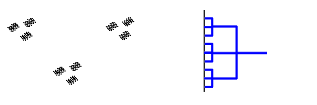
Figure 1. Dataset with multiscale structure and its corresponding dendrogram.

Ideally, users should be presented with a readily computable and presentable object which will give him/her the option of choosing the proper scale for the analysis, or perhaps interpreting the multiscale invariant directly, rather than being asked to choose a scale or choosing it for him/her. It is widely accepted that clustering is ultimately itself a tool for exploratory data analysis, [vLBD05]. In some sense, it is therefore totally acceptable to provide this multiscale invariant, whenever available and let the user pick different scale thresholds that will yield different partitions of the data. Once we accept this, we can concentrate on answering theoretical questions regarding schemes that output this kind of information. Our analysis will not, however, rule out clustering methods that provide a one-scale view of the data, since, formally, one can consider a such a scheme as one that at all scales gives the same information, cf. Example 2.2

We choose a particular way of representing this multiscale information, we use the formalism of persistent sets, which is introduced in Section 2, Definition 2.1. The idea of showing the multiscale clustering view of the dataset is widely used in Gene expression data analysis and it takes the form of dendrograms.

Functoriality: As our replacement for the constraints discussed in [Kle02], we will use instead the notion of functoriality which has been a very useful framework for the discussion of a variety of problems within mathematics over the last few decades. For a discussion of categories and functors, see [ML98]. Our idea is that clusters should be viewed as the stochastic analogue of the mathematical concept of path components. Recall (see, e.g. [Mun75]) that the path components of a topological space $X$ are the equivalence classes of points in the space under the equivalence relation $\sim_{path}$, where, for $x,y\in X$, we have $x\sim_{path}y$ if and only if there is a continuous map $\varphi:[0,1]\rightarrow X$ so that $\varphi(0)=x$ and $\varphi(1)=y$. In other words, two points in $X$ are in the same path component if they are connected by a continuous path in $X$. This set of components is denoted by $\pi_{0}(X)$. The assignment $X\rightarrow\pi_{0}(X)$ is said to be functorial, in that given a continuous map $f:X\rightarrow Y$ (morphism of topological spaces), there is a natural map of sets $\pi_{0}(f):\pi_{0}(X)\rightarrow\pi_{0}(Y)$, which is defined by requiring that $\pi_{0}(f)$ carries the path component of a point $x\in X$ to the path component of $f(x)\in Y$. This notion has been critical in many aspects of geometry; it provides the basis for the methods of organizing geometric objects combinatorially which is referred to as combinatorial or simplicial topology.

The input to clustering algorithms is not, of course, a topological space. Rather, it is typically point cloud data, finite sets of points lying in a Euclidean space of some dimension, or perhaps in some other metric space, such as a tree or a collection of words in some alphabet equipped with a metric. We will therefore think of it as a finite metric space (see [Mun75] for a discussion of metric spaces). There is a natural notion of what is meant by a map of metric spaces, which one can think of as loosely analogous to continuity. This notion has been used in other contexts in the past, see for example [Isb64]. Similarly, we define a natural notion of what is meant by a morphism of the persistent sets defined above, and require functoriality for the clustering algorithms we consider in terms of these notions of morphisms. For the time being the reader not familiar with the concept, can think of functoriality as a notion of coarse stability/consistency. By varying the richness of the class of morphisms between metric spaces one can control how stringent are the conditions imposed on the clustering algorithms. Functoriality can therefore be interpreted as a notion of coarse stability of these clustering algorithms.

In [McC02], the idea of using categorical and functorial ideas in statistics has been proposed as a formalism for defining what is meant by statistical models. One aspect of our work is to show that the same ideas, which are so powerful in many other aspects of mathematics, can be used to understand the nature of algorithms for accomplishing statistical tasks.

We summarize the main features of our point of view.

(a) It makes explicit the notion of multiscale representation of the set of clusters.

(b) By varying the degree of functoriality (i.e. by considering different notions of morphism on the domain of point cloud data) one can reason about the existence and properties of various schemes. We illustrate this possibility in Section 4. In particular, are able to prove a uniqueness theorem for clustering algorithms with one natural notion of functoriality.

(c) Beyond the conceptual advantages cited above, functoriality can be directly useful in analyzing datasets. The property can be used to study qualitative geometric properties of point cloud data, including more subtle geometric information than clustering, such as presence of “loopy” behavior or higher dimensional analogues. See e.g. [CIdSZ08] for an example of this point of view. We will also present an example in Subsection 3.2. In addition, the functoriality property can be used to analyze functions on the datasets, by studying the behavior of sublevel sets of the function under clustering. One version of this idea builds probabilistic versions of the Reeb graph. See [SMC07] for a number of examples of how this can work.

Other, different, notions of stability of clustering schemes have appeared in the literature, see [Rag82, BDvLP06] and references therein. We touch upon similar concepts in Section 5.

The organization of the paper is as follows. In Section 2 we introduce the main objects that model the output of clustering algorithms together with some important examples. Section 3 introduces the concepts of categories and functors, and the idea of functoriality is discussed. We present our main characterization results in Section 4. The quantitative study of stability and consistency is presented in Section 5. Further applications of the concept of functoriality are discussed in Section 6 and concluding remarks are presented in Section 7.

2. Persistence

In this section we define the objects which are the output of the clustering algorithms we will be working with. These objects will encode the notion of “multiscale” or “multiresolution” sets discussed in the introduction.

Let ${\mathcal{P}}(X)$ denote the set of partitions of the (finite) set $X$.

Definition 2.1.

A persistent set is a pair $(X,\theta)$, where $X$ is a finite set, and $\theta$ is a function from the non-negative real line $[0,+\infty)$ to ${\mathcal{P}}(X)$ so that the following properties hold.

1. If $r\leq s$, then $\theta(r)$ refines $\theta(s)$.

2. For any $r$, there is a number $\epsilon>0$ so that $\theta(r^{\prime})=\theta(r)$ for all $r^{\prime}\in[r,r+\epsilon]$.

If in addition there exists $t>0$ s.t. $\theta(t)$ consists of the single block partition for all $r\geq t$, then we say that $(X,\theta)$ is a dendrogram.

The intuition is that the set of blocks of the partition $\theta(r)$ should be regarded as $X$ viewed at scale $r$.

Example 2.1.

Let $(X,d)$ be a finite metric space. Then we can associate to $(X,d)$ the persistent set whose underlying set is $X$, and where blocks of the partition $\theta(r)$ consist of the equivalence classes under the equivalence relation $\sim_{r}$, where $x\sim_{r}x^{\prime}$ if and only if there is a sequence $x_{0},x_{1},\ldots,x_{t}\in X$ so that $x_{0}=x,x_{t}=x^{\prime}$, and $d(x_{i},x_{i+1})\leq r$ for all $i$.

Example 2.2.

A more trivial example is one in which $\theta(r)$ is constant, i.e. consists of a single partition. This is the scale free notion of clustering. Examples are $k$-means clustering and spectral clustering.

Example 2.3.

Here we consider the family of Agglomerative Hierarchical clustering techniques, [JD88]. We (re)define these by the recursive procedure described next. Let $X=\{x_{1},\ldots,x_{n}\}$ and let $\mathcal{L}$ denote a family of linkage functions, i.e. functions which one uses for defining the distance between two clusters. Fix $l\in{\mathcal{L}}$. For each $R>0$ consider the equivalence relation $\sim_{l,R}$ on blocks of a partition $\Pi\in{\mathcal{P}}(X)$, given by ${\mathcal{B}}\sim_{l,R}{\mathcal{B}}^{\prime}$ if and only if there is a sequence of blocks ${\mathcal{B}}={\mathcal{B}}_{1},\ldots,{\mathcal{B}}_{s}={\mathcal{B}}^{\prime}$ in $\Pi$ with $l({\mathcal{B}}_{k},{\mathcal{B}}_{k+1})\leq R$ for $k=1,\ldots,s-1$. Consider the sequences $r_{1},r_{2},\ldots\in[0,\infty)$ and $\Theta_{1},\Theta_{2},\ldots\in\mathcal{P}(X)$ given by $\Theta_{1}:=\{x_{1},\ldots,x_{n}\}$ and for $i\geq 1$, $\Theta_{i+1}=\Theta_{i}/\sim_{l,r_{i}}$ where $r_{i}:=\min\{l({\mathcal{B}},{\mathcal{B}}^{\prime}),\,{\mathcal{B}},{\mathcal{B}}^{\prime}\in\Theta_{i},\,{\mathcal{B}}\neq{\mathcal{B}}^{\prime}\}.$ Finally, we define $\theta^{l}:[0,\infty)\rightarrow\mathcal{P}(X)$ by $r\mapsto\theta^{l}(r):=\Theta_{i(r)}$ where $i(r):=\max\{i|r_{i}\leq r\}$. Standard choices for $l$ are single linkage: $l({\mathcal{B}},{\mathcal{B}}^{\prime})=\min_{x\in{\mathcal{B}}}\min_{x^{\prime}\in{\mathcal{B}}^{\prime}}d(x,x^{\prime});$ complete linkage $l({\mathcal{B}},{\mathcal{B}}^{\prime})=\max_{x\in{\mathcal{B}}}\max_{x^{\prime}\in{\mathcal{B}}^{\prime}}d(x,x^{\prime});$ and average linkage: $l({\mathcal{B}},{\mathcal{B}}^{\prime})=\frac{\sum_{x\in{\mathcal{B}}}\sum_{x^{\prime}\in{\mathcal{B}}^{\prime}}d(x,x^{\prime})}{\#{\mathcal{B}}\cdot\#{\mathcal{B}}^{\prime}}.$ It is easily verified that the notion discussed in Example 2.1 is equivalent to $\theta^{l}$ when $l$ is the single linkage function. Note that, unlike the usual definition of agglomerative hierarchical clustering, at each step of the inductive definition we allow for more than two clusters to be merged.

We will be using the persistent sets which arise out of Example 2.1. It is of course the case that the persistent set carries much more information than a single set of clusters. One can ask whether it carries too much information, in the sense that either (a) one cannot obtain useful interpretations from it or (b) it is computationally intractable. We claim that it can usually be usefully interpeted, and can be effectively and efficiently computed. One can observe this as follows. Since there are only a finite number of partitions of $X$, a persistent set ${\mathcal{Q}}$ gives a partition of $\mathbb{R}^{+}$ into a finite collection ${\mathcal{I}}$ of intervals of the form $[r,r^{\prime})$, together with one interval of the form $[r,+\infty)$. For each such interval, every number in the interval corresponds to the same partition of $X$.

We claim that knowledge of these intervals is a key piece of information about the persistent sets arising from Examples 2.1 and 2.3 above. The reason is that long intervals in ${\ I}$ correspond to large ranges of values of the scale parameter in which the associated cluster decomposition doesn’t change. One would then regard the partition into clusters corresponding to that interval as likely to represent significant structure present at the given range of scales. If there is only one long interval (aside from the infinite interval of the form $[r,+\infty)$) in ${\mathcal{I}}$, then one is led to believe that there is only one interesting range of scales, with a unique decomposition into clusters. However, if there are more that one long interval, then it suggests that the object has significant multiscale behavior, see Figure 1. Of course, the determination of what is “long” and what is “short” will be problem dependent, but choosing thresholds for the length of the intervals will give definite ranges of scales. As for the computability, the persistent sets associated to a finite metric space can be readily computed using (conveniently modified) hierarchical clustering techniques, or the methods of persistent homology (see [ZC04]).

3. Categories, functors and functoriality

3.1. Definitions and Examples

In this section, we will give a brief description of the theory of categories and functors, which will be the framework in which we state the constraints we will require of our clustering algorithms. An excellent reference for these ideas is [ML98].

Categories are useful mathematical constructs that encode the nature of certain objects of interest together with a set of admissible/interesting/useful maps between them. This formalism is extremely useful for studying classes of mathematical objects which share a common structure, such as sets, groups, vector spaces, or topological spaces. The definition is as follows.

Definition 3.1.

A category $\underline{C}$ consists of

• A collection of objects $ob(\underline{C})$ (e.g. sets, groups, vector spaces, etc.)

• For each pair of objects $X,Y\in ob(\underline{C})$, a set
  $Mor_{\underline{C}}(X,Y)$, the morphisms from $X$ to $Y$ (e.g. maps of sets from $X$ to $Y$, homomorphisms of groups from $X$ to $Y$, linear transformations from $X$ to $Y$, etc. respectively)

• Composition operations:
  $\mbox{\hskip 1.42271pt}\raisebox{1.13791pt}{\tiny{$\circ$ }}:Mor_{\underline{C}}(X,Y)\times Mor_{\underline{C}}(Y,Z)\rightarrow Mor_{\underline{C}}(X,Z)$, corresponding to composition of set maps, group homomorphisms, linear transformations, etc.

• For each object $X\in\underline{C}$, a distinguished element $id_{X}\in Mor_{\underline{C}}(X,X)$

The composition is assumed to be associative in the obvious sense, and for any $f\in Mor_{\underline{C}}(X,Y)$, it is assumed that $id_{Y}\mbox{\hskip 1.42271pt}\raisebox{1.13791pt}{\tiny{$\circ$ }}f=f$ and $f\mbox{\hskip 1.42271pt}\raisebox{1.13791pt}{\tiny{$\circ$ }}id_{X}=f$.

Here are the relevant examples for this paper.

Example 3.1.

We will construct three categories $\underline{{\mathcal{M}}}^{iso}$, $\underline{{\mathcal{M}}}^{mon}$, and $\underline{{\mathcal{M}}}^{gen}$, whose collections of objects will all consist of the collection of finite metric spaces. Let $(X,d_{X})$ and $(Y,d_{Y})$ denote finite metric spaces. A set map $f:X\rightarrow Y$ is said to be distance non increasing if for all $x,x^{\prime}\in X$, we have $d_{Y}(f(x),f(x^{\prime}))\leq d_{X}(x,x^{\prime})$. It is easy to check that composition of distance non-increasing maps are also distance non-increasing, and it is also clear that $id_{X}$ is always distance non-increasing. We therefore have the category $\underline{{\mathcal{M}}}^{gen}$, whose objects are finite metric spaces, and so that for any objects $X$ and $Y$, $Mor_{\underline{{\mathcal{M}}}^{gen}}(X,Y)$ is the set of distance non-increasing maps from $X$ to $Y$, cf. [Isb64] for another use of this class of maps. We say that a distance non-increasing map is monic if it is an inclusion as a set map. It is clear compositions of monic maps are monic, and that all identity maps are monic, so we have the new category $\underline{{\mathcal{M}}}^{mon}$, in which $Mor_{\underline{{\mathcal{M}}}^{mon}}(X,Y)$ consists of the monic distance non-increasing maps. Finally, if $(X,d_{X})$ and $(Y,d_{Y})$ are finite metric spaces, $f:X\rightarrow Y$ is an isometry if $f$ is bijective and $d_{Y}(f(x),f(x^{\prime}))=d_{X}(x,x^{\prime})$ for all $x$ and $x^{\prime}$. It is clear that as above, one can form a category $\underline{{\mathcal{M}}}^{iso}$ whose objects are finite metric spaces and whose morphisms are the isometries. It is clear that we have inclusions

(3–1) $$\underline{{\mathcal{M}}}^{iso}\subseteq\underline{{\mathcal{M}}}^{mon}\subseteq\underline{{\mathcal{M}}}^{gen}$$

of subcategories (defined as in [ML98]). Note that although the inclusions are bijections on object sets, they are proper inclusions on morphism sets, i.e. they are not in general surjective.

We will also construct a category of persistent sets.

Example 3.2.

Let $(X,\theta),(Y,\eta)$ be persistent sets. For any partition $\Pi$ of a set $Y$, and any set map $f:X\rightarrow Y$, we define $f^{*}(\Pi)$ to be the partition of $X$ whose blocks are the sets $f^{-1}({\mathcal{B}})$, as ${\mathcal{B}}$ ranges over the blocks of $\Pi$. A map of sets $f:X\rightarrow Y$ is said to be persistence preserving if for each $r\in\mathbb{R}$, we have that $\theta(r)$ is a refinement of $f^{*}(\eta(r))$. It is easily verified that the composite of persistence preserving maps is persistence preserving, and that any identity map is persistence preserving, and it is therefore clear that we may define a category $\underline{{\mathcal{P}}}$ whose objects are persistent sets, and where $Mor_{\underline{{\mathcal{P}}}}((X,\theta),(Y,\eta))$ consists of the set maps from $X$ to $Y$ which are persistence preserving. A simple example is shown in Figure 2.

Figure 2. Two persistent sets $(X,\theta)$ and $(Y,\eta)$ represented by their dendrograms. On the left one defined in the set $X=\{A,B,C\}$ and on the right one defined on the set $Y=\{A^{\prime},B^{\prime},C^{\prime}\}$. Consider the given set map $f:X\rightarrow Y$. Then we see that $f$ is persistence preserving since for each $r\geq 0$, the partition $\theta(r)$ is a refinement of $f^{*}(\eta(r))$. Indeed, there are three interesting ranges of values of $r$. Pick for example $r$ like in the orange shaded area: $r\in[1,2)$. Then $\eta(r)=\{\{A^{\prime},B^{\prime}\},\{C^{\prime}\}\}$ and hence $f^{*}(\eta(r))=\{f^{-1}(\{A^{\prime},B^{\prime}\}),\{f^{-1}(C^{\prime})\}\}=\{\{A,B\},\{C\}\}$ which is indeed refined by $\theta(r)=\{\{A\},\{B\},\{C\}\}$. One proceeds similary for the other two cases.

We next introduce the key concept in our discussion, that of a functor. We give the formal definition first.

Definition 3.2.

Let $\underline{C}$ and $\underline{D}$ be categories. Then a functor from $\underline{C}$ to $\underline{D}$ consists of

• A map of sets $F:ob(\underline{C})\rightarrow ob(\underline{D})$

• For every pair of objects $X,Y\in\underline{C}$ a map of sets $\Phi(X,Y):Mor_{\underline{C}}(X,Y)\rightarrow Mor_{\underline{D}}(FX,FY)$ so that

  1. $\Phi(X,X)(id_{X})=id_{F(X)}$ for all $X\in ob(\underline{C})$

  2. $\Phi(X,Z)(g\mbox{\hskip 1.42271pt}\raisebox{1.13791pt}{\tiny{$\circ$ }}f)=\Phi(Y,Z)(g)\mbox{\hskip 1.42271pt}\raisebox{1.13791pt}{\tiny{$\circ$ }}\Phi(X,Y)(f)$ for all $f\in Mor_{\underline{C}}(X,Y)$ and $g\in Mor_{\underline{C}}(Y,Z)$

Remark 3.1.

In the interest of clarity, we often refer to the pair $(F,\Phi)$ as a single letter $F$. See diagram (3–2) in Example 3.5 below for an example.

A morphism $f:X\rightarrow Y$ which has a two sided inverse $g:Y\rightarrow X$, so that $f\mbox{\hskip 1.42271pt}\raisebox{1.13791pt}{\tiny{$\circ$ }}g=id_{Y}$ and $g\mbox{\hskip 1.42271pt}\raisebox{1.13791pt}{\tiny{$\circ$ }}f=id_{X}$, is called an isomorphism. Two objects which are isomorphic are intuitively thought of as “structurally indistinguishable” in the sense that they are identical except for naming or choice of coordinates. For example, in the category of sets, the sets $\{1,2,3\}$ and $\{A,B,C\}$ are isomorphic, since they are identical except for choice made in labelling the elements. We illustrate this definition with some examples.

Example 3.3.

(Forgetful functors) When one has two categories $\underline{C}$ and $\underline{D}$, where the objects in $\underline{C}$ are objects in $\underline{D}$ equipped with some additional structure and the morphisms in $\underline{C}$ are simply the morphisms in $\underline{D}$ which preserve that structure, then we obtain the “forgetful functor” from $\underline{C}$ to $\underline{D}$, which carries the object in $\underline{C}$ to the same object in $\underline{C}$, but regarded without the additional structure. For example, a group can be regarded as a set with the additional structure of multiplication and inverse maps, and the group homomorphisms are simply the set maps which respect that structure. Accordingly, we have the functor from the category of groups to the category of sets which “forgets the multiplication and inverse”. Similarly, we have the forgetful functor from $\underline{{\mathcal{P}}}$ to the category of sets, which forgets the presence of $\theta$ in the persistent set $(X,\theta)$.

Example 3.4.

The inclusions $\underline{{\mathcal{M}}}^{iso}\subseteq\underline{{\mathcal{M}}}^{mon}\subseteq\underline{{\mathcal{M}}}^{gen}$ are both functors.

Any given clustering scheme is a procedure $F$ which takes as input a finite metric space $(X,d_{X})$, that is, an object in $ob(\underline{\mathcal{M}}^{gen})$, and delivers as output a persistent set, that is, an object in $ob(\underline{\mathcal{P}})$. The concept of functoriality refers to the additional condition that the clustering procedure maps a pair of input objects into a pair of output objects in a manner which is consistent/stable with respect to the morphisms attached to the input and output spaces. When this happens, we say that the clustering scheme is functorial. This notion of consistency/stability is made precise in Definition 3.2 and described by diagram (3–2).

Now, the idea is to regard clustering algorithms (that output a persistent set) as functors. Assume for instance we want to consider “stability” to all distance non-increasing maps. Then the correct category of inputs (finite metric spaces) is $\underline{{\mathcal{M}}}^{gen}$ and the category of outputs is $\underline{\mathcal{P}}$. According to Definition 3.2 in order to view a clustering scheme as a functor we need to specify (1) how it maps objects of $\underline{{\mathcal{M}}}^{gen}$ (finite metric spaces) into objects of $\underline{\mathcal{P}}$ (persistent sets), and (2) how a valid morphism/map $f:(X,d_{X})\rightarrow(Y,d_{Y})$ between two objects $(X,d_{X})$ and $(Y,d_{Y})$ in the input space/category $\underline{{\mathcal{M}}}^{gen}$ induce a map in the output category $\underline{\mathcal{P}}$, see diagram (3–2) below.

We exemplify this through the construction of the key example for this paper.

Example 3.5.

We define a functor

$${\mathcal{R}}^{gen}:\underline{{\mathcal{M}}}^{gen}\rightarrow\underline{{\mathcal{P}}}$$

as follows. For a finite metric space $(X,d_{X})$, we define ${\mathcal{R}}^{gen}(X,d_{X})$ to be the persistent set $(X,\theta^{d_{X}})$, where $\theta^{d_{X}}(r)$ is the partition associated to the equivalence relation $\sim_{r}$ defined in Example 2.1. This is clearly an object in $\underline{{\mathcal{P}}}$. We also define how ${\mathcal{R}}^{gen}$ acts on maps $f:(X,d_{X})\rightarrow(Y,d_{Y})$: The value of ${\mathcal{R}}^{gen}(f)$ is simply the set map $f$ regarded as a morphism from $(X,\theta^{d_{X}})$ to $(Y,\theta^{d_{Y}})$ in $\underline{{\mathcal{P}}}$. That it is a morphism in $\underline{{\mathcal{P}}}$ is easy to check. This functorial construction is represented through the diagram below:

(3–2)

where ${\mathcal{R}}^{gen}(f)$ is persistence preserving.

Example 3.6.

By restricting ${\mathcal{R}}^{gen}$ to the subcategories $\underline{{\mathcal{M}}}^{iso}\mbox{ and }\underline{{\mathcal{M}}}^{mon}$, we obtain functors
${\mathcal{R}}^{iso}:\underline{{\mathcal{M}}}^{iso}\rightarrow\underline{{\mathcal{P}}}$ and ${\mathcal{R}}^{mon}:\underline{{\mathcal{M}}}^{mon}\rightarrow\underline{{\mathcal{P}}}$.

Example 3.7.

Let $\lambda$ be any positive real number. Then we define a functor $\sigma_{\lambda}:\underline{{\mathcal{M}}}^{gen}\rightarrow\underline{{\mathcal{M}}}^{mon}$ on objects by

$$\sigma_{\lambda}(X,d_{X})=(X,\lambda d_{X})$$

and on morphisms by $\sigma_{\lambda}(f)=f$. One easily verifies that if $f$ satisfies the conditions for being a morphism in $\underline{{\mathcal{M}}}^{gen}$ from $(X,d_{X})$ to $(Y,d_{Y})$, then it readily satisfies the conditions to be a morphism from $(X,\lambda d_{X})$ to $(Y,\lambda d_{Y})$. Similarly, we define a functor $s_{\lambda}:\underline{{\mathcal{P}}}\rightarrow\underline{{\mathcal{P}}}$ by setting $s_{\lambda}(X,\theta)=(X,\theta^{\lambda})$, where $\theta^{\lambda}(r)=\theta(\frac{r}{\lambda})$.

In Section 4 we will be showing our main results. We will now have a brief disgression to discuss other situations in which, in our opinion, the concept of functoriality can be useful.

3.2. Intrinsic Value of Functoriality

By studying functorial methods of clustering, it is possible to recover qualitative aspects of the geometric structure of a dataset. We illustrate this idea with a “toy” example. We suppose that we have a point cloud data which is concentrated around the unit circle. We consider the projection of the data on to the $x$-axis, and cover the axis with two (overlapping) intervals $U$ and $V$, pictured on the left in Figure 3 below as being red and yellow, with orange intersection. By considering those portions of the dataset whose $x$-coordinate lie in $U$ and $V$ respectively, we obtain the red and yellow subsets of the dataset pictured on the right below. Their intersection is pictured as orange, and the arrows indicate that we have inclusions of the intersection into each of the pieces.

Figure 3. Left: Covering of a circle by two intervals. Center: Corresponding diagram of components. Right: Homotopy colimit of diagram in center figure.

Next, we note that if we are dealing with a functorial clustering scheme, and cluster each of these subsets, we obtain the diagram of clusters in the center of Figure 3. This is now a very simple combinatorial object.

There is a topological construction known as the homotopy colimit, which given any diagram of sets of any shape reconstructs a simplicial set (a slightly more flexible version of the notion of simplicial complex), and in particular a space. To first approximation, one builds a vertex for every element in any set in the diagram, and an edge between any two elements which are connected by a map in the diagram, and then attaches higher order simplices according to a well defined procedure. In the case of the diagram above, this constructs the space given in the rightmost part of Figure 3 .

The details of the theory of simplicial sets and homotopy colimits are beyond the scope of this paper. A thorough exposition is given in [BK72].

Functoriality is also quite useful when one is interested in studying the qualitative behavior of a real-valued function $f$ on a dataset, for example the output of a density estimator. Then it is useful to study the set of clusters in sublevel and superlevel sets of $f$, and understanding how the clusters behave under changes in the thresholds can help one understand the presence of saddle points and higher index critical points of the function.

One example of this is two-parameter persistence constructions, [CSZon]. In this case, there is more structure than just persistent sets (trees/dendrograms) as defined in this paper.

We will elaborate on another application of functoriality in Section 6.

4. Results

We now study different clustering algorithms using the idea of functoriality. We have 3 possible “input” categories ordered by inclusion (3–1). The idea is that studying functoriality over a larger category will be more stringent/demanding than requiring functoriality over a smaller one. We now consider different clustering algorithms and study whether they are functorial over our choice of the input category. We start by analyzing functoriality over the least demanding one, $\underline{\mathcal{M}}^{iso}$, then we prove a uniqueness result for functoriality over $\underline{\mathcal{M}}^{gen}$ and finally we study how relaxing the conditions imposed by the morphisms in $\underline{\mathcal{M}}^{gen}$, namely, by restricting ourselves to the smaller but intermediate category $\underline{\mathcal{M}}^{mon}$, we permit more functorial clustering algorithms.

4.1. Functorality over $\underline{{\mathcal{M}}}^{iso}$

This is the smallest category we will deal with. The morphisms in $\underline{{\mathcal{M}}}^{iso}$ are simply the bijective maps between datasets which preserve the distance function. As such, functoriality of a clustering algorithms over $\underline{{\mathcal{M}}}^{iso}$ simply means that the output of the scheme doesn’t depend on any artifacts in the dataset, such as the way the points are named or the way in which they are ordered. Here are some examples which illustrate the idea.

• The $k$-means algorithm (see [JD88]) is in principle allowed by our framework since $ob(\underline{\mathcal{P}})$ contains all constant persistent sets. However it is not functorial on any of our input categories. It depends both on a paramter $k$ (number of clusters) and on an initial choices of means, and is not therefore dependent on the metric structure alone.

• Agglomerative hierarchical clustering, in standard form, as described for example in [JD88], begins with point cloud data and constructs a binary tree (or dendrogram) which describes the merging of clusters as a threshold is increased. The lack of functoriality comes from the fact that when a single threshold value corresponds to more than one data point, one is forced to choose an ordering in order to decide which points to “agglomerate” first. This can easily be modified by relaxing the requirement that the tree be binary. This is what we did in Example 2.3 In this case, one can view these methods as functorial on $\underline{{\mathcal{M}}}^{iso}$, where the functor takes its values in arbitrary rooted trees. It is understood that in this case, the notion of morphism for the output ($\underline{\mathcal{P}}$) is simply isomorphism of rooted trees. In contrast, we see next that amongst these methods, when we impose that they be functorial over the larger (more demanding) category $\underline{\mathcal{M}}^{gen}$ then only one of them passes the test.

• Spectral clustering. As described in [vL07], typically, spectral methods consist of two different layers. They first define a laplacian matrix out of the dissimilarity matrix (given by $d_{X}$ in our case) and then find eigenvalues and eigenvectors of this operator. The second layer is as follows: a natural number $k$ must be specified, a projection to $\mathbb{R}^{k}$ is performed using the eigenfunctions, and clusters are found by an application of the $k$-means clustering algorithm. Clearly, operations in the second layer will fail to be functorial as they do not depend on the metric alone. However, the procedure underlying in the first layer is clearly functorial on $\underline{\mathcal{M}}^{iso}$ as eigenvalue computations are changed by a permutation in a well defined, natural, way.

4.2. Functorality over $\underline{\mathcal{M}}^{gen}$: a uniqueness theorem

In this section, as an example application of the conceptual framework of functoriality, we will prove a theorem of the same flavor as the main theorem of [Kle02], except that we prove existence and uniqueness on $\underline{\mathcal{M}}^{gen}$ instead of impossibility in our context.

Before stating and proving our theorem, it is interesting to point out why complete linkage and average linkage (agglomerative) clustering, as defined in Example 2.3 are not functorial on $\underline{\mathcal{M}}^{gen}$. A simple example explains this: consider the metric spaces $X=\{A,B,C\}$ with metric given by the edge lengths $\{4,3,5\}$ and $Y=(A^{\prime},B^{\prime},C^{\prime})$ with metric given by the edge lengths $\{4,3,2\}$, as given in Figure 4. Obviously the map $f$ from $X$ to $Y$ with $f(A)=A^{\prime}$, $f(B)=B^{\prime}$ and $f(C)=C^{\prime}$ is a morphism in $\underline{\mathcal{M}}^{gen}$. Note that for example for $r=3.5$ (shaded regions of the dendrograms in Figure 4) we have that the partition of $X$ is $\Pi_{X}=\{\{A,C\},B\}$ whereas the partition of $Y$ is $\Pi_{Y}=\{\{A^{\prime},B^{\prime}\},C^{\prime}\}$ and thus $f^{*}(\Pi_{Y})=\{\{A,B\},\{C\}\}$. Therefore $\Pi_{X}$ does not refine $f^{*}(\Pi_{Y})$ as required by functoriality. The same construction yields a counter-example for average linkage.

Figure 4. An example that shows why complete linkage fails to be functorial on $\underline{\mathcal{M}}^{gen}$.

Theorem 4.1.

Let $\Psi:\underline{{\mathcal{M}}}^{gen}\rightarrow\underline{{\mathcal{P}}}$ be a functor which satisfies the following conditions.

(I):

Let $\alpha:\underline{{\mathcal{M}}}^{gen}\rightarrow\underline{Sets}$ and $\beta:\underline{{\mathcal{P}}}\rightarrow\underline{Sets}$ be the forgetful functors$(X,d_{X})\rightarrow X$ and $(X,\theta)\rightarrow X$, which forget the metric and partition respectively, and only “remember” the underlying sets $X$. Then we assume that $\beta\mbox{\hskip 1.42271pt}\raisebox{1.13791pt}{\tiny{$\circ$ }}\Psi=\alpha$. This means that the underlying set of the persistent set associated to a metric space is just the underlying set of the metric space.

(II):

For $\delta\geq 0$ let $Z(\delta)=(\{p,q\},\left(\begin{smallmatrix}0&{\delta}\\ {\delta}&0\end{smallmatrix}\right))$ denote the two point metric space with underlying set $\{p,q\}$, and where $\mbox{dist}(p,q)=\delta$. Then $\Psi(Z(\delta))$ is the persistent set $(\{p,q\},\theta^{Z(\delta)})$ whose underlying set is $\{p,q\}$ and where $\theta^{Z(\delta)}(t)$ is the partition with one element blocks when $t<\delta$ and it is the partition with a single two point block when $t\geq\delta$.

(III):

Given a finite metric space $(X,d_{X})$, let

$$\mbox{sep}(X):=\min_{x\neq x^{\prime}}d_{X}(x,x^{\prime}).$$

Write $\Psi(X,d_{X})=(X,\theta^{\Psi})$, then for any $t<\mbox{sep}(X)$, the partition $\theta^{\Psi}(t)$ is the discrete partition with one element blocks.

Then $\Psi$ is equal to the functor ${\mathcal{R}}^{gen}$.

Proof.

Let $\Psi(X,d_{X})=(X,\theta^{\Psi})$. For each $r\geq 0$ we will prove that (a) $\theta^{d_{X}}(r)$ is a refinement of $\theta^{\Psi}(r)$ and (b) $\theta^{\Psi}(r)$ is a refinement of $\theta^{d_{X}}(r)$.

Then it will follow that $\theta^{d_{X}}(r)=\theta^{\Psi}(r)$ for all $r\geq 0$, which shows that the objects are the same. Since this is a situation where, given any pair of objects, there is at most one morphism between them, this also determines the effect of the functor on morphisms.

Fix $r\geq 0$. In order to obtain (a) we need to prove that whenever $x,x^{\prime}\in X$ lie in the same block of the partition $\theta^{d_{X}}(r)$, that is $x\sim_{r}x^{\prime}$, then they both lie in the same block of $\theta^{\Psi}(r)$.

It is enough to prove the following Claim: whenever
$d_{X}(x,x^{\prime})\leq r$ then $x$ and $x^{\prime}$ lie in the same block of $\theta^{\Psi}(r)$.

Indeed, if the claim is true, and $x\sim_{r}x^{\prime}$ then one can find $x_{0},x_{1},\ldots,x_{n}$ with $x_{0}=x$, $x_{n}=x^{\prime}$ and $d_{X}(x_{i},x_{i+1})\leq r$ for $i=0,1,2,\ldots,n-1$. Then, invoking the claim for all pairs $(x_{i},x_{i+1})$, $i=0,\ldots,n-1$ one would find that: ${x}=x_{0}$ and $x_{1}$ lie in the same block of $\theta^{\Psi}(r)$, $x_{1}$ and $x_{2}$ lie in the same block of $\theta^{\Psi}(r)$, $\ldots$, $x_{n-1}$ and $x_{n}=x^{\prime}$ lie in the same block of $\theta^{\Psi}(r)$. Hence, $x$ and $x^{\prime}$ lie in the same block of $\theta^{\Psi}(r)$.

So, let’s prove the claim. Assume $d_{X}(x,x^{\prime})\leq r$, then the function given by $p\rightarrow x,q\rightarrow x^{\prime}$ is a morphism $g:Z(r)\rightarrow(X,d_{X})$ in $\underline{{\mathcal{M}}}^{gen}$. This means that we obtain a morphism

$$\Psi(g):\Psi(Z(r))\rightarrow\Psi(X,d_{X})$$

in $\underline{{\mathcal{P}}}$. But, $p$ and $q$ lie in the same block of the partition $\theta^{Z(r)}$ by definition of $Z(r)$, and functoriality therefore guarantees that $\Psi(g)$ is persistence preserving (recall Example 3.2) and hence the elements $g(p)=x$ and $g(q)=x^{{\prime}}$ lie in the same block of $\theta^{d_{X}}(r)$. This concludes the proof of (a).

For condition (b), assume that $x$ and $x^{\prime}$ belong to the same block of the partition $\theta^{\Psi}(r)$. We will prove that necessarily $x\sim_{r}x^{\prime}$. This of course will imply that $x$ and $x^{\prime}$ belong to the same block of $\theta^{d_{X}}(r)$.

Consider the metric space $(X[r],d_{[r]})$ whose points are the equivalence classes of $X$ under the equivalence relation $\sim_{r}$, and where the metric $d_{[r]}:X[r]\times X[r]\rightarrow\mathbb{R}^{+}$ is defined to be the maximal metric pointwisely less than or equal to $W$, where for two points ${\mathcal{B}}$ and ${\mathcal{B}}^{\prime}$ in $X[r]$ (equivalence classes of $X$ under $\sim_{r}$), $W({\mathcal{B}},{\mathcal{B}}^{\prime})=\min_{x\in{\mathcal{B}}}\min_{x^{\prime}\in{\mathcal{B}}^{\prime}}d_{X}(x,x^{\prime}).$ It follows from the definition of $\sim_{r}$ that if two equivalence classes are distinct, then the distance between them is $>r$. This means that $\mbox{sep}(X[r])>r.$

Write $\Psi(X[r],d_{[r]})=(X[r],\theta^{[r]})$. Since $\mbox{sep}(X[r])>r$, hypothesis (III) now directly shows that the blocks of the partition $\theta^{[r]}(r)$ are exactly the equivalence classes of $X$ under the equivalence relation $\sim_{r}$, that is $\theta^{[r]}(r)=\theta^{d_{X}}(r)$. Finally, consider the morphism

$$\pi_{r}:(X,d_{X})\rightarrow(X[r],d_{[r]})$$

in $\underline{{\mathcal{M}}}^{gen}$ given on elements $x\in X$ by $\pi_{r}(x)=[x]_{r}$, where $[x]_{r}$ denotes the equivalence class of $x$ under $\sim_{r}$. By functoriality, $\Psi(\pi_{r}):(X,\theta^{\Psi})\rightarrow(X[r],\theta^{[r]})$ is persistence preserving, and therefore, $\theta^{\Psi}(r)$ is a refinement of $\theta^{[r]}(r)=\theta^{d_{X}}(r)$. This is depicted as follows:

This concludes the proof of (b). ∎

We should point out that another characterization of single linkage has been obtained in the book [JS71].

4.2.1. Comments on Kleinberg’s conditions

We conclude this section by observing that analogues of the three (axiomatic) properties considered by Kleinberg in [Kle02] hold for ${\mathcal{R}}^{gen}$.

Kleinberg’s first condition was scale-invariance, which asserted that if the distances in the underlying point cloud data were multiplied by a constant positive multiple $\lambda$, then the resulting clustering decomposition should be identical. In our case, this is replaced by the condition that ${\mathcal{R}}^{gen}\mbox{\hskip 1.42271pt}\raisebox{1.13791pt}{\tiny{$\circ$ }}\sigma_{\lambda}(X,d_{X})=s_{\lambda}\mbox{\hskip 1.42271pt}\raisebox{1.13791pt}{\tiny{$\circ$ }}{\mathcal{R}}^{gen}(X,d_{X})$, which is trivially satisfied.

Kleinberg’s second condition, richness, asserts that any partition of a dataset can be obtained as the result of the given clustering scheme for some metric on the dataset. In our context, partitions are replaced by persistent sets. Assume that there exist $t\in\mathbb{R}$ s.t. $\theta(t)$ is the single block partition, i.e., impose that the persistent set is a dendrogram (cf. Definition 2.1). In this case, it is easy to check that any such persistent set can be obtained as ${\mathcal{R}}^{gen}$ evaluated for some (pseudo)metric on some dataset. Indeed, let $(X,\theta)\in{ob}(\underline{\mathcal{P}})$. Let $\epsilon_{1},\ldots,\epsilon_{k}$ be the (finitely many) transition/discontinuity points of $\theta$. For $x,x^{\prime}\in X$ define $d_{X}(x,x^{\prime})=\min\{\epsilon_{i}\}$ s.t. $x,x^{\prime}$ belong to same block of $\theta(\epsilon_{i})$.

This is a pseudo metric on $X$. Indeed, pick points $x,x^{\prime}$ and $x^{\prime\prime}$ in $X$. Let $\epsilon_{1}$ and $\epsilon_{2}$ be minimal s.t. $x,x^{\prime}$ belong to the same block of $\theta(\epsilon_{1})$ and $x^{\prime},x^{\prime\prime}$ belong to the same block of $\theta(\epsilon_{2})$. Let $\epsilon_{12}:=\max(\epsilon_{1},\epsilon_{2})$. Since $(X,\theta)$ is a persistent set (Definition 2.1), $\theta(\epsilon_{12})$ must have a block $\mathcal{B}$ s.t. $x,x^{\prime}$ and $x^{\prime\prime}$ all lie in $\mathcal{B}$. Hence $d_{X}(x,x^{\prime\prime})\leq\epsilon_{12}\leq\epsilon_{1}+\epsilon_{2}=d_{X}(x,x^{\prime})+d_{X}(x^{\prime},x^{\prime\prime})$.

Finally, Kleinberg’s third condition, consistency, could be viewed as a rudimentary example of functoriality. His morphisms are similar to the ones in $\underline{\mathcal{M}}^{gen}$.

4.3. Functoriality over $\underline{{\mathcal{M}}}^{mon}$

In this section, we illustrate how relaxing the functoriality permits more clustering algorithms. In other words, we will restrict ourselves to $\underline{{\mathcal{M}}}^{mon}$ which is smaller (less stringent) than $\underline{{\mathcal{M}}}^{gen}$ but larger (more stringent) than $\underline{{\mathcal{M}}}^{iso}$. We consider the restriction of ${\mathcal{R}}^{gen}$ to the category $\underline{{\mathcal{M}}}^{mon}$. For any metric space and every value of the persistence parameter $r$, we will obtain a partition of the underlying set $X$ of the metric space in question, and the set of equivalence classes under $\sim_{r}$. For any $x\in X$, let $[x]_{r}$ be the equivalence class of $x$ under the equivalence relation $\sim_{r}$, and define $c(x)=\#[x]_{r}$. For any integer $m$, we now define $X_{m}\subseteq X$ by $X_{m}=\{x\in X|c(x)\geq m\}$. We note that for any morphism $f:X\rightarrow Y$ in $\underline{{\mathcal{M}}}^{mon}$, we find that $f(X_{m})\subseteq Y_{m}$. This property clearly does not hold for more general morphisms. For every $r$, we can now define a new equivalence relation $\sim^{m}_{r}$ on $X$, which refines $\sim_{r}$, by requiring that each equivalence class of $\sim_{r}$ which has cardinality $\geq m$ is an equivalence class of $\sim_{r}^{m}$, and that for any $x$ for which $c(x)<m$, $x$ defines a singleton equivalence class in $\sim^{m}_{r}$. We now obtain a new persistent set $(X,\theta^{m})$, where $\theta^{m}(r)$ will denote the partition associated to the equivalence relation $\sim^{m}_{r}$. It is readily checked that $X\rightarrow(X,\theta^{m})$ is functorial on $\underline{{\mathcal{M}}}^{mon}$. This scheme could be motivated by the intuitition that one does not regard clusters of small cardinality as significant, and therefore makes points lying in small clusters into singletons, where one can then remove them as representing “outliers”.

5. Metric stability and convergence properties of ${\mathcal{R}}^{gen}$

In this section we briefly discuss some further properties of ${\mathcal{R}}^{gen}$ (single linkage dendrograms). We will provide quantitative results on the stability and convergence/consitency properties of this functor (algorithm). To the best of our knowledge, the only other related results obtained for this algorithm appear in [Har81]. The issues of stability and convergence/consistency of clustering algorithms have brought back into attention recently, see [vLBD05, BDvLP06] and references therein. In Theorem 5.1 besides proving stability, we prove convergence in a simple setting.

Given finite metric spaces $(X,d_{X})$ and $(Y,d_{Y})$, our goal is to define a distance between the persistence objects $\theta^{d_{X}}$ and $\theta^{d_{Y}}$ respectively produced by ${\mathcal{R}}^{gen}$. We know that this functor actually outputs dendrograms (rooted trees), which have a natural metric structure attached to them. Moroever, it is well known that rooted trees are uniquely characterized by their distance matrix, [SS03].

For a finite metric space $(X,d_{X})$ consider the derived metric space $(X,\varepsilon_{X})$ with the same underlying set and metric

(5–3) $$\varepsilon_{X}(x,x^{\prime}):=\min\{\varepsilon\geq 0|\,x\sim_{\varepsilon}x^{\prime}\}.$$

Note that $(X,\theta^{d_{X}})$ can therefore obviously be regarded as the metric space $(X,\varepsilon_{X})$, cf. with the construction of the metric in section 4.2.1. We now check that indeed $\varepsilon_{X}$ defines a metric on $X$.

Proposition 5.1.

For any finite metric space $(X,d_{X})$, $(X,\varepsilon_{X})$ is also a metric space.

Proof.

(a) Since $d_{X}$ is a metric on $X$, it is obvious that $\varepsilon_{X}(x,x^{\prime})=0$ implies $x=x^{\prime}$. (b) Symmetry is also obvious since $\sim_{\varepsilon}$ is an equivalence relation. (c) Triangle inequality: Pick $x,x^{\prime},x^{\prime\prime}\in X$. Let $\varepsilon_{X}(x,x^{\prime})=\varepsilon_{1}$ and $\varepsilon_{X}(x^{\prime},x^{\prime\prime})=\varepsilon_{2}$. Then, there exist points $a_{0},a_{1},\ldots,a_{j}$ and $b_{0},b_{1},\ldots,b_{k}$ in $X$ with $a_{0}=x$, $a_{j}=x^{\prime}=b_{0}$, $b_{k}=x^{\prime\prime}$ and $d_{X}(a_{i},a_{i+1})\leq\varepsilon_{1}$ for $i=0,\ldots,j-1$ and $d_{X}(b_{i},b_{i+1})\leq\varepsilon_{2}$ for $i=0,\ldots,k-1$. Consider the points $\{c_{i}\}_{i=0}^{j+k+1}=\{a_{0},\ldots,a_{j},b_{1},\ldots,b_{k}\}.$
Then $d_{X}(c_{i},c_{i+1})\leq\max(\varepsilon_{1},\varepsilon_{2})\leq\varepsilon_{1}+\varepsilon_{2}$. Hence $x\sim_{\varepsilon_{12}}x^{\prime\prime}$ with $\varepsilon_{12}=\varepsilon_{1}+\varepsilon_{2}$ and then by definition (5–3), $\varepsilon_{X}(x,x^{\prime\prime})\leq\varepsilon_{X}(x,x^{\prime})+\varepsilon_{X}(x^{\prime},x^{\prime\prime}).$ ∎

In order to compare the outputs of ${\mathcal{R}}^{gen}$ on two different finite metric spaces $(X,d_{X})$ and $(X^{\prime},d_{X^{\prime}})$ we will instead compare the metric space representations of those outputs, $(X,\varepsilon_{X})$ and $(X^{\prime},\varepsilon_{X^{\prime}})$, respectively. For this purpose, we choose to work with the Gromov-Hausdorff distance which we define now, [BBI01].

Definition 5.1 (Correspondence).

For sets $A$ and $B$, a subset $R\subset A\times B$ is a correspondence (between $A$ and $B$) if and and only if

• $\forall$ $a\in A$, there exists $b\in B$ s.t. $(a,b)\in R$

• $\forall$ $b\in B$, there exists $a\in X$ s.t. $(a,b)\in R$

Let ${\mathcal{R}}(A,B)$ denote the set of all possible correspondences between sets $A$ and $B$.

Consider finite metric spaces $(X,d_{X})$ and $(Y,d_{Y})$. Let $\Gamma_{X,Y}:X\times Y\bigtimes X\times Y\rightarrow\mathbb{R}^{+}$ be given by

$$(x,y,x^{\prime},y^{\prime})\mapsto|d_{X}(x,x^{\prime})-d_{Y}(y,y^{\prime})|.$$

Then, the Gromov-Hausdorff distance between $X$ and $Y$ is given by

(5–4) $$d_{\mathcal{G}\mathcal{H}}({X},{Y}):=\inf_{R\in{\mathcal{R}}(X,Y)}\,\,\max_{(x,y),(x^{\prime},y^{\prime})\in R}\Gamma_{X,Y}(x,y,x^{\prime},y^{\prime})$$

Remark 5.1.

This expression defines a metric on the set of (isometry classes of) finite metric spaces, [BBI01] (Theorem 7.3.30).

One has:

Proposition 5.2.

For any finite metric spaces $(X,d_{X})$ and $(Y,d_{Y})$

$$d_{\mathcal{G}\mathcal{H}}({(X,d_{X})},{(Y,d_{Y})})\geq d_{\mathcal{G}\mathcal{H}}({(X,\varepsilon_{X})},{(Y,\varepsilon_{Y})}).$$

Proof.

Let $\eta=d_{\mathcal{G}\mathcal{H}}({(X,d_{X})},{(Y,d_{Y})})$ and $R\in{\mathcal{R}}(X,Y)$ s.t. $|d_{X}(x,x^{\prime})-d_{Y}(y,y^{\prime})|\leq\eta$ for all $(x,y),(x^{\prime},y^{\prime})\in R$. Fix $(x,y)$ and $(x^{\prime},y^{\prime})\in R$. Let $x_{0},\ldots,x_{m}\in X$ be s.t. $x_{0}=x$, $x_{m}=x^{\prime}$ and $d_{X}(x_{i},x_{i+1})\leq\varepsilon(x,x^{\prime})$ for all $i=0,\ldots,m-1$. Let $y=y_{0},y_{1},\ldots,y_{m-1},y_{m}=y^{\prime}\in Y$ be s.t. $(x_{i},y_{i})\in R$ for all $i=0,\ldots,m$ (this is possible by definition of $R$). Then, $d_{Y}(y_{i},y_{i+1})\leq d_{X}(x_{i},x_{i+1})+\eta\leq\varepsilon_{X}(x,x^{\prime})+\eta$ for all $i=0,\ldots,m-1$ and hence $\varepsilon_{Y}(y,y^{\prime})\leq\varepsilon_{X}(x,x^{\prime})+\eta$. By exchanging the roles of $X$ and $Y$ one obtains the inequality $\varepsilon_{X}(x,x^{\prime})\leq\varepsilon_{Y}(y,y^{\prime})+\eta$. This means $|\varepsilon_{X}(x,x^{\prime})-\varepsilon_{Y}(y,y^{\prime})|\leq\eta$. Since $(x,y),(x^{\prime},y^{\prime})\in R$ are arbitrary, and upon recalling the definition of the Gromov-Hausdorff distance we obtain the desired conclusion. ∎

Proposition 5.2 will allow us to quantify stability and convergence. We provide deterministic arguments. The same construction, essentially, yields similar results under the assumption that $(Z,d_{Z})$ is enriched with a (Borel) probability measure and one takes i.i.d. samples w.r.t. this probability measure. Assume $(Z,d_{Z})$ is an underlying (perhaps “continuous”) metric space from which different finite samples are drawn. We would like to see, quantitatively, (1) how the results yielded by ${\mathcal{R}}^{gen}$ differ when applied to those different sample sets (which possibly contain different numbers of points), this is stability and (2) that when the underlying metric space is partitioned, there is convergence and consistency in a precise sense.

Assume $A$ is a finite set and let $W:A\times A\rightarrow\mathbb{R}^{+}$ be a symmetric map. Using the usual path-length construction, we endow $A$ with the (pseudo)metric

$$d_{A}(a,a^{\prime}):=\min\sum_{k=0}^{m-1}W(a_{k},a_{k+1})$$

where the minimum is taken over $m$ and all sets of $m+1$ points $a_{0},\ldots,a_{m}$ such that $a_{0}=a$ and $a_{m}=a^{\prime}$. We denote $d_{A}={\mathcal{L}}(W)$. This is a standard construction, see [BH99] §1.24.

For a compact metric space $(Z,d_{Z})$ and any two of its compact subsets $Z_{1},Z_{2}$ let

$$D_{Z}(Z_{1},Z_{2})=\min_{z_{1}\in Z_{1}}\min_{z_{2}\in Z_{2}}d_{Z}(z_{1},z_{2}).$$

For $(Z,d_{Z})$ compact and $X,X^{\prime}\subset Z$ compact, let $d_{\mathcal{H}}^{Z}(X,X^{\prime})$ denote the Hausdorff distance (in $Z$) between $X$ and $X^{\prime}$, [BBI01]. For any $X\subset Z$ let $R(X):=d_{\mathcal{H}}^{Z}(X,Z)$. Intuitively this number measures how well $X$ approximates $Z$. One says that $X$ is an $R(X)$-covering of $Z$ or an $R(X)$-net of $Z$.

The following theorem summarizes our main results regarding metric stability and convergence/consistency. The situation described by the theorem is depicted in Figure 5.

Theorem 5.1.

Assume $(Z,d_{Z})$ is a compact metric space. Let $X$ and $X^{\prime}$ be any two finite sets of points sampled from $Z$. Endow these two sets with the (restricted) metric $d_{Z}$. Then,

1. (Finite Stability) $d_{\mathcal{G}\mathcal{H}}({(X,\varepsilon_{X})},{(X^{\prime},\varepsilon_{X^{\prime}})})\leq 2(R(X)+R(X^{\prime})).$

2. (Asymptotic Stability) As $\max\left(R(X),R(X^{\prime})\right)\rightarrow 0$ one has $d_{\mathcal{G}\mathcal{H}}({(X,\varepsilon_{X})},{(X^{\prime},\varepsilon_{X^{\prime}})})\rightarrow 0.$

3. (Convergence/consistency) Assume in addition that $Z=\cup_{\alpha\in A}Z_{\alpha}$ where $A$ is a finite index set and $Z_{\alpha}$ are compact, disjoint and path-connected sets. Let $(A,d_{A})$ be the finite metric space with underlying set $A$ and metric given by $d_{A}:={\mathcal{L}}(W)$ where $W(\alpha,\alpha^{\prime}):=D_{Z}(Z_{\alpha},Z_{\alpha^{\prime}})$ for $\alpha,\alpha^{\prime}\in A$. Then, as $R(X)\rightarrow 0$ one has

   $$d_{\mathcal{G}\mathcal{H}}({(X,\varepsilon_{X})},{(A,\varepsilon_{A})})\rightarrow 0.$$

Figure 5. Explanation of Theorem 5.1. Top: A space $Z$ composed of $3$ disjoint path connected parts, $Z_{1},Z_{2}$ and $Z_{3}$. The black dots are the points in the finite sample $X$. In the figure, $w_{ij}=D_{Z}(Z_{i},Z_{j})$, $1\leq i\neq j\leq 3$. Bottom Left: The dendrogram representation of $(X,\theta^{d_{X}})$. Bottom Right The dendrogram representation of the persistent set $(A,\theta^{d_{A}})$. Note that $d_{A}(a_{1},a_{2})=w_{13}+w_{23}$, $d_{A}(a_{1},a_{3})=w_{13}$ and $d_{A}(a_{2},a_{3})=w_{23}$. As $R(X)\rightarrow 0$, $(X,\theta^{d_{X}})\rightarrow(A,\theta^{d_{A}})$ in the Gromov-Hausdorff sense, see text for details.

Proof.

Let $\delta>0$ be s.t. $\min_{\alpha\neq\beta}D_{Z}(Z_{\alpha},Z_{\beta})\geq\delta.$

Claim 1. follows from Proposition 5.2: let $d_{X}$ (resp. $d_{X^{\prime}}$) equal the restriction of $d_{Z}$ to $X\times X$ (resp. $X^{\prime}\times X^{\prime}$). Then, by the triangle inequality for the Gromov-Hausdorff distance

$$d_{\mathcal{G}\mathcal{H}}({X},{Z})+d_{\mathcal{G}\mathcal{H}}({X^{\prime}},{Z})\geq d_{\mathcal{G}\mathcal{H}}({(X,\varepsilon_{X}))},{(X^{\prime},\varepsilon_{X^{\prime}}))}).$$

Now, the claim follows from the fact that whenever $Z\subset Z^{\prime}$, $d_{\mathcal{G}\mathcal{H}}({Z^{\prime}},{Z})\leq 2d_{\mathcal{H}}^{Z}(Z,Z^{\prime})=2R(Z^{\prime})$, [BBI01], §7.3.

Claim 2. follows directly from claim 1.

We now prove the third claim. For each $x\in X$ let $\alpha(x)$ denote the index of the path connected component of $Z$ s.t. $x\in Z_{\alpha(x)}$. Assume, $R(X)<\frac{\delta}{2}$. Then, it is clear that $\#\left(Z_{\alpha}\cap X\right)\geq 1$ for all $\alpha\in A$. Then it follows that $R=\{(x,\alpha(x))|x\in X\}$ belongs to ${\mathcal{R}}(X,A)$. We prove below that for all $x,x^{\prime}\in X$

$$\varepsilon_{A}(\alpha(x),\alpha(x^{\prime}))\stackrel{{\scriptstyle(1)}}{{\leq}}\varepsilon_{X}(x,x^{\prime})\stackrel{{\scriptstyle(2)}}{{\leq}}\varepsilon_{A}(\alpha(x),\alpha(x^{\prime}))+2R(X).$$

It follows immediately from the definition of $W$ that for all $y,y^{\prime}\in X$, $W(\alpha(y),\alpha(y^{\prime}))\leq d_{X}(y,y^{\prime})$. From the definition of $d_{A}$ it follows that $W(\alpha,\alpha^{\prime})\geq d_{A}(\alpha,\alpha^{\prime})$. Then in order to prove (1) pick $x_{0},\ldots,x_{m}$ in $X$ with $x_{0}=x$, $x_{m}=x^{\prime}$ and $d_{X}(x_{i},x_{i+1})\leq\varepsilon_{X}(x,x^{\prime})$. Consider the points in $A$ given by $\alpha(x)=\alpha(x_{0}),\ldots,\alpha(x_{m})=\alpha(x^{\prime})$. Then, $d_{A}(\alpha(x_{i}),\alpha(x_{i+1}))\leq W(\alpha(x_{i}),\alpha(x_{i+1}))\leq d_{X}(x_{i},x_{i+1})\leq\varepsilon_{X}(x,x^{\prime})$ for $i=0,\ldots,m-1$ by the claim above. Hence (1) follows.

We now prove (2). Assume first that $\alpha(x)=\alpha(x^{\prime})=\alpha$. Fix $\epsilon_{0}>0$ small. Let $\gamma:[0,1]\rightarrow Z_{\alpha}$ be a continuous path s.t. $\gamma(0)=x$ and $\gamma(1)=x^{\prime}$. Let $z_{1},\ldots,z_{m}$ be points on $\mbox{image}(\gamma)$ s.t. $z_{0}=x$, $z_{m}=x^{\prime}$ and $d_{X}(z_{i},z_{i+1})\leq{\epsilon_{0}}$, $i=0,\ldots,m-1$. By hypothesis, one can find $x=x_{0},x_{1},\ldots,x_{m-1},x_{m}=x^{\prime}$ s.t. $d_{Z}(x_{i},z_{i})\leq R(X)$. Hence $d_{X}(x_{i},x_{i+1})\leq{\epsilon_{0}}+2R(X)$ and hence $\varepsilon_{X}(x,x^{\prime})\leq{\epsilon_{0}}+2R(X)$. Let $\epsilon_{0}\rightarrow 0$ to obtain the desired result.

Now if $\alpha=\alpha(x)\neq\alpha(x^{\prime})=\beta$, let $\alpha_{0},\alpha_{1},\ldots,\alpha_{l}\in A$ be s.t. $\alpha_{0}=\alpha(x)$, $\alpha_{l}=\alpha(x^{\prime})$ and $d_{A}(\alpha_{j},\alpha_{j+1})\leq\varepsilon_{A}(\alpha(x),\alpha(x^{\prime}))$ for $j=0,\ldots,l-1$.

By definition of $d_{A}$, for each $j=0,\ldots,l-1$ one can find a path ${\mathcal{C}}_{j}=\{\alpha_{j}^{(0)},\ldots,\alpha_{j}^{(r_{j})}\}$ s.t. $\alpha_{j}^{(0)}=\alpha_{j}$, $\alpha_{j}^{(r_{j})}=\alpha_{j+1}$ and $\sum_{i=0}^{r_{j}-1}W(\alpha_{j}^{(i)},\alpha_{j}^{(i+1)})=d_{A}(\alpha_{j},\alpha_{j+1})\leq\varepsilon_{A}(\alpha,\beta).$ It follows that $W(\alpha_{j}^{(i)},\alpha_{j}^{(i+1)})\leq\varepsilon_{A}(\alpha,\beta)$ for $i=0,\ldots,r_{j}-1$. Consider the path ${\mathcal{C}}=\{\widehat{\alpha}_{0},\ldots,\widehat{\alpha}_{s}\}$ in $A$ joining $\alpha$ to $\beta$ given by the concatenation of all the ${\mathcal{C}}_{j}$. By eliminating repeated consecutive elements in ${\mathcal{C}}$ if necessary, one can assume that $\widehat{\alpha}_{i}\neq\widehat{\alpha}_{i+1}$. By construction $W(\widehat{\alpha}_{i},\widehat{\alpha}_{i+1})\leq\varepsilon_{A}(\alpha,\beta)$ and $\widehat{\alpha}_{0}=\alpha$, $\widehat{\alpha}_{s}=\beta$. We will now lift $\mathcal{C}$ into a path in $Z$ joining $x$ to $x^{\prime}$.

Note that by compactness, for all $\nu,\mu\in A$, $\nu\neq\mu$ there exist $z_{\nu,\mu}^{\nu}\in Z_{\nu}$ and $z_{\nu,\mu}^{\mu}\in Z_{\mu}$ s.t. $W(\nu,\mu)=d_{Z}(z_{\nu,\mu}^{\nu},z_{\nu,\mu}^{\mu})$. Consider the path $\mathcal{G}$ in $Z$ given by

$${\mathcal{G}}=\{x,z_{\widehat{\alpha}_{0},\widehat{\alpha}_{1}}^{\widehat{\alpha}_{0}},z_{\widehat{\alpha}_{0},\widehat{\alpha}_{1}}^{\widehat{\alpha}_{1}},\ldots,z_{\widehat{\alpha}_{s-1},\widehat{\alpha}_{s}}^{\widehat{\alpha}_{s}},x^{\prime}\}.$$

For each point $g\in\mathcal{G}$ pick a point $x(g)\in X$ s.t. $d_{Z}(g,x(g))\leq R(X)$. This is possible by definition of $R(X)$. Let ${\mathcal{G}}^{\prime}=\{x_{0},x_{1},\ldots,x_{t}\}$ be the resulting path in $X$. Notice that if $\alpha(x_{t})\neq\alpha(x_{t+1})$ then $d_{X}(x_{t},x_{t+1})\leq 2R(X)+W(\alpha(x_{t}),\alpha(X_{t+1}))$ by the triangle inequality. Also, by construction,$(*)\hskip 36.135ptW(\alpha(x_{t}),\alpha(x_{t+1}))\leq\varepsilon_{A}(\alpha,\beta).$

Now, we claim that

$$\varepsilon_{X}(x,x^{\prime})\leq\max_{t}W(\alpha(x_{t}),\alpha(x_{t+1}))+2R(X).$$

This claim will follow from the simple observation that $\varepsilon_{X}(x,x^{\prime})\leq\max_{t}\varepsilon_{X}(x_{t},x_{t+1}).$ If $\alpha(x_{t})=\alpha(x_{t+1})$ we already proved that $\varepsilon_{X}(x_{t},x_{t+1})\leq 2R(X)$. If on the other hand $\alpha(x_{t})\neq\alpha(x_{t+1})$ then, $\varepsilon_{X}(x_{t},x_{t+1})\leq 2R(X)+W(\alpha(x_{t}),\alpha(x_{t+1}))$ and hence the claim. Combine this fact with $(*)$ to conclude the proof of (2). Putting (1) and (2) together we have

$$d_{\mathcal{G}\mathcal{H}}({(X,\varepsilon_{X})},{(A,\varepsilon_{A})})\leq 2R(X)$$

and the conclusion follows by letting $R(X)\rightarrow 0$.

∎

6. Functoriality and bootstrap clustering

In the previous section, we have observed that by encoding the output of a clustering scheme as diagram (i.e. as a persistent set or dendrogram) allows one to assess stability of the clustering obtained from the scheme. In this section, we will demonstrate that another use of functoriality can be used to assess stability of clustering schemes whose output is simply a partition of the underlying point cloud. We begin by recalling the basics of the bootstrap method developed by B. Efron [Efr79]. The bootstrap considers a set of point cloud data $\mathbb{X}$, and repeatedly samples (with replacement) collections of (say) $n$ elements from $\mathbb{X}$. For each sample, one measures of central tendency such as means, medians, variances, are computed, and the distribution of these measures as a statistic are studied. It is understood that such computations are more informative than the measures computed a single time on the full set $\mathbb{X}$. We wish to perform a similar analysis for clustering. The difficulty is that the output of clustering is not a single numerical statistic, but is rather a structural, qualitative output. We will now show how functoriality can be used to assess compatibilty of clusterings of subsamples, and thereby obtain a method for confirming that clustering is a significant feature of the data rather than an artifact.

In the context of clustering these bootstrapping ideas arise when dealing with massive datasets: one is forced to analysing several smaller, more manageable random subsamples of the original data to produce partial pictures of the underlying clustering structure. The problem then is how to agglomerate all this information together.

In this section, for us, a clustering scheme will denote any rule $C$ which assigns to every finite metric space $S$ a partition ${\mathcal{P}}_{C}(S)$. We write ${\mathcal{B}}_{C}(S)$ for the set of blocks of the partition ${\mathcal{P}}_{C}(S)$. If we are given two finite metric spaces $S,T$, an embedding from $S$ to $T$, is an injective set map $\iota:S\hookrightarrow T$, so that $d_{T}(\iota(x),\iota(x^{\prime}))=d_{S}(x,x^{\prime})$. Given any partition ${\mathcal{P}}$ of a metric space $T$, and given any set map $\varphi:S\rightarrow T$, we write $\varphi^{*}({\mathcal{P}})$ for the partition of $S$ which places $s,s^{\prime}\in S$ in the same block if and only if $\varphi(s)$ and $\varphi(s^{\prime})$ lie in the same block of ${\mathcal{P}}$. The clustering scheme $C$ is now said to be I-functorial if ${\mathcal{P}}_{C}(S)$ refines $\iota^{*}({\mathcal{P}}_{C}(T))$ for any embedding $\iota:S\rightarrow T$. Note that for any I-functorial clustering scheme $C$, there is an induced map ${\mathcal{B}}_{C}(\iota):{\mathcal{B}}_{C}(S)\rightarrow{\mathcal{B}}_{C}(T)$ for any embedding $\iota:S\hookrightarrow T$. An example of an I-functorial clustering scheme is single linkage clustering for a fixed threshhold $\epsilon$.

Now let $\mathbb{X}$ be a set of point cloud data, equipped with a metric $d$. We build collections of samples $S_{i}\subseteq\mathbb{X}$ of size $n$ from $\mathbb{X}$, with replacement, for $1\leq i\leq N$. We assume we are given an I-functorial clustering scheme $C$. We note that each of the samples $S_{i}$ and the sets $S_{i}\cup S_{i+1}$ are finite metric spaces in their own right, that the natural inclusions $S_{i}\hookrightarrow S_{i}\cup S_{i+1}$ and $S_{i+1}\hookrightarrow S_{i}\cup S_{i+1}$ are embeddings of finite metric spaces. It follows from the I-functoriality of the clustering scheme $C$ that we obtain a diagram of sets in Figure 6

Figure 6. Diagram of sets obtained via I-functoriality of the clustering scheme.

We will refer to such a diagram as a zig zag. In an intuitive sense, this diagram now carries information about the stability or the significance of the clustering. The informal idea is that sequences of the form $\{x_{\nu}\}_{\nu=s}^{t}$ (formed by consecutive elements), with $x_{\nu}\in{\mathcal{B}}_{C}(S_{\nu})$, and with ${\mathcal{B}}_{C}(i^{+}_{\nu})(x_{\nu})={\mathcal{B}}_{C}(i^{-}_{\nu+1})(x_{\nu+1})$ should describe small scale pictures of a clustering of $\mathbb{X}$, where $i^{+}_{\nu}:S_{\nu}\hookrightarrow S_{\nu}\cup S_{\nu+1}$ and $i^{-}_{\nu+1}:S_{\nu+1}\hookrightarrow S_{\nu}\cup S_{\nu+1}$ are the inclusions. Informally, the idea is that “compatible families” of clusterings of the samples $S_{\nu}$ should correspond to clusterings of the entire set $\mathbb{X}$. Of course, the length of the sequence ($t-s+1$) must be significant. A single pair of compatible clusters will not be as significant as a long sequence. The problem with this idea as stated is that it is very hard to make precise the definitions of the sequences, and to describe them.

Unlike the case of ordinary persistent sets, where dendrograms provide a straightforward visualization of all such structure, we believe that in the case of zig-zags of sets no such simple representation is possible. However, there turns out to be (see below) a readily computable analogue of the persistence barcode, [Ghr08, ZC04]. We now see how this works.

We note first that this situation has certain things in common with dendrograms. Rooted trees can be viewed as diagrams of sets of the form

$$X_{0}\stackrel{{\scriptstyle f_{0}}}{{\rightarrow}}X_{1}\stackrel{{\scriptstyle f_{1}}}{{\rightarrow}}\cdots X_{n-1}\stackrel{{\scriptstyle f_{n-1}}}{{\rightarrow}}X_{n}\rightarrow\cdots$$

for which there is an integer $N$ so that $X_{k}$ consists of one element for all $k\geq N$. The smallest such $N$ will be called the depth of the tree, $d$. One constructs a tree from such a diagram by forming the disjoint union $\coprod_{i=0}^{d}X_{i}\times[0,1]$, and then forms the quotient by the equivalence relation generated by the equivalences $x\times 1\simeq f_{s}(x)\times 0$ for all $x\in X_{s}$ and $s<d$. The set $X_{l}$ will now correspond to the nodes of depth $d-l$ in the tree. The tree representation turns out to be a useful representation of structure of the sets of clusters as a set varying with a threshhold parameter. Given instead a zig zag diagram as above, it is again possible to construct a graph which represents the data, but it is harder to make useful sense of it, since it is a fairly general graph. Nonetheless, it turns out that it is possible to obtain a useful partial description using algebraic techniques.

One begins with a field $k$ (typically $\mathbb{F}_{2}$, the field with two elements), and constructs for each of the sets ${\mathcal{B}}(S_{i})$ and ${\mathcal{B}}(S_{i}\cup S_{i+1})$ in the zig zag the corresponding vector spaces $k[{\mathcal{B}}(S_{i})]$ and $k[{\mathcal{B}}(S_{i}\cup S_{i+1})]$, i.e. vector spaces with the given sets as bases. The zig zag diagram now gives rise to a diagram of vector spaces and linear transformations of the same shape. It turns out that there is an algebraic classification of such diagrams up to isomorphism. To describe this classification, we will describe every zig zag diagram as a family of vector spaces $\{V_{i}\}_{i}$, equipped with linear transformations $\lambda_{i}:V_{2i}\rightarrow V_{2i+1}$ and $\mu_{i}:V_{2i}\rightarrow V_{2i-1}$. Given integers $a\leq b$, we denote by $Z[a,b]$ the zig zag diagram for which $V_{i}=k$ for all $a\leq i\leq b$, and $V_{i}=\{0\}$ for $i\notin[a,b]$, and for which every possible non-zero linear transformation is equal to the identity. For example, $Z[3,6]$ is the diagram

$$\cdots\{0\}\rightarrow V_{3}\stackrel{{\scriptstyle id}}{{\leftarrow}}V_{4}\stackrel{{\scriptstyle id}}{{\rightarrow}}V_{5}\stackrel{{\scriptstyle id}}{{\leftarrow}}V_{6}\rightarrow\{0\}\cdots$$

where $V_{3},V_{4},V_{5},V_{6}=k$. Note that these diagrams are parametrized by closed intervals with integer endpoints.

We now have the following theorem of Gabriel (see [GR97]).

Theorem 6.1.

Every zig zag diagram is isomorphic to a direct sum of diagrams of the form $[a_{i},b_{i}]$, and the decomposition is unique up to reordering of the summands.

7. Discussion

We have presented the ideas of functoriality and persisence as useful organizing principles for clustering algorithms. We have made particular choices of category structures on the collection of finite metric spaces, as well as for the notion of multiscale/resolution sets. One can imagine different notions of morphisms of metric spaces and of persistent sets. For example, the idea of multidimensional persistence (see [CZ07]) could provide methods which in addition to the parameter $r$ could track density as estimated by some estimator, giving a more informative picture of the dataset. It also appears likely that from the point of view described here, it will in many cases be possible, given a collection of constraints on a clustering functor, to determine the universal one satisfying the constraints. One could therefore use sets of constraints as the definition of clustering functors.

We believe that the conceptual framework presented here can be a useful tool in reasoning about clustering algorithms. We have also shown that clustering methods which have some degree of functoriality admit the possibility of certain kind of qualitative geometric analysis of datasets which can be quite valuable. The general idea that the morphisms between mathematical objects (together with the notion of functoriality) are critical in many situations is well-established in many areas of mathematics, and we would argue that it is valuable in this statistical situation as well.

We have also discussed how to obtain quantitative stability, consistency and convergence results using a metric space representation of the output of clustering algorithms. We believe these tools can also contribute to the understanding of theoretical questions about clustering as well.

Finally we would like to comment on the fact that functoriality ideas and metric based study complement eachother. In the sense that using functoriality, first, one can reason about global stability or rigidity of methods in order to identify a class of them that is sensible, and then, by applying metric tools one can understand the behaviour/convergence as, say, the number of samples goes to infinity, or to the quantify error in approximating the underlying reality when only finitely many samples are used.

References

- [BBI01] D. Burago, Y. Burago, and S. Ivanov. A Course in Metric Geometry, volume 33 of AMS Graduate Studies in Math. American Mathematical Society, 2001.
- [BDvLP06] Shai Ben-David, Ulrike von Luxburg, and Dávid Pál. A sober look at clustering stability. In Gábor Lugosi and Hans-Ulrich Simon, editors, COLT, volume 4005 of Lecture Notes in Computer Science, pages 5–19. Springer, 2006.
- [BH99] Martin R. Bridson and André Haefliger. Metric spaces of non-positive curvature, volume 319 of Grundlehren der Mathematischen Wissenschaften [Fundamental Principles of Mathematical Sciences]. Springer-Verlag, Berlin, 1999.
- [BK72] A. K. Bousfield and D. M. Kan. Homotopy limits, completions and localizations. Springer-Verlag, Berlin, 1972. Lecture Notes in Mathematics, Vol. 304.
- [CIdSZ08] G. Carlsson, T. Ishkhanov, V. de Silva, and A. Zomorodian. On the local behavior of spaces of natural images. IJCV, 76(1):1–12, January 2008.
- [CSZon] Gunnar Carlsson, Gurjeet Singh, and Afra Zomorodian. Gröbner bases and multidimensional persistence. Technical report, Department of Mathematics, Stanford University., in preparation.
- [CZ07] Gunnar Carlsson and Afra Zomorodian. The theory of multidimensional persistence. In SCG ’07: Proceedings of the twenty-third annual symposium on Computational geometry, pages 184–193, New York, NY, USA, 2007. ACM.
- [Efr79] B. Efron. Bootstrap methods: another look at the jackknife. Ann. Statist., 7(1):1–26, 1979.
- [Ghr08] Robert Ghrist. Barcodes: The persistent topology of data. Bull. Amer. Math. Soc., 45(2):61–75, 2008.
- [GR97] P. Gabriel and A. V. Roiter. Representations of finite-dimensional algebras. Springer-Verlag, Berlin, 1997. Translated from the Russian, With a chapter by B. Keller, Reprint of the 1992 English translation.
- [Har81] J. A. Hartigan. Consistency of single linkage for high-density clusters. J. Amer. Statist. Assoc., 76(374):388–394, 1981.
- [Isb64] J. R. Isbell. Six theorems about injective metric spaces. Comment. Math. Helv., 39:65–76, 1964.
- [JD88] Anil K. Jain and Richard C. Dubes. Algorithms for clustering data. Prentice Hall Advanced Reference Series. Prentice Hall Inc., Englewood Cliffs, NJ, 1988.
- [JS71] Nicholas Jardine and Robin Sibson. Mathematical taxonomy. John Wiley & Sons Ltd., London, 1971. Wiley Series in Probability and Mathematical Statistics.
- [Kle02] Jon M. Kleinberg. An impossibility theorem for clustering. In Suzanna Becker, Sebastian Thrun, and Klaus Obermayer, editors, NIPS, pages 446–453. MIT Press, 2002.
- [McC02] Peter McCullagh. What is a statistical model? Ann. Statist., 30(5):1225–1310, 2002. With comments and a rejoinder by the author.
- [ML98] Saunders Mac Lane. Categories for the working mathematician, volume 5 of Graduate Texts in Mathematics. Springer-Verlag, New York, second edition, 1998.
- [Mun75] James R. Munkres. Topology: a first course. Prentice-Hall Inc., Englewood Cliffs, N.J., 1975.
- [Rag82] Vijay V. Raghavan. Approaches for measuring the stability of clustering methods. SIGIR Forum, 17(1):6–20, 1982.
- [SMC07] Gurjeet Singh, Facundo Mémoli, and Gunnar Carlsson. Topological Methods for the Analysis of High Dimensional Data Sets and 3D Object Recognition. pages 91–100, Prague, Czech Republic, 2007. Eurographics Association.
- [SS03] Charles Semple and Mike Steel. Phylogenetics, volume 24 of Oxford Lecture Series in Mathematics and its Applications. Oxford University Press, Oxford, 2003.
- [vL07] U. von Luxburg. A tutorial on spectral clustering. Statistics and Computing, 17(4):395–416, 12 2007.
- [vLBD05] U. von Luxburg and S. Ben-David. Towards a statistical theory of clustering. presented at the pascal workshop on clustering, london. Technical report, Presented at the PASCAL workshop on clustering, London, 2005.
- [ZC04] Afra Zomorodian and Gunnar Carlsson. Computing persistent homology. In SCG ’04: Proceedings of the twentieth annual symposium on Computational geometry, pages 347–356, New York, NY, USA, 2004. ACM.