Laws of Population Growth
Abstract
An important issue in the study of cities is defining a metropolitan area, as different definitions affect conclusions regarding the statistical distribution of urban activity. A commonly employed method of defining a metropolitan area is the Metropolitan Statistical Areas (MSAs), based on rules attempting to capture the notion of city as a functional economic region, and is performed using experience. The construction of MSAs is a time-consuming process and is typically done only for a subset (a few hundreds) of the most highly populated cities. Here, we introduce a new method to designate metropolitan areas, denoted “City Clustering Algorithm” (CCA). The CCA is based on spatial distributions of the population at a fine geographic scale, defining a city beyond the scope of its administrative boundaries. We use the CCA to examine Gibrat’s law of proportional growth, which postulates that the mean and standard deviation of the growth rate of cities are constant, independent of city size. We find that the mean growth rate of a cluster utilizing the CCA exhibits deviations from Gibrat’s law, and that the standard deviation decreases as a power-law with respect to the city size. The CCA allows for the study of the underlying process leading to these deviations, which are shown to arise from the existence of long-range spatial correlations in population growth. These results have socio-political implications, for example for the location of new economic development in cities of varied size.
I Introduction
In recent years there has been considerable work on how to define cities and how the different definitions affect the statistical distribution of urban activity Gabaix99 ; Gab03 . This is a long standing problem in spatial analysis of aggregated data sources, referred to as the ‘modifiable areal unit problem’ or the ‘ecological fallacy’ unwin ; king , where different definitions of spatial units based on administrative or governmental boundaries, give rise to inconsistent conclusions with respect to explanations and interpretations of data at different scales. The conventional method of defining human agglomerations is through the MSAs Gabaix99 ; Gab03 ; dobkins00 ; Ioa03 ; Eeckhout04 , which is subject to socio-economical factors. The MSA has been of indubitable importance for the analysis of population growth, and is constructed manually case-by-case based on subjective judgment (MSAs are defined starting from a highly populated central area and adding its surrounding counties if they have social or economical ties).
In this report, we propose a new way to measure the extent of human agglomerations based on clustering techniques using a fine geographical grid, covering both urban and rural areas. In this view, “cities” represent clusters of population, i.e., adjacent populated geographical spaces. Our algorithm, the “city clustering algorithm” (CCA), allows for an automated and systematic way of building population clusters based on the geographical location of people. The CCA has one parameter (the cell size) that is useful for the study of human agglomerations at different length scales, similar to the level of aggregation in the context of social sciences. We show that the CCA allows for the study of the origin of statistical properties of population growth. We use the CCA to analyze the postulates of Gibrat’s law of proportional growth applied to cities, which assumes that the mean and standard deviation of the growth rates of cities are constant. We show that population growth at a fine geographical scale for different urban and regional systems at country and continental levels (Great Britain, the USA, and Africa) deviates from Gibrat’s law. We find that the mean and standard deviation of population growth rates decrease with population size, in some cases following a power-law behavior. We argue that the underlying demographic process leading to the deviations from Gibrat’s law can be modeled from the existence of long-range spatial correlations in the growth of the population, which may arise from the concept that “development attracts further development.” These results have implications for social policies, such as those pertaining to the location of new economic development in cities of different sizes. The present results imply that, on average, the greatest growth rate occurs in the smallest places where there is the greatest risk of failure (larger fluctuations). A corollary is that the safest growth occurs in the largest places having less likelihood for rapid growth.
The analyzed data consist of the number of inhabitants, , in each cell of a fine geographical grid at a given time, . The cell size varies for each data set used in this study. We consider three different geographic scales: on the smallest scale, the area of study is Great Britain (GB: England, Scotland and Wales), a highly urbanized country with population of 58.7 million in 2007, and an area of 0.23 million km2. The grid is composed of 5.75 million cells of 200m-by-200m Census . At the intermediate scale, we study the USA (continental USA without Alaska), a single country nearly continental in scale, with a population of 303 million in 2007, and an area of 7.44 million km2. The grid contains 7.44 million cells of approximately 1km-by-1km obtained from the US Census Bureau ESRI . The datasets of GB and USA are populated-places datasets, with population counts defined at points in a grid. Since there could be some distortions in the true residential population involved at the finest grid resolution, we perform our analysis by investigating the statistical properties as a function of the grid size by coarse-graining the data as explained in Section IV.1. At the largest scale, we analyze the continent of Africa, composed of 53 countries with a total population of 933 million in 2007, and an area of 30.34 million km2. These data are gridded with less resolution by 0.50 million cells of approximately 7.74km-by-7.74km UNESCO . More detailed information about these datasets is found in Section IV.1 (all the datasets studied in this paper are available at http://lev.ccny.cuny.edu/hmakse/cities/city_data.zip).
II Results
Figure 1A illustrates operation of the CCA. In order to identify urban clusters, we require connected cells to have nonzero population. We start by selecting an arbitrary populated cell (final results are independent of the choice of the initial cell). Iteratively, we then grow a cluster by adding nearest neighbors of the boundary cells with a population strictly greater than zero, until all neighbors of the boundary are unpopulated. We repeat this process until all populated cells have been assigned to a cluster. This technique was introduced to model forest fire dynamics Stauffer84 and is termed the “burning algorithm,” since one can think of each populated cell as a burning tree.
The population of cluster at time is the sum of the populations of each cell within it, , where is the number of cells in the cluster. Results of the CCA are shown in Fig. 1B, representing the urban cluster surrounding the City of London (red cluster overlaying a satellite image, see http://lev.ccny.cuny.edu/hmakse/cities/london.gif for an animated image of Fig. 1B). Figure 1C depicts all the clusters of GB, indicating the large variability in their population and size.
A feature of the CCA is that it allows the analysis of the population clusters at different length scales by coarse-graining the grid and applying the CCA to the coarse-grained dataset (see Section IV.1 for details on coarse-graining the data). At larger scales, disconnected areas around the edge of a cluster could be added into the cluster. This is justified when, for example, a town is divided by a wide highway or a river.
Tables I and II in Supporting Information (SI) Section I. show a detailed comparison between the urban clusters obtained with the CCA applied to the USA in 1990, and the results obtained from the analysis of MSAs from the US Census Bureau used in previous studies of population growth dobkins00 ; Ioa03 ; Eeckhout04 . We observe that the MSAs considered in Ref. Eeckhout04 are similar to the clusters obtained with the CCA with a cell size of 4km-by-4km or 8km-by-8km. In particular, the population sizes of the clusters have the same order of magnitude as the MSAs. On the other hand, for large cities the MSAs from the data of Ref. dobkins00 seem to be mostly comparable to our results for cell sizes of 2km-by-2km or 4km-by-4km.
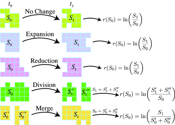
Use of the CCA permits a systematic study of cluster dynamics. For instance, clusters may expand or contract, merge or split between two considered times as illustrated in Fig. 2. We quantify these processes by measuring the probability distribution of the temporal changes in the clusters for the data of GB. We find that when the cell size is 2.2km-by-2.2km, 84% of the clusters evolve from 1981 to 1991 following the three first cases presented in Fig. 2 (no change, expansion or reduction), 6% of the clusters merge from two clusters into one in 1991, and 3% of the clusters split into two clusters.
Next, we apply the CCA to study the dynamics of population growth by investigating Gibrat’s law, which postulates that the mean and standard deviation of growth rates are constant Eeckhout04 ; Gabaix99 ; Ioa03 ; Gab03 ; Eaton97 . The conventional method Gabaix99 ; Ioa03 ; Gab03 is to assume that the populations of a given city or cluster , at times and , are related by
| (1) |
where and are the initial and final populations of cluster , respectively, and is the positive growth factor which varies from cluster to cluster. Following the literature in population dynamics Gabaix99 ; Ioa03 ; Gab03 ; Eeckhout04 , we define the population growth rate of a cluster as , and study the dependence of the mean value of the growth rate, , and the standard deviation, , on the initial population, . The averages and are calculated applying nonparametric techniques hardle ; Silverman86 (see Section IV.2 for details). To obtain the population growth rate of clusters we take into account that not all clusters occupy the same area between and according to the cases discussed in Fig. 2. The figure shows how to calculate the growth rate in each case.
We analyze the population growth in the USA from to ESRI . We apply the CCA to identify the clusters in the data of 1990 and calculate their growth rates by comparing them to the population of the same clusters in 2000 when the data are gridded with a cell size of 2000m by 2000m. We calculate the annual growth rates by dividing by the time interval .
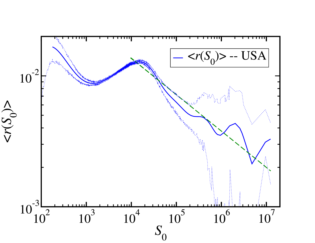
Figure 3A shows a nonparametric regression with bootstrapped 95% confidence bands hardle ; Silverman86 of the growth rate of the USA, (see Section IV.2 for details). We find that the growth rate diminishes from (error includes the confidence bands) for populations below inhabitants to for the largest populations around . We may argue that the mean growth rate deviates from Gibrat’s law beyond the confidence bands. While it is difficult to fit the data to a single function for the entire range, the data show a decrease with approximately following a power-law in the tail for populations larger than . An attempt to fit the data with a power-law yields the following scaling in the tail:
| (2) |
where is the mean growth exponent, that takes a value from Ordinary Least Squares (OLS) analysis montgomery (see Section IV.2 for details on OLS and on the estimation of the exponent error).
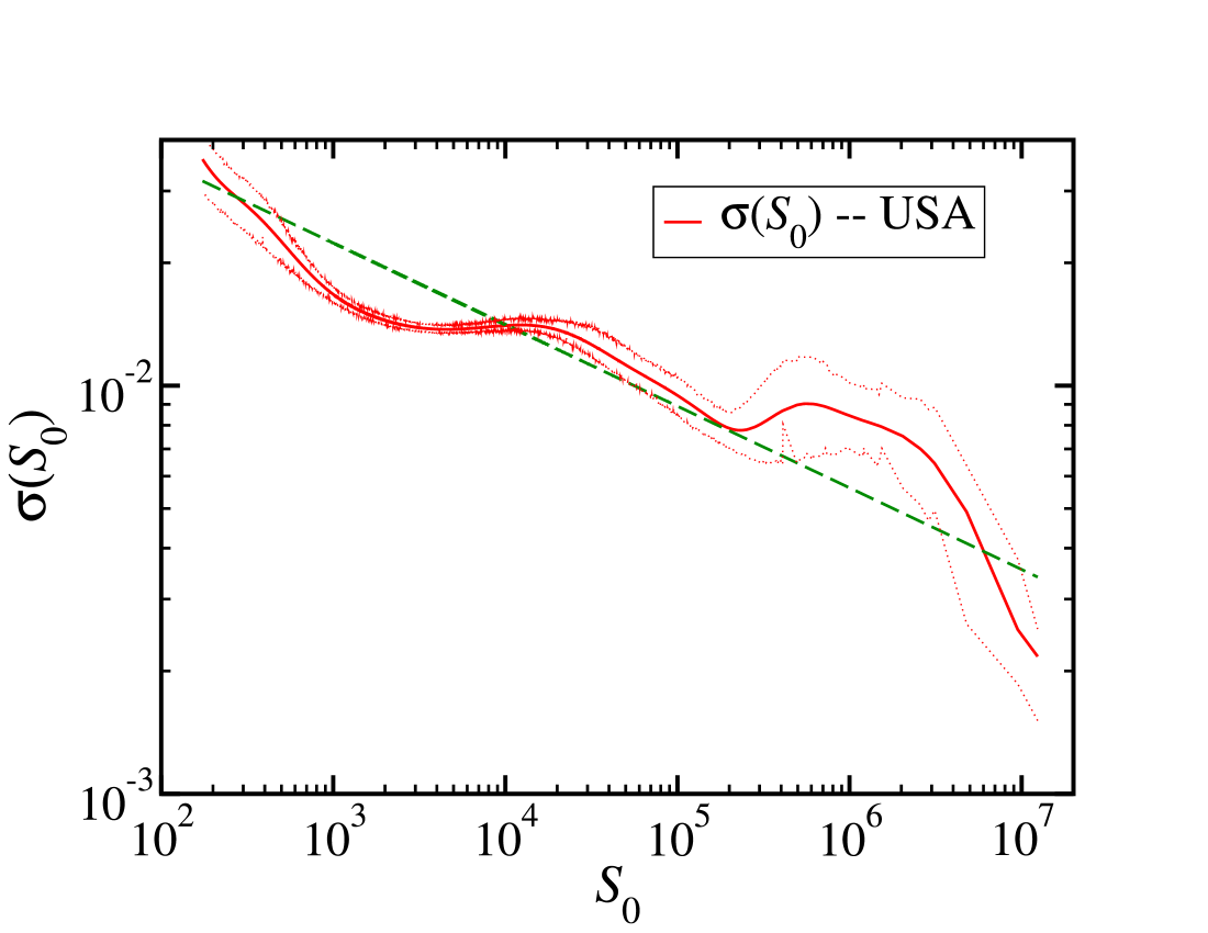
Figure 3B shows the dependence of the standard deviation on the initial population . On average, fluctuations in the growth rate of large cities are smaller than for small cities in contrast to Gibrat’s law. This result can be approximated over many orders of magnitude by the power-law,
| (3) |
where is the standard deviation exponent. We carry out an OLS regression analysis and find that . The presence of a power-law implies that fluctuations in the growth process are statistically self-similar at different scales, for populations ranging from 1000 to 10 million according to Fig. 3B.
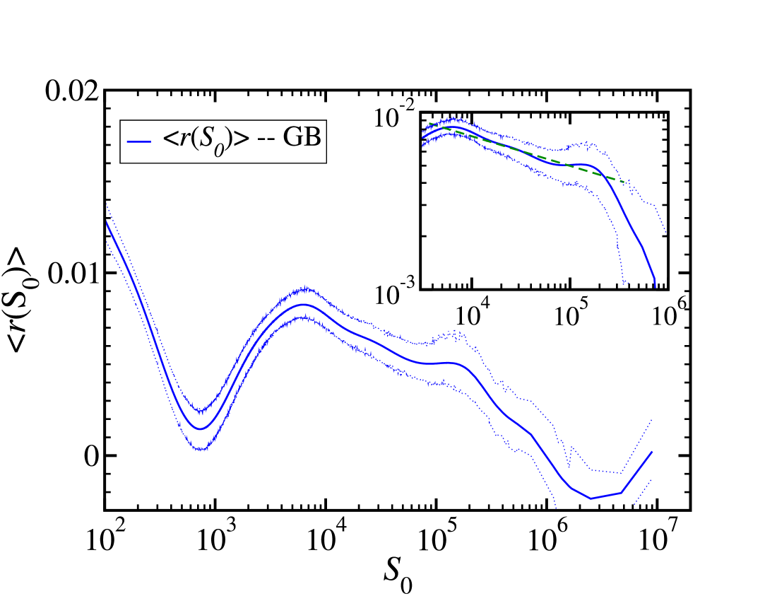
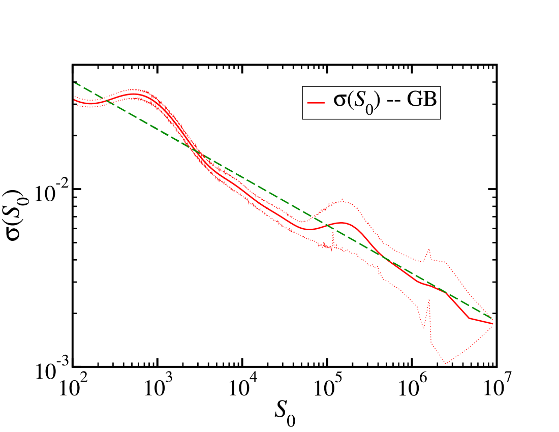
Figure 4 shows the analysis of the growth rate of the population clusters of GB from gridded databases Census with a cell size of 2.2km-by-2.2km at and . The average growth rate depicted in Fig. 4A comprises large fluctuations as a function of , especially for smaller populations. However, a slight decrease with population seems evident from rates around with dropping to zero or even negative values for the largest populations, . We find that 3556 clusters with population around exhibit negative growth rates as well. Thus, the mean rates are plotted on a semi-logarithmic scale in Fig. 4A. When considering intermediate populations ranging from to , the data seem to be following approximately a power-law with from OLS regression analysis, as shown in the inset of Fig. 4A. Figure 4B shows the standard deviation for GB, , exhibiting deviations from Gibrat’s law having a tendency to decrease with population according to Eq. (3) and a standard deviation exponent, , obtained with OLS technique.
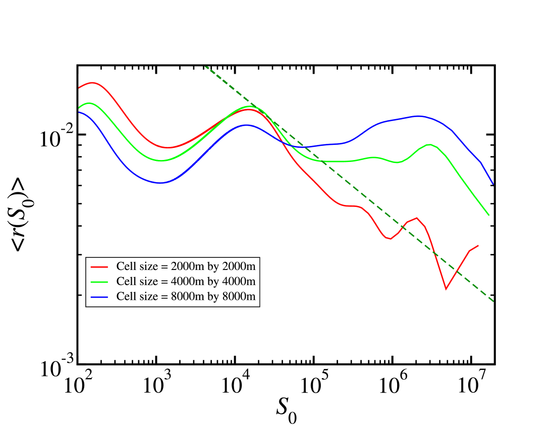
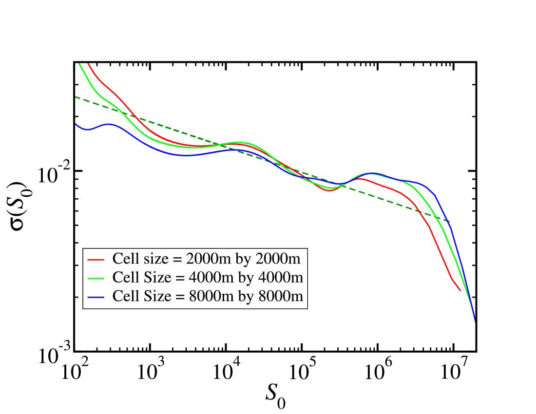
The CCA allows for a study of the growth rates as a function of the scale of observation, by changing the size of the grid. We find (SI Section II.) that the data for GB are approximately invariant under coarse-graining the grid at different levels for both the mean and standard deviation. When the data of the USA are aggregated spatially from cell size 2000m to 8000m, the scaling of the mean rates crosses-over to a flat behavior closer to Gibrat’s law. At the scale of 8000m the mean is approximately constant (with fluctuations). However, we find that, at this scale, all cities in the northeastern the USA spanning from Boston to Washington D.C. form a single cluster. Despite these differences, the scaling of the standard deviation for the USA holds approximately invariant even up to the large scale of observation of 8000m.
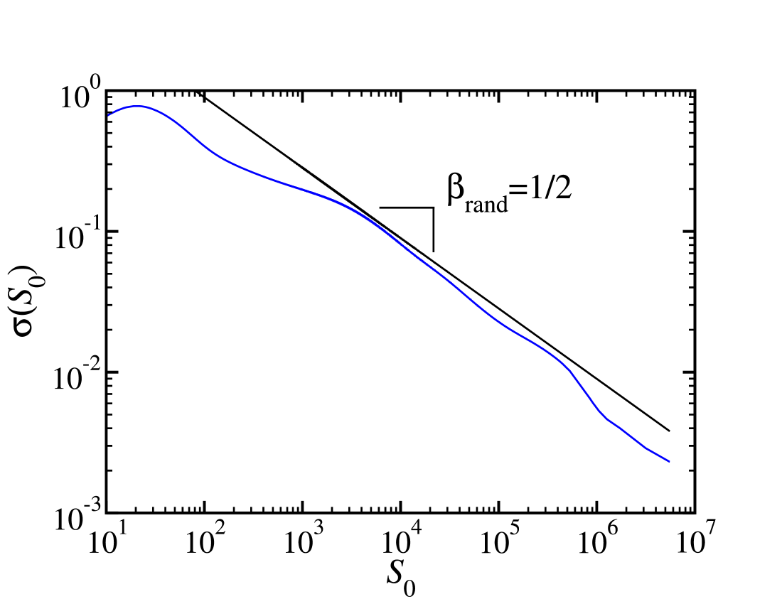
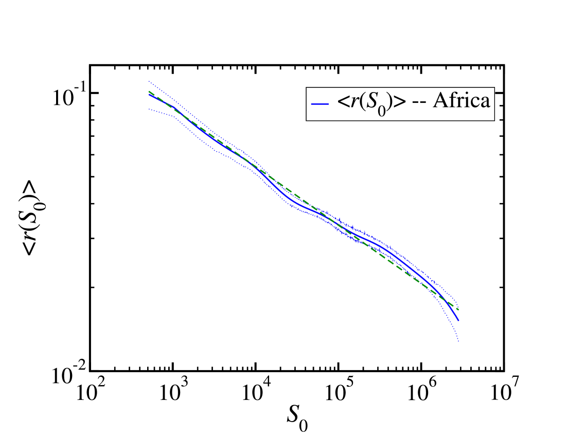
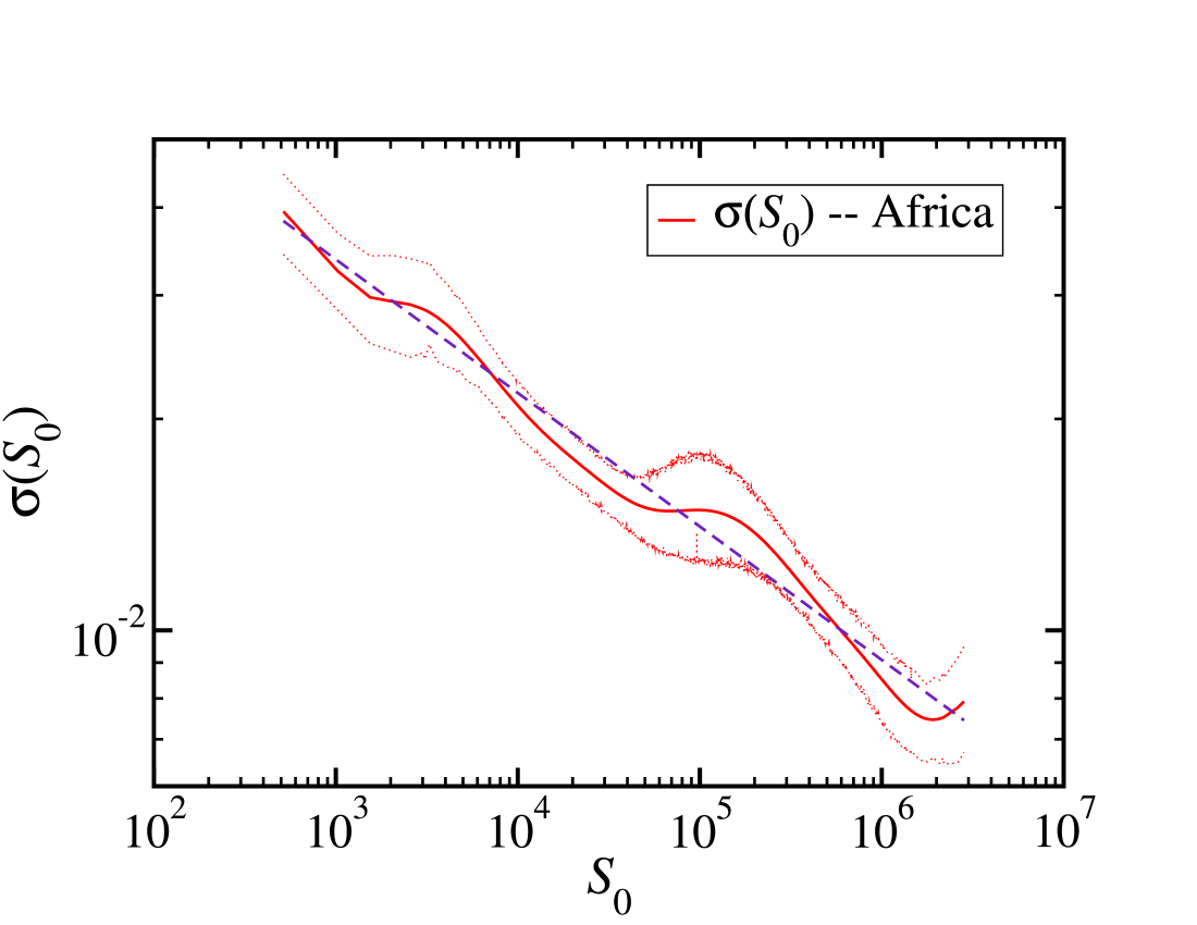
Next, we analyze the population growth in Africa during the period 1960 to 1990 UNESCO . In this case the population data are based on a larger cell size, so we evaluate the data cell by cell (without the application of the CCA). Despite the differences in the economic and urban development of Africa, Great Britain and the USA, we find that the mean and standard deviation of the growth rate in Africa display similar scaling as found for the USA and GB. In Fig. 5A we show the results for the growth rate in Africa when the grid is coarse-grained with a cell size of 77km-by-77km. We find a decrease of the growth rate from to between populations and , respectively. All populations have positive growth rates. A log-log plot of the mean rates shown in Fig. 5A reveals a power-law scaling , with from OLS regression analysis. The standard deviation (Fig. 5B) satisfies Eq. (3) with a standard deviation exponent . The CCA allows for a study of the origin of the observed behavior of the growth rates by examining the dynamics and spatial correlations of the population of cells. To this end, we first generate a surrogate dataset that consists of shuffling two randomly chosen populated cells, and , at time . This swapping process preserves the probability distribution of , but destroys any spatial correlations among the population cells. Figure 4C shows the results of the randomization of the GB dataset, indicating power-law scaling in the tail of with standard deviation exponent . This result can be interpreted in terms of the uncorrelated nature of the randomized dataset (SI Section III). We consider that the population of each cell increases by a random amount with mean value and variance , and that , then . Therefore, the population of a cluster at time can be written as
| (4) |
It can be shown that (SI Section III.):
| (5) |
Randomly shuffling population cells destroys the correlations, leading to (where is the Kronecker delta function) which implies Stanley96 (see SI Section III.).
The fact that lies below the random exponent () for all the analyzed data suggests that the dynamics of the population cells display spatial correlations, which are eliminated in the random surrogate data. The cells are not occupied randomly but spatial correlations arise, since when the population in one cell increases, the probability of growth in an adjacent cell also increases. That is, development attracts further development, an idea that has been used to model the spatial distribution of urban patterns Makse95 . Indeed this ideas are related to the study of the origin of power-laws in complex systems barabasi ; doyle .
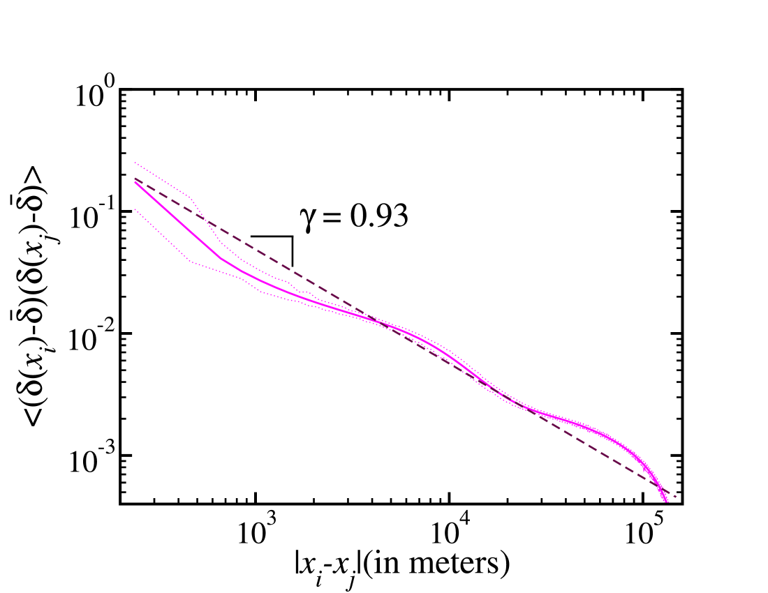
When we analyze the populated cells, we indeed find that spatial correlations in the incremental population of the cells, , are asymptotically of a scale-invariant form characterized by a correlation exponent ,
| (6) |
where is the location of cell . For GB we find (see Fig. 4D). In SI Section III. we show that power-law correlations in the fluctuations at the cell level, Eq. (6), lead to a standard deviation exponent . For , the dimension of the substrate, we recover (larger values of result in the same since when correlations become irrelevant). If , the standard deviation of the populations growth rates has no dependence on the population size (), as stated by Gibrat’s law, stating that the standard deviation does not depend in the cluster size. In the case of GB, gives approximately consistent with the measured value , within the error bars. This observation suggests that the underlying demographic process leading to the scaling in the standard deviation can be modeled as arising from the long-range correlated growth of population cells.
III Discussion
Our results suggest the existence of scale-invariant growth mechanisms acting at different geographical scales. Furthermore, Eq. (3) is similar to what is found for the growth of firms and other macroeconomic indicators Stanley96 ; rossi1 . Thus, our results support the existence of an underlying link between the fluctuation dynamics of population growth and various economic indicators, implying considerable unevenness in economic development in different population sizes. City growth is driven by many processes of which population growth and migration is only one. Our study captures only the growth of population but not economic growth per se. Many cities grow economically while losing population and thus the processes we imply are those that influence a changing population. Our assumption is that population change is an indicator of city growth or decline and therefore we have based our studies on population clustering techniques. Alternatively, the MSAs provides a set of rules that try to capture the idea of city as a functional economic region.
The results we obtain show scale-invariant properties which we have modelled using long-range spatial correlations between the population of cells. That is, strong development in an area attracts more development in its neighborhood and much beyond. A key finding is that small places exhibit larger fluctuations than large places. The implications for locating activity in different places are that there is a greater probability of larger growth in small places, but also a greater probability of larger decline. Opportunity must be weighed against the risk of failure.
One may take these ideas to a higher level of abstraction to study cell-to-cell flows (migration, commuting, etc.) gridded at different levels. As a consequence one may define population clusters, or MSAs, in terms of functional linkages between neighboring cells. In addition one may relax some conditions imposed in the CCA. Here we consider a cell to be part of a cluster only if its population is strictly greater than 0. In SI Section V we relax this condition and study the robustness of the CCA when cells of a higher population than 0 (for instance, 5 and 20) are allowed into clusters and find that even though small clusters present a slight deviation, the overall behavior of the growth rate and standard deviation is conserved.
IV Materials and Methods
IV.1 Information on the datasets
The datasets analyzed in this paper were obtained from the websites http://census.ac.uk, http://www.esri.com/, and http://na.unep.net/datasets/datalist.php, for GB, USA and Africa, respectively, and can be downloaded from http://lev.ccny.cuny.edu/hmakse/cities/city_data.zip.
The datasets consist of a list of populations at specific coordinates at two time steps and . A graphical representation of the data can be seen in Fig. 1C for GB where each point represents a data point directly extracted from the dataset.
To perform the CCA at different scales we coarse-grain the datasets. For this purpose, we overlay a grid on the corresponding map (USA, GB, or Africa) with the desired cell size (for example, 2km-by-2km or 4km-by-4km for the USA). Then, the population of each cell is calculated as the sum of the populations of points (obtained from the original dataset) that fall into this cell.
Table 1 shows information on the datasets and results on USA, GB and Africa for the cell size used in the main text as well as some of the exponents obtained in our analysis.
| Data | Number | Average | Cell Size | Number of | ||||
| of cells | growth rate | clusters | ||||||
| USA | 1.86 mill | 1990 | 2000 | 0.9% | 2km-by-2km | 30,210 | 0.28 0.08 | 0.20 0.06 |
| GB | 0.10 mill | 1981 | 1991 | 0.3% | 2.2km-by-2.2km | 10,178 | 0.17 0.05 | 0.27 0.04 |
| Africa | 2,216 | 1960 | 1990 | 4% | 77km-by-77km | 3,988 | 0.21 0.05 | 0.19 0.04 |
IV.2 Calculation of and and methodology
The average growth rate, , and the standard deviation, , are defined as follows. If we call the conditional probability distribution of finding a cluster with growth rate with the condition of initial population , then we can obtain and through,
| (7) |
and
| (8) |
Once and are calculated for each cluster, we perform a nonparametric regression analysis hardle ; Silverman86 , a technique broadly used in the literature of population dynamics. The idea is to provide an estimate for the relationship between the growth rate and and between the standard deviation and . Following the methods explained in Ref. Silverman86 we apply the Nadaraya-Watson method to calculate an estimate for the growth rate, , with,
| (9) |
and an estimate for the standard deviation with,
| (10) |
where is the population of cluster at time (as defined in the main text), is the growth rate of cluster and is a gaussian kernel of the form,
| (11) |
Finally, we compute the 95% confidence bands (calculated from 500 random samples with replacement) to estimate the amount of statistical error in our results hardle . The bootstrapping technique was applied by sampling as many data points as the number of clusters and performing the nonparametric regression on the sampled data. By performing 500 realizations of the bootstrapping algorithm and extracting the so called ( is not related to the growth rate exponent) quantile we obtain the 95% confidence bands.
To obtain the exponents and of the power-law scalings for and , respectively, we perform an OLS regression analysis montgomery . More specifically, to obtain the exponent from Eq. (3), we first linearize the data by considering the logarithm of the independent and dependent variables so that Eq. (3) becomes . Then, we apply a linear Ordinary Least Square regression that leads to the exponent
| (12) |
where is the number of clusters found using the CCA. Analogously, we obtain the exponent by linearizing and calculating
| (13) |
Next we compute the 95% confidence interval for the exponents and . For this we follow the book of Montgomery and Peck montgomery . The 95% confidence interval for is given by,
| (14) |
where is the t-distribution with parameters and and is the standard error of the exponent defined as
| (15) |
where is the residual and is the variance of .
Finally, we express the value of the exponent in terms of the 95% confidence intervals as,
| (16) |
Acknowledgments
We thank L.H. Dobkins and J. Eeckhout for providing data on MSA and C. Briscoe for help with the manuscript. This work is supported by the National Science Foundation through grant NSF-HSD. J.S.A. thanks the Brazilian agencies CNPq, CAPES, FUNCAP and FINEP for financial support.
References
- (1) Gabaix X (1999) Zipf’s law for cities: an explanation. Quart. J. Econ. 114: 739-767.
- (2) Gabaix X, Ioannides Y M (2003) The evolution of city size distributions, in Handbook of Urban and Regional Economics, Vol.4, eds Henderson J V, Thisse J F (Elsevier Science, Amsterdam), pp 2341-2378.
- (3) Unwin D J (1996) GIS, spatial analysis and spatial statistics. Progress in Human Geography 20:540-551.
- (4) King G, Rosen O, Tanner M A (2004) eds, Ecological Inference: New Methodological Strategies (Cambridge University Press, New York).
- (5) Eeckhout J (2004) Gibrat’s law for (all) cities. Amer. Econ. Rev. 94: 1429-1451.
- (6) Dobkins L H, Ioannides Y M (2000) Spatial interactions among U.S. cities: 1900-1990. Reg. Sci. Urban Econ. 31: 701-731.
- (7) Ioannides Y M, Overman H G (2003) Zipf’s law for cities: an empirical examination Reg. Sci. Urban Econ. 33: 127-137.
- (8) The 1981 and 1991 population census, Crown Copyright, ESRC purchase, http://census.ac.uk/
- (9) ESRI Inc (2000) ArcView 3.2 data sets: North America, Environmental Systems Research Institute, Redlands, CA.
- (10) UNESCO (1987) through GRID, http://na.unep.net/datasets/datalist.php
- (11) Stauffer D (1984) Introduction to percolation theory (Taylor & Francis, London).
- (12) Eaton J, Eckstein Z (1997) Cities and growth: theory and evidence from France and Japan. Reg. Sci. Urban Econ. 27: 443-474.
- (13) Hrdle W (1990) Applied Nonparametric Regression (Cambridge University Press, Cambridge).
- (14) Silverman, B W (1986) Density Estimation for Statistics and Data Analysis (Chapman and Hall, New York).
- (15) Montogomery D C, Peck E A (1992) Introduction to linear regression analysis (John Wiley & Sons, Inc.).
- (16) Stanley M H R et al. (1996) Scaling behavior in the growth of companies. Nature 379: 804-806.
- (17) Makse H A, Havlin S, Stanley H E (1995) Modelling urban growth patterns. Nature 377: 608-612.
- (18) Barabási A-L, Albert R (1999) Emergence of scaling in random networks. Science, 286, 509-512.
- (19) Carlson J M, Doyle J (2002) Complexity and robustness. PNAS, 99:2538-2545.
- (20) Rossi-Hansberg E, Wright M L J (2007) Establishment size dynamics in the aggregate economy. Amer. Econ. Rev. 97: 1639-1666.
A 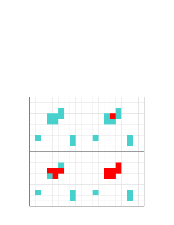
B ![[Uncaptioned image]](/html/0808.2202/assets/x2.png)
Fig. 1
C ![[Uncaptioned image]](/html/0808.2202/assets/x3.png)
Fig. 1
A
 B
B
A
 B
B
 C
C
 D
D
A
 B
B
SUPPORTING INFORMATION
Laws of Population Growth
Hernán D. Rozenfeld, Diego Rybski, José S. Andrade Jr.,
Michael Batty, H. Eugene Stanley, and Hernán A. Makse
As supplementary materials we provide the following: In Section V we present tables with details on our results using the CCA and results presented in previous papers to allow for comparison between the different approaches. In Section VI we study the stability of the scaling found in the text under a change of scale in the cell size. In Section VII we detail the calculations to relate spatial correlations between the population growth and namely the relation . In Section VIII we describe the random surrogate dataset used to further test our results. In Section IX we further test the robustness of the CCA by proposing a small variation in the algorithm.
V Clusters at different scales and comparison with Metropolitan Statistical Areas
In this section, Tables S1 and S2 allow for a detailed comparison of urban clusters obtained with the CCA applied to the USA in 1990, and the populations of MSA from US Census Bureau used in previous studies of population growth dobkins00 ; Ioa03 ; Eeckhout04 .
We can see that the MSA presented by Eeckhout (2004) typically correspond to our clusters using cell sizes of 4km and 8km. For example, for the New York City region Eeckhout’s data are well approximated by a cell size of 4km, but Los Angeles is better approximated when using a cell size of 8km. On the other hand Dobkins-Ioannides (2000) data are better described by cell sizes of 2km or 4km. For instance, Chicago is well described by a cell size of 4km and Los Angeles is better described by a cell size of 2km.
An interesting remark is that the population of Los Angeles when using cell sizes of 2km, 4km and 8km does not vary as much as that for New York. This could be caused by the fact that major cities in the northeast of USA are closer to each other than large cities in the southwest, which may be attributed to land or geographical constraints.
It is important relate the results of Table S2 with an ecological fallacy. As the cell size is increased, the population of a cluster also increases, as expected, because the cluster now covers a larger area. This is not a direct manifestation of an ecological fallacy which, would appear if the statistical results (growth rate vs. S or standard deviation vs. S) gave different results as the cell size increases. In Fig. 1 and Fig. 2 in the SI Section VI, we observe that the growth rate and standard deviation for the USA and GB follow the same form, except for the case of the growth rate in the USA in which different cell sizes show deviations from each other. The later may be an indicative of an ecological fallacy. In this case, it is not obvious what cell size is the “correct” one. We consider this point (the possibility to choose the cell size) to be a feature of the CCA, since one may appropriately pick the cell size according to the specific problem one is studying.
Table S1: Top 10 largest MSA of the USA in 1990 from previous analysis of population growth
| Dobkins - Ioannides | Eeckhout | |||
| MSA | Population | MSA | Population | |
| 1 | NYC NY206 | 9,372,000 | NYC-North NJ-Long Is., NY-NJ-CT-PA | 19,549,649 |
| 2 | Los Angeles CA172 | 8,863,000 | Los Angeles-Riverside-Orange County, CA | 14,531,529 |
| 3 | Chicago IL59 | 7,333,000 | Chicago-Gary-Kenosha, IL-IN-WI | 8,239,820 |
| 4 | Philadelphia PA228 | 4,857,000 | Washington-Baltimore, DC-MD-VA-WV | 6,727,050 |
| 5 | Detroit MI80 | 4,382,000 | San Francisco-Oakland-San Jose, CA | 6,253,311 |
| 6 | Washington DC312 | 3,924,000 | Philadelphia-Wilmington-Atlantic City | 5,892,937 |
| PA-NJ-DE-MD | ||||
| 7 | San Francisco CA266 | 3,687,000 | Boston-Worcester-Lawrence, MA-NH-ME-CT | 5,455,403 |
| 8 | Houston TX129 | 3,494,000 | Detroit-Ann Arbor-Flint, MI | 5,187,171 |
| 9 | Atlanta GA19 | 2,834,000 | Dallas-Fort Worth, TX | 4,037,282 |
| 10 | Boston MA39 | 2,800,000 | Houston-Galveston-Brazoria, TX | 3,731,131 |
Table S2: Top 10 largest clusters of the USA in 1990 from our analysis for different cell sizes. The city names are the major cities that belong to the clusters and were picked to show the areal extension of the cluster.
| Cell = 1km | Cell = 2km | Cell = 4km | Cell = 8km | |||||
| Cluster | Population | Cluster | Population | Cluster | Population | Cluster | Population | |
| 1 | NYC | 7,012,989 | NYC-Long Is. | 12,511,237 | NYC-Long Is. | 17,064,816 | NYC-Long Is. | 41,817,858 |
| Newark | N. NJ-Newark | North NJ | ||||||
| Jersey City | Jersey City | Philadelphia | ||||||
| D.C.-Boston | ||||||||
| 2 | Chicago | 2,312,783 | Los Angeles | 9,582,507 | Los Angeles | 10,878,034 | Los Angeles | 13,304,233 |
| Long Beach | Long Beach | San Clemente | ||||||
| Pomona | Riverside | |||||||
| 3 | Los Angeles | 1,411,791 | Chicago | 4,836,529 | Chicago | 7,230,404 | Chicago | 9,288,345 |
| Rockford | Gary | Gary | ||||||
| Rockford | Rockford | |||||||
| Milwaukee | ||||||||
| 4 | Philadelphia | 1,282,834 | Philadelphia | 3,151,704 | Washington | 5,316,890 | San Francisco | 5,736,479 |
| Wilmington | Baltimore | Santa Cruz | ||||||
| Springfield | Brentwood | |||||||
| 5 | Boston | 759,024 | Detroit | 2,906,453 | Philadelphia | 4,935,734 | Detroit | 4,442,723 |
| Trenton | Ann Arbor | |||||||
| Wilmington | Monroe | |||||||
| Sarnia | ||||||||
| 6 | Newark | 581,048 | San Francisco | 2,601,639 | San Francisco | 4,766,960 | Miami | 4,000,432 |
| San Jose | San Jose | Port St. Lucie | ||||||
| Concord | ||||||||
| 7 | San Francisco | 507,300 | Washington | 2,059,421 | Detroit | 3,722,778 | Dallas | 3,536,186 |
| Alexandria | Waterford | Fort Worth | ||||||
| Bethesda | Canton | |||||||
| 8 | Washington | 504,068 | Phoenix | 1,556,077 | Miami | 3,719,773 | Houston | 3,425,647 |
| W. Palm Beach | ||||||||
| 9 | Jersey City | 438,591 | Boston | 1,498,208 | Dallas | 3,134,233 | Cleveland | 3,233,341 |
| Lowell | Fort Worth | Canton | ||||||
| Quincy | ||||||||
| 10 | Baltimore | 437,413 | Miami | 1,465,490 | Boston | 3,064,925 | Pittsburgh | 3,214,661 |
| Brockton | Youngstown | |||||||
| Nashua | Morgantown | |||||||
VI Scaling under coarse-graining
In this section we test the sensitivity of our results to a coarse-graining of the data. We analyze the average growth rate and the standard deviation for GB and the USA by coarse-graining the data sets at different levels.
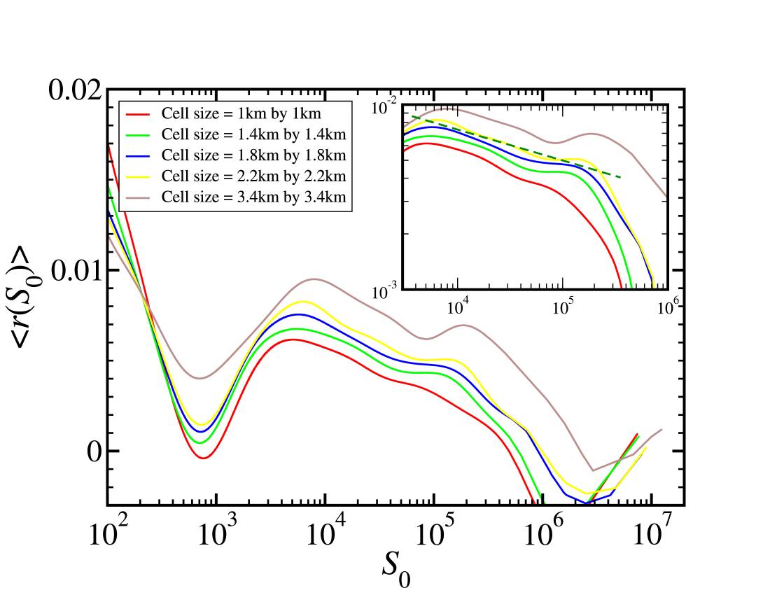
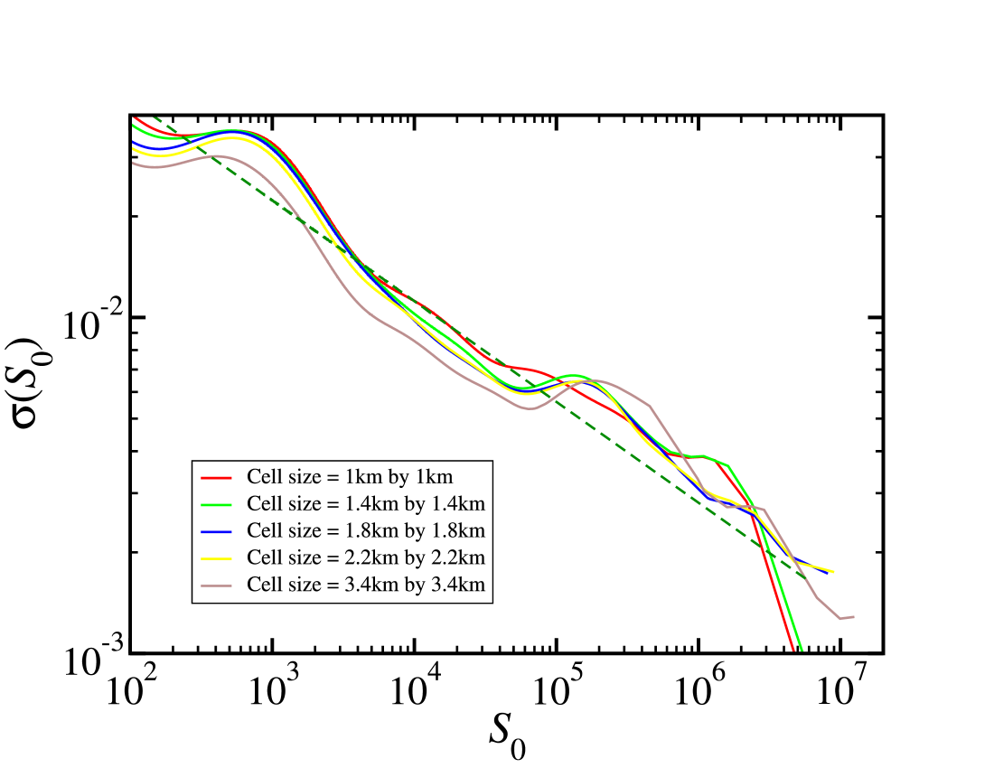
In Fig. 6A we observe that although the results are not identical for all coarse-grainings, they are statistically similar, showing a slight decay in the growth rate. Moreover, we see that cities of size and still exhibit a tendency to have negative growth rates for all levels of coarse-graining, as explained in the main text. In the case of the USA (Fig. 7A) there is a crossover to a flat behavior at a cell size of 8000m, although at this scale all the northeast USA becomes a large cluster of 41 million inhabitants. On the other hand, Figs. 6B, 7B show that the scaling of Eq. (3) in the main text, , still holds when using the coarse-grained datasets on both GB and the USA.
A
 B
B
A
 B
B
VII Correlations
In this section we elaborate on the calculations leading to the relation between Gibrat’s law and the spatial correlations in the cell population. We first show that when the population cells are randomly shuffled (destroying any spatial correlations between the growth rates of the cells), the standard deviation of the growth rate becomes , where Stanley96 . Then, we show that long-range spatial correlations in the population of the cells leads to the relation as stated at the end of Section II in the main text.
Assuming that the population growth rate is small (), we can write . Replacing in Eq. (1) in the main text we obtain
| (17) |
We define the standard deviation of the populations as , which is a function of :
| (18) |
This quantity is easier to relate to the spatial correlations of the cells than the standard deviation of the growth rates . Then, since and , we obtain,
| (19) |
where as defined in the main text. Therefore, using Eq. (3) in the main text,
| (20) |
As stated in the main text, the total population of a cluster at time is the sum of the populations of each cell, , where is the number of cells in cluster . The population of a cluster at time can be written as
| (21) |
where is the increment in the population of cell from time to (notice that can be negative). Therefore, the standard deviation is
| (22) |
After the process of randomization explained in Section II main text, the correlations between the increment of population in each cell are destroyed. Thus,
| (23) |
where . Replacing in Eq. (22) and since , we obtain
| (24) |
Comparing with Eq. (20) we obtain for this uncorrelated case.
Let us assume that the correlation of the population increments , decays as a power-law of the distance between cells indicating long-range scale-free correlations. Thus, asymptotically
| (25) |
where denotes the position of the cell and is the correlation exponent (for , the correlations tend to a constant). For large clusters, we can approximate the double sum in Eq. (22) by an integral. Then, assuming that the shape of the clusters can be approximated by disks of radius , for we obtain
| (26) |
where is the area of each cell and the radius of the cluster. Since , we finally obtain,
| (27) |
Using and Eq. (20) we arrive at,
| (28) |
Equation (28) shows that Gibrat’s Law is recovered when the correlation of the population increments is a constant, independent from the positions of the cells; that is when all the populations cells are increased equally. In other words, if , the standard deviation of the populations growth rates has no dependence on the population size (), as stated by Gibrat’s law. The random case is obtained for , where is the dimensionality of the substrate. In this case and . For , the correlations become irrelevant and we still find the uncorrelated case . For intermediate values we obtain .
VIII Random surrogate dataset
In this section we elaborate on the randomization procedure used to understand the role of correlations in population growth.
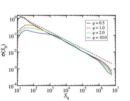
Figure 4C in the main text shows the standard deviation when the population of each cluster is randomized, breaking any spatial correlation in population growth. For clusters with a large population, follows a power-law with exponent , and for small , presents deviations from the power-law function as seen in Fig. 4C with smaller standard deviation than the prediction of the random case. This deviation is caused by the fact that the population of a cluster is bound to be positive: a cluster with a small population cannot decrease its population by a large number, since it would lead to negative values of . This produces an upper bound in fluctuations of the growth rate for small and results in smaller values of than expected (below the scaling with exponent ).
To support this argument, we carry out simulations using the clusters of GB, where the population of each cell is replaced with random numbers following an exponential distribution with probability . The decay-constant, , is extracted from the data of GB to mimic the original distribution. This is done through a direct measure of from the GB dataset and fitting the data using OLS regression analysis. We obtain the population of cell at time by picking random numbers for the population increments following a uniform distribution in the range . Here determines the variance of the increments. Since the population cannot be negative we impose the additional condition . Figure 8 shows the results of the standard deviation for four different -values for this uncorrelated model. We find that the tail of reproduces the uncorrelated exponent . For small we find that the standard deviation levels off to an approximately constant value as in the surrogate data of Fig 4C. The crossover from an approximately constant to a power-law moves to smaller values of the population as the standard deviation in the is smaller (smaller value of ). Such behavior can be understood since the condition imposes a lower “wall” in the random walk specified by . As the initial population gets smaller, the walker “feels” the presence of the wall and the fluctuations decrease accordingly, thus explaining the deviations from the power-law with exponent for small population values. Therefore, as the value of decreases, the small population plateau disappears as observed in Fig. 8.
IX A variation of the CCA
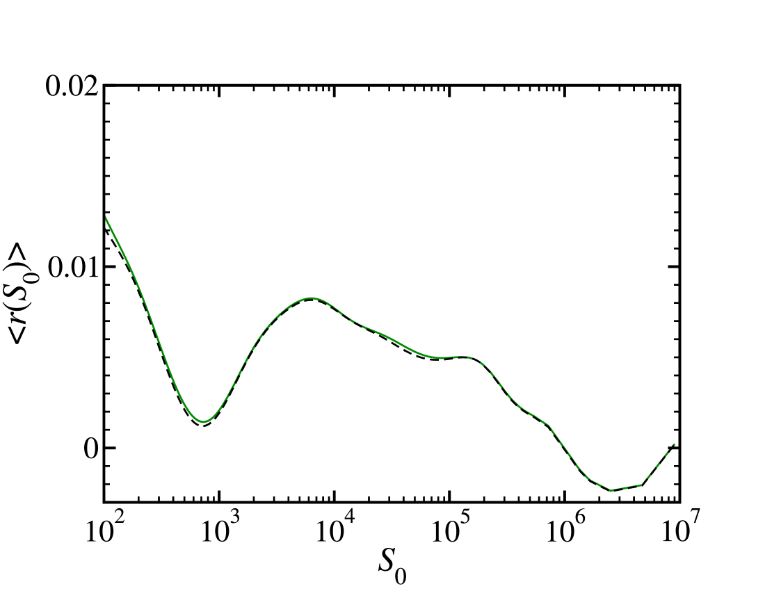
In this section we study a variation of the CCA. In the main text we stop growing a cluster when the population of all boundary cells have unpopulated, that is, have population exactly 0. In other words, clusters are composed by cell with population strictly greater than 0. It is important to analyze whether this stopping criteria can be relaxed to including cell which have a population larger that a given threshold. In Fig. 9A and Fig. 9B we show the results for the population growth rate and standard deviation, respectively, in GB when the cell size is 2.2km-by-2.2km (as in the main text) but including cells with a population strictly larger than 5 and 20.
A
 B
B
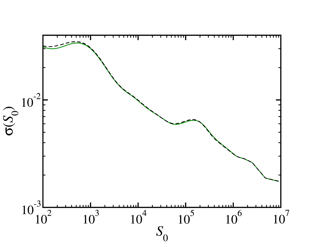
Although for small population clusters we observe a slight variation in the growth rate and in the standard deviation, the results show that the thresholds do not influence the global statistics when compared to the plots in the main text.