Jamming I: A volume function for jammed matter

Abstract

We introduce a “Hamiltonian”-like function, called the volume function, indispensable to describe the ensemble of jammed matter such as granular materials and emulsions from a geometrical point of view. The volume function represents the available volume of each particle in the jammed systems. At the microscopic level, we show that the volume function is the Voronoi volume associated to each particle and in turn we provide an analytical formula for the Voronoi volume in terms of the contact network, valid for any dimension. We then develop a statistical theory for the probability distribution of the volumes in 3d to calculate an average volume function coarse-grained at a mesoscopic level. The salient result is the discovery of a mesoscopic volume function inversely proportional to the coordination number. Our analysis is the first step toward the calculation of macroscopic observables and equations of state using the statistical mechanics of jammed matter, when supplemented by the condition of mechanical equilibrium of jamming that properly defines jammed matter at the ensemble level.

1 Introduction

The development of a statistical mechanics for granular matter and other jammed materials presents many difficulties. First, the macroscopic size of the constitutive particles forbids equilibrium thermalization of the system. Second, the fact that energy is constantly dissipated via frictional interparticle forces further renders the problem outside the realm of equilibrium statistical mechanics. In the absence of energy conservation laws, a new statistical approach is needed in order to describe the system properties. Along this line of research, Edwards [1] has proposed to replace the energy by the volume as the conservative quantity of the system. Then a canonical partition function of jammed states can be defined and a statistical mechanical analysis ensues.

While it is always possible to measure the total volume of the system, it is unclear how to treat the volume fluctuations at the microscopic level. Thus, it is still an open problem the definition of an analogous “Hamiltonian” that describes the microstates of jammed matter. Such a “Hamiltonian” is called the volume function [1], denoted ${\cal W}$. The idea is to partition the granular material into $N$ elements and associate an additive volume function to them, ${\cal W}_{i}$, such that the total system volume, ${\cal W}$, is

$${\cal W}=\sum_{i=1}^{N}{\cal W}_{i}.$$ (1)

From a theoretical perspective, initial attempts to define the volume function involved modelling under mean-field approximations proposed by Edwards [1] not taking into account the contact network. The necessary definition in terms of the internal degrees of freedom has been pursued by Ball and Blumenfeld [2, 3] who have shown by an exact triangulation method that the volume defining each grain can be given in terms of the contact points using vectors constructed from them. The method consists of defining shortest loops of grains in contact with one another, thus defining the void space around a central grain.

A simpler version for the volume function was also given by Edwards as the area in 2d or volume in 3d encompassing the first coordination shell of the grains in contact [4]. The resulting volume is the antisymmetric part of the fabric tensor, the significance of which is its appearance in the calculation of stress transmission through granular packings [2]. This definition is only an approximation of the space available to each grain since there is an overlap of volumes for grains belonging to the same coordination shell. Thus, it overestimates the total volume of the system: $\sum{\cal W}_{i}>{\cal W}$ [4].

Furthermore, both definitions of ${\cal W}_{i}$ in [2, 3, 4] are proportional to the coordination number of the grain. This is in contrast to expectation since the free volume available to a grain should decrease as the number of contacts increase. Indeed, this observation is corroborated by experimental studies of jammed granular matter using X-ray tomography [5] to determine the volume per grain versus coordination number.

Based on the idea that the volume function represents a free volume available per grain, we introduce a new “Hamiltonian” to describe the microstates of jammed matter. We analytically calculate the volume function and demonstrate that it is equal to the Voronoi volume associated to each particle, partitioning the space into a set of regions, associating all grain centroids in each region to the closest grain centroid. Even though the Voronoi construction successfully tiles the system, its drawback in its use as a volume function was that, so far, there was no analytical formula to calculate it. Our approach provides this formula in terms of the contact network. Furthermore we introduce a theory of volume fluctuations to calculate a coarse-grained average volume function defined at the mesoscopic level that reduces the degrees of freedom to only the coordination number $z$. We find that the volume function is inversely proportional to $z$ in agreement with the tomography experiments of [5]. Our analysis also provides an equation of state, relating volume with coordination number in the limit of fully random system. Indeed, it predicts with good accuracy the limiting cases of random loose and random close packing fractions. Our results allow construction of a statistical partition function from which macroscopic observables can be calculated. This case is treated in more detail in the second part of this work: Jamming II [6].

1.1 Outline

This paper is the first installment in a series of papers devoted to different aspects of jammed matter and is the main theoretical contribution for the subsequent statistical mechanics approach. The present paper is an extended version of the Supplementary Information Section I in [6]. The outline is as follows: Section 2 details the development of the microscopic volume function in terms of the particle coordinates. The relation of this form with the Voronoi volume of each particle is discussed in Section 3. Section 4 discusses the statistical theory to calculate the probability distribution of the Voronoi volumes leading to the average mesoscopic volume function discussed in Section 5. Section 6 tests the assumptions of the theory and we finish with the outlook in Section 7.

2 Microscopic volume function

We start by defining a volume function for rigid spherical grains of equal size in terms of particle positions. The volume function represents the available volume to the particle with the constraint of fixed total system volume. Since we are dealing with rigid jammed particles, the available free volume is in principle zero since the particle by definition cannot move. However, we allow the particle to move by introducing a soft interparticle potential and then taking the limit of particle rigidity to infinity. The resulting volume is well-defined, representing the free volume associated with each grain in the jammed packing.

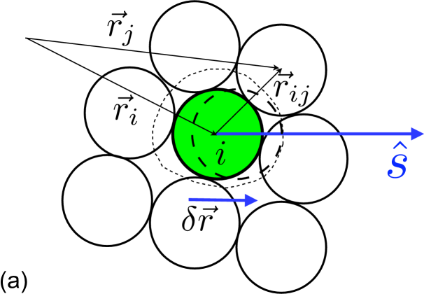
Figure 1: Definition of the volume function. Particle $i$ moves in the direction of $\hat{s}$ as indicated such that the deformation energy is below a threshold $\epsilon$. When averaged over all directions $\hat{s}$, this process defines the available volume under the threshold $\epsilon$ demarcated by the thin dotted line. The volume function is then obtained in the limit of infinite rigidity of the particles, $\alpha\to\infty$.

We consider a rigid particle of radius $R$ jammed at position $\vec{r}_{i}$ in contact with another particle at position $\vec{r}_{j}$ such that $\vec{r}_{ij}=\vec{r}_{j}-\vec{r}_{i}=r_{ij}\hat{r}_{ij}$ (see Fig. 1). In order to calculate the volume associated with such a particle we allow it to move by introducing a generic interparticle soft-potential, $f_{\alpha}$, determined by an exponent $\alpha$ governing the rigidity of the particles (see below). A small energy threshold $\epsilon$ is introduced in order to drive the particle in a certain direction $\hat{s}$ as indicated in Fig. 1. A small displacement $\delta\vec{r}=\delta r\hat{s}$ of particle $i$ along the $\hat{s}$ direction results in an increase of energy $E$ between particles $i$ and its neighbors:

$$E=\sum_{\delta\vec{r}\cdot\vec{r}_{ij}>0}f_{\alpha}(|\vec{r}_{ij}|-|\vec{r}_{ij}+\delta\vec{r}|)\approx\sum_{\hat{s}\cdot\hat{r}_{ij}>0}f_{\alpha}((\hat{s}\cdot\hat{r}_{ij})\delta{r}),$$ (2)

where the sum is taken over all the neighbors of particle $i$. The soft pair potential $f_{\alpha}$ can be any repulsive function provided it approaches the hard sphere limit when the control parameter $\alpha\to\infty$, implying

$$\lim_{\alpha\rightarrow\infty}\frac{f_{\alpha}(x)}{f_{\alpha}(y)}=0,\forall\ x<y.$$ (3)

[A possible function is simply $f_{\alpha}(x)=x^{\alpha}$, the case $\alpha=5/2$ corresponds to the Hertz potential]. This condition implies that

$$\begin{split}\lim_{\alpha\rightarrow\infty}\sum_{i}f_{\alpha}(x_{i})=&f_{\infty}(\max_{i}(x_{i}))\times\lim_{\alpha\rightarrow\infty}\sum_{i}\frac{f_{\alpha}(x_{i})}{f_{\infty}(\max_{i}(x_{i}))}\\ =&f_{\infty}(\max_{i}(x_{i})),\end{split}$$ (4)

and therefore from Eq. (2), we obtain:

$$E=f_{\infty}(\max_{i}(\hat{s}\cdot\hat{r}_{ij})\delta{r}).$$ (5)

We define the available volume to a grain, ${\cal W}_{i}^{\rm a}$, under the energy threshold $\epsilon$ as:

$${\cal W}_{i}^{\rm a}=\int\Theta(\epsilon-E)dV=\oint\int_{0}^{\infty}\Theta(\epsilon-E)\delta{r}^{d-1}d[\delta{r}]ds,$$ (6)

where $d$ is the dimension of the system, $ds$ is an infinitesimal solid angle in $d$ dimensions, and the available volume ${\cal W}_{i}^{\rm a}$ is averaged over all the directions of the $d$ dimensional solid angle.

The integration over $\delta{r}$ can be simplified when $\alpha\rightarrow\infty$ since for a fixed direction $\hat{s}$ we have:

$$\begin{split}\lim_{\alpha\rightarrow\infty}\int_{0}^{\infty}\Theta(\epsilon-E)\delta{r}^{d-1}d[\delta{r}]&\\ =\lim_{\alpha\rightarrow\infty}\int_{0}^{\infty}\Theta[\epsilon-f_{\alpha}(\max_{\hat{s}\cdot\hat{r}_{ij}>0}(\hat{s}\cdot&\hat{r}_{ij})\delta{r})]\delta{r}^{d-1}d[\delta{r}]\\ \propto&\min_{\hat{s}\cdot\hat{r}_{ij}>0}(\hat{s}\cdot\hat{r}_{ij})^{-d}.\end{split}$$ (7)

Thus, we obtain:

$${\cal W}_{i}^{\rm a}\propto\oint\min_{\hat{s}\cdot\hat{r}_{ij}>0}(\hat{s}\cdot\hat{r}_{ij})^{-d}ds.$$ (8)

Equation (8) can be interpreted as follows: for each direction $\hat{s}$, the available volume is determined by the particle position whose projection of the distance to particle $i$ in the $\hat{s}$ direction is minimal. The total volume is then the average over all directions $\hat{s}$. The proportionality constant in Eq. (8) can be determined because ${\cal W}_{i}^{\rm a}$ is equal to the volume of the grains, $V_{g}$, when the coordination number $z\rightarrow\infty$, suggesting that, in this limit, $\min_{\hat{s}\cdot\hat{r}_{ij}>0}(\hat{s}\cdot\hat{r}_{ij})^{-d}=1$ for any $\hat{s}$. That is,

$${\cal W}_{i}^{\rm a}=\frac{V_{g}}{\oint ds}\oint\min_{\hat{s}\cdot\hat{r}_{ij}>0}(\hat{s}\cdot\hat{r}_{ij})^{-d}ds.$$ (9)

For mono-disperse spherical particles, $V_{g}=\frac{R^{d}}{d}\oint ds$. Thus, we have

$$\begin{split}{\cal W}_{i}^{\rm a}=\frac{1}{d}\oint\left(\min_{\hat{s}\cdot\hat{r}_{ij}>0}\frac{R}{\hat{s}\cdot\hat{r}_{ij}}\right)^{d}ds\\ =\frac{1}{d}\oint\left(\min_{\hat{s}\cdot\hat{r}_{ij}>0}\frac{r_{ij}}{2\hat{s}\cdot\hat{r}_{ij}}\right)^{d}ds,\end{split}$$ (10)

where we have replaced $r_{ij}=2R$ for nearest neighbors in the last equation. This allows us to generalize the volume formula to satisfy additivity and relate it to the Voronoi volume as shown below.

Equation (10) is not additive, and is different from the Voronoi volume since only contacting particles are considered in the calculation. Strictly speaking, only at the limit when the coordination number $z\rightarrow\infty$, and all the geometrical constraints come from contacting particles, the volume function Eq. (10) converges to the Voronoi volume. However, the formula becomes additive when considering all particles rather than the nearest neighbors in the calculation of the minimum integrand in Eq. (10). This approach is justified since non-contact particles may contribute to the energy of deformation in Eq. (5). Further, if the minimum in Eq. (10) is taken over all the particles in the packing, ${\cal W}_{i}^{\rm a}$ is exactly equal to the Voronoi volume, which is obviously additive. In turn we provide a formula for the calculation of the Voronoi volume in terms of particle positions, as shown next.

3 A formula for the Voronoi volume

First, we recall the definition of a Voronoi cell as a convex polygon whose interior consists of all points which are closer to a given particle than to any other.

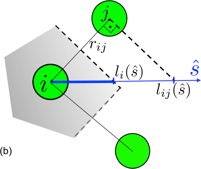
Figure 2: The limit of the Voronoi cell (grey area) of particle $i$ in the direction $\hat{s}$ is $l_{i}(\hat{s})=\min_{j}l_{ij}(\hat{s})/2$, where $l_{ij}=r_{ij}/\cos\theta_{ij}$. Then the Voronoi volume is proportional to the integration of $l_{i}(\hat{s})$ over $\hat{s}$ as in Eq. (14).

Formally, the volume of the Voronoi cell of particle $i$ can be calculated as (see Fig. 2):

$${\cal W}_{i}^{\rm vor}=\oint\int_{0}^{l_{i}(\hat{s})}r^{d-1}drds=\frac{1}{d}\oint l_{i}(\hat{s})^{d}ds,$$ (11)

where $l_{i}(\hat{s})$ is the distance from particle $i$ to the boundary of its Voronoi cell in the $\hat{s}$ direction. Note that this definition is valid whether the particle $j$ is in contact with $i$ or not. If we denote the distance from particle $i$ to any particle $j$ at $\hat{s}$ direction as

$$l_{ij}(\hat{s})\equiv r_{ij}/(\hat{s}\cdot\hat{r}_{ij}),$$ (12)

then $l_{i}(\hat{s})$ is the minimum of $l_{ij}(\hat{s})/2$ over all the particles $j$ for any $l_{ij}(\hat{s})>0$ (see Fig. 2). This leads to

$$l_{i}(\hat{s})=\min_{l_{ij}(\hat{s})>0}l_{ij}(\hat{s})/2=\min_{\hat{s}\cdot\hat{r}_{ij}>0}\frac{r_{ij}}{2\hat{s}\cdot\hat{r}_{ij}}.$$ (13)

Substituting into Eq. (11), we prove that the Voronoi volume is indeed the volume available per particle as calculated in Eq. (10):

$${\cal W}_{i}^{\rm vor}=\frac{1}{d}\oint\left(\min_{\hat{s}\cdot\hat{r}_{ij}>0}(\frac{r_{ij}}{2\hat{s}\cdot\hat{r}_{ij}})\right)^{d}ds={\cal W}_{i}^{\rm a}.$$ (14)

Formula (14) can be rewritten as

$${\cal W}_{i}^{\rm vor}=\frac{1}{\oint ds}\oint{\cal W}_{i}^{s}ds=\langle{\cal W}_{i}^{s}\rangle_{s},$$ (15)

where we define the orientational volume for the $i$ particle in the $\hat{s}$ direction as:

$${\cal W}_{i}^{s}\equiv V_{g}\left(\frac{1}{2R}\min_{\hat{s}\cdot\hat{r}_{ij}>0}\frac{r_{ij}}{\hat{s}\cdot\hat{r}_{ij}}\right)^{d}.$$ (16)

Let us recapitulate and recall the three volumes defined so far which are interrelated: the Voronoi and the available volume which satisfy ${\cal W}_{i}^{\rm vor}={\cal W}_{i}^{\rm a}$, and the orientational volume which satisfies $\langle{\cal W}_{i}^{s}\rangle_{s}={\cal W}_{i}^{\rm vor}$. All the quantities are additive, thus they provide the total volume of the system:

$${\cal W}=\sum_{i}{\cal W}_{i}^{\rm vor}=\sum_{i}{\cal W}_{i}^{\rm a}=\sum_{i}\langle{\cal W}_{i}^{s}\rangle_{s}.$$ (17)

For isotropic packings, ${\cal W}_{i}^{s}$ (without the average over $\hat{s}$) is also additive since the choice of orientation $\hat{s}$ is arbitrary. Thus, we obtain:

$${\cal W}=\sum_{i}\langle{\cal W}_{i}^{s}\rangle_{s}=\langle\sum_{i}{\cal W}_{i}^{s}\rangle_{s}=\sum_{i}{\cal W}_{i}^{s}.$$ (18)

This property reduces the calculations, since there is no need for an orientational average. We define the orientational free volume function as:

$$W={\cal W}_{i}^{s}-V_{g},$$ (19)

and the reduced orientational free volume function

$${w_{i}}^{s}=\frac{{\cal W}_{i}^{s}-V_{g}}{V_{g}},$$

with its average value, $w$, over the particles, $i$, for isotropic systems as:

$$w\equiv\langle w_{i}^{s}\rangle_{i}\equiv\frac{\langle{\cal W}_{i}^{s}\rangle_{i}-V_{g}}{V_{g}}=\left\langle\left(\frac{1}{2R}\min_{\hat{s}\cdot\hat{r}_{ij}>0}\frac{r_{ij}}{\hat{s}\cdot\hat{r}_{ij}}\right)^{d}\right\rangle_{i}-1.$$ (20)

This average orientational volume function requires only averaging over the particles $i$ but not over $\hat{s}$. The more general form of Eq. (14) allows study of anisotropic systems, a case left to future work. We notice that the average of the orientational volume over the particles (for a fixed $\hat{s}$) is equal to the average of the Voronoi volume over the particles: $\langle{\cal W}_{i}^{s}\rangle_{i}=\langle{\cal W}_{i}^{\rm vor}\rangle_{i}$.

The relevance of Eq. (14) is that:

(i) It provides a formula for the Voronoi volume for any dimension in terms of particle positions $\vec{r}_{i}$.

(ii) It suggests that the Voronoi volume is the volume function of the system since it is indeed ${\cal W}_{i}^{\rm a}$ as calculated from an independent point of view.

(iii) It allows for the calculation of macroscopic observables via statistical mechanics.

However, further analytical developments are difficult since:

(i) The volume function is a complicated non-local, not pair-wise function of the coordinates.

(ii) It requires the use of field-theoretical methods.

(iii) It cannot be factorized into a single particle partition function, implying that there are intrinsic strong correlations in the system. Such correlations are implicit in the global minimization in Eq. (14) which, in practice, is restricted to a few coordination shells and defines a mesoscopic Voronoi length scale, which will be of use below.

To circumvent the above difficulties, we present a theory of volume fluctuations to coarse grain ${\cal W}_{i}^{\rm vor}$ over this mesoscopic length scale. This coarsening reduces the degrees of freedom to one variable, the coordination number of the grains, and calculates the average mesoscopic volume function Eq. (20) amenable to statistical calculations.

4 The probability distribution of Voronoi volumes

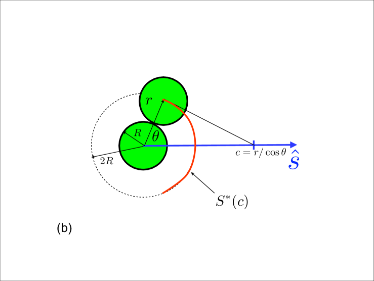
Figure 3: Schematic illustration of the derivation of $P_{\rm B}$ and $P_{\rm C}$. We plot a 2d case for simplicity, although the calculation applies to 3d. (a) $P_{\rm B}$: Background term. The considered particle (green) is located in the center, the closest particle in the $\hat{s}$ direction is at $(r,\theta)$, and the white area is the excluded zone $r<2R$ for the center of any other grain. For a fixed $c$, the grey area with volume $V^{*}(c)$ is the region of the plane $(r^{\prime},\theta^{\prime})$ where $r^{\prime}/\cos\theta^{\prime}<c$. If the particle at $(r,\theta)$ is the Voronoi particle defining the boundary of the Voronoi cell in the $\hat{s}$ direction, then no other particle is in the grey zone in the figure. The computation of $P_{\rm B}$ involves the calculation of the probability that all the remaining particles in the packing are outside the grey excluded volume, $V^{*}(c)$. (b) $P_{\rm C}$: Contact term. The calculation of this term involves the probability to find all the contact particles away from the red area defined by the closest contact particle to the direction $\hat{s}$.

Next, we develop a statistical theory for the probability to find a Voronoi volume in order to calculate the mesoscopic volume function by averaging the single grain function like in Eq. (20). For a given grain, $i$, the calculation reduces to finding the ball $j$ with $\min_{j}r_{j}/\cos\theta_{j}$ where the minimization is over all grains (see Fig. 3 for notation). We consider $r_{j}=r_{ij}$, $\cos\theta_{j}=\hat{s}\cdot\hat{r}_{ij}$, and we set $2R=1$ for simplicity. While the form Eq. (20) is valid for any dimension, the following statistical theory differs for each dimension. In what follows we work in 3d. Results in 2d and large dimension will be presented in future papers.

We consider the minimal particle contributing to the Voronoi volume along the $\hat{s}$ direction at $(r,\theta)$ (see Fig. 3) with

$$c=r/\cos\theta.$$ (21)

We call this particle, the Voronoi particle. Then the quantity to compute is the probability to find all the remaining particles in the packing at a distance larger than $c$ from particle $i$ along the $\hat{s}$ direction. That is, we compute the inverse cumulative distribution function, denoted $P_{>}(c)$, to find all the grains $j$ with $r_{j}/\cos\theta_{j}>c$, and therefore not contributing to the Voronoi volume.

In terms of Fig. 3a, the minimal Voronoi particle located at $c$, determining the Voronoi cell, defines an excluded volume, represented by the gray volume in the figure, where no other particle can be located (otherwise they would contribute to the Voronoi volume). We denote this excluded volume as $V^{*}(c)$. Thus, $P_{>}(c)$ represents the probability that the remaining particles in the packing have $r_{j}/\cos\theta_{j}$ larger than $c$ and therefore are outside the gray volume $V^{*}(c)$ in Fig. 3a.

If we know this inverse cumulative distribution, then the mesoscopic free volume function is obtained as the mean value of $w_{i}^{s}$ over the probability density $-\frac{dP_{>}(c)}{dc}$:

$$w\equiv\langle w_{i}^{s}\rangle_{i}=\langle c^{3}\rangle-1,$$ (22)

and

$$\begin{split}w\equiv\langle w_{i}^{s}\rangle_{i}=\int_{1}^{\infty}(c^{3}-1)\frac{d[1-P_{>}(c)]}{dc}dc=\\ -\int_{1}^{\infty}(c^{3}-1)\frac{dP_{>}(c)}{dc}dc=\\ -\int_{1}^{0}(c^{3}-1)dP_{>}=\int_{0}^{1}(c^{3}-1)dP_{>}.\end{split}$$ (23)

The integration in Eq. (23) ranges from $1$ to $\infty$ with respect to $c$ since the minimum distance for a ball is for $r=1$ and $\theta=0$ giving $c=1$ and the maximum at $r\to\infty$. When changing variables to $dP_{>}$, the limits of integration $c:[1,\infty)$ correspond to the inverse cumulative distribution function $P_{>}:[1,0]$.

Next, we calculate the inverse cumulative distribution $P_{>}(c)$. Considering the Voronoi particle at distance $c$, the remaining balls are in the bulk and in contact with the ball $i$. A crucial step in the calculation is to separate the distribution into two contributions: a contact term, $P_{\rm C}(c)$, and a bulk term, $P_{\rm B}(c)$. This separation is important because it allows one to obtain the dependence of the average volume function on the coordination number. The contact term naturally depends on the number of contacting particles $z$, while the bulk term depends on the average $w$. Since $P_{>}(c)$ represents the probability that all the balls in the packing except the Voronoi ball are outside the grey volume in Fig. 3a, then the geometrical interpretation of the contact and bulk term is the following:

• $P_{\rm B}(c)$ represents the probability that the balls in the bulk are located outside the grey volume $V^{*}(c)$ in Fig. 3a.

• $P_{\rm C}(c)$ represents the probability that the contact balls are located outside the boundary of the grey area marked in red in Fig. 3b and denoted $S^{*}(c)$.

An assumption of the theory is that both contributions are considered independent. Therefore:

$$P_{>}(c)=P_{\rm B}(c)P_{\rm C}(c).$$ (24)

Notice that the meaning of Eq. (24) is the following: we first assume that the Voronoi particle is located at $c$. Then all remaining particles, including contact and bulk particles, are outside the grey excluded zone. This results in the multiplication of the probabilities as in Eq. (24).

4.1 Calculation of $P_{\rm B}(c)$ and $P_{\rm C}(c)$

In order to calculate the distributions $P_{\rm B}$ and $P_{\rm C}$ we apply the following assumptions.

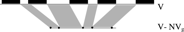
Figure 4: A mapping between hard sphere and ideal gas in the one dimensional system. A system of total volume $V$ of $N$ rods in 1d (hard spheres in 3d with volume $V_{g}$) can be mapped to a system of $N$ points of total size $V-NV_{g}$ by simply removing the size of the balls. This mapping allows to calculate $P_{>}$ exactly in 1d which is shown to be an exponential as in Eq. (26) in the large $N$ limit. For higher dimensions, we cannot just remove the size of the balls $NV_{g}$ since the shape of the balls is important as well. This implies that the exponential probability is an approximation to the real distribution in 3d, as discussed in the text.

We treat the general case of calculating the probability for $N$ particles in a system of volume $V$ to be outside a given volume $V^{*}$ when added at random. In 3d, this probability is nontrivial since the volume occupied by each ball in the packing should be greater than the size of the ball. However, this probability can be calculated exactly in the case of 1d in the large $N$ limit. In 1d, the distribution of possible arrangements of hard-rods corresponds to the distribution of ideal gas particles by removing the volume occupied by the size of the ball as we can see in Fig. 4. Such a mapping is exact in 1d, implying an exponential distribution of the free volume.

The probability to locate one particle at random outside the volume $V^{*}$ in a system of volume $V$ is

$$P_{>}(1)=(1-V^{*}/V).$$

For $N$ independent particles, we obtain:

$$P_{>}(N)=(1-V^{*}/V)^{N}.$$

We set $V^{*}/V=1/x$ and the particle density $\rho=N/V$. Then

$$P_{>}(N)=(1-1/x)^{\rho V}=(1-1/x)^{\rho xV^{*}}.$$ (25)

In the limit of a large number of particles, $x\rightarrow\infty$, we obtain a Boltzmann-like exponential distribution for the probability of $N$ particles to be outside a volume $V^{*}$:

$$P_{>}(N)\propto\exp(-\rho V^{*}),\,\,\,N\to\infty.$$ (26)

While the above derivation is exact in 1d, the extension to higher dimensions is an approximation, since there exist additional geometrical constraints. Even if there is a void with enough volume to be occupied by a particle (the volume of the void is larger or equal than the size of the particle), the constraint imposed by the geometrical shape of the particle (which does not exist in 1d) might prevent the void from being occupied. Nevertheless, in what follows, we assume the exponential distribution of Eq. (26) to be valid in 3d as well.

The background is assumed to be uniform with a mean free bulk particle density given by:

$$\rho(w)=\frac{N}{V-NV_{g}}=\frac{N}{NV_{g}\phi^{-1}-NV_{g}}=\frac{1}{V_{g}w},$$ (27)

where we define the volume fraction $\phi^{-1}=w+1$. Therefore, $P_{\rm B}$ assumes a Boltzmann-like distribution of the form analogous to Eq. (26),

$$P_{\rm B}(c)=\exp\Big{(}-\rho(w)V^{*}(c)\Big{)},$$ (28)

where

$$\begin{split}V^{*}(c)&=2\pi\int\Theta(c-r/\cos\theta)d\vec{r}\\ &=2\pi\int_{1}^{\infty}\int_{0}^{\pi/2}\Theta(c-r/\cos\theta)r^{2}\sin\theta d\theta dr\\ &=2\pi\int_{1}^{c}r^{2}\int_{0}^{\arccos(r/c)}\sin\theta d\theta dr\\ &=2\pi\int_{1}^{c}(1-r/c)r^{2}dr\end{split}$$ (29)

is the volume of the grey area in Fig. 3a. We obtain:

$$V^{*}(c)=V_{g}\left((c^{3}-1)-3(1-\frac{1}{c})\right).$$ (30)

Therefore,

$$P_{\rm B}(c)=\exp\Big{[}-\frac{(c^{3}-1)-3(1-1/c)}{w}\Big{]}.$$ (31)

The derivation of the surface term, $P_{\rm C}(c)$, is analogous to that of the volume term. $P_{C}(c)$ is assumed to have the same exponential form, analogous to the background form of $P_{B}(c)$, Eq. (28), despite not having the large number approximation leading to Eq. (26):

$$P_{\rm C}(c)=\exp\Big{(}-\rho_{S}(z)S^{*}(c)\Big{)},$$ (32)

where

$$S^{*}(c)=2\pi\int_{0}^{\arccos(1/c)}\sin\theta d\theta=2\pi(1-\frac{1}{c}),$$ (33)

is the excluded area marked in red in Fig. 3b.

To define $\rho_{S}(z)$ we first follow the analogy with the bulk density Eq. (27), $\rho(w)$ to obtain the mean free surface particle density on the sphere with $z$ contacting particles:

$$\rho_{S}(z)=\frac{z}{4\pi-zS_{\rm occ}},$$ (34)

where $S_{\rm occ}=2\pi\int_{0}^{\pi/6}\sin\theta d\theta=2\pi a$ is the surface occupied by a single contact ball, with $a=1-\sqrt{3}/2$ a small value.

However, we notice that the analogy with Eq. (26) is more difficult to justify here since the large number limit is lacking for the surface term: the maximum number of contacting spheres, the so-called kissing number, is 12 and for disordered packings is 6 in average. Thus, rather than considering Eq. (32) as the exact form of the surface term, we take the exponential form as a simple variational Ansatz, where the surface density $\rho_{S}(z)$ is the variational parameter which has to be corrected from Eq. (34) due to the small number of the balls on the surface.

A more physical definition of $\rho_{S}(z)$ is a mean free density representing the inverse of the average of $S^{*}(c)$: $\langle S^{*}(c)\rangle$. The meaning of $\langle S^{*}(c)\rangle$ for a given number of contacting particles is the following: add $z$ contact particles at random around a central sphere. The average of the solid angles of the gaps left between nearest neighbor contacting spheres is $\langle S^{*}(c)\rangle$ (see Fig. 5). Indeed we obtain:

$$\begin{split}\langle S^{*}\rangle&=\int_{1}^{\infty}S^{*}(c)\frac{d[1-P_{C}(c)]}{dc}dc\\ &=\int_{1}^{\infty}S^{*}(c)\rho_{S}\exp(-\rho_{S}S^{*}(c))\frac{dS^{*}}{dc}dc\\ &=\rho_{S}\int_{0}^{2\pi}S^{*}\exp(-\rho_{S}S^{*})dS^{*}\\ &\approx\rho_{S}\int_{0}^{\infty}S^{*}\exp(-\rho_{S}S^{*})dS^{*}\\ &=1/\rho_{S}\end{split}$$ (35)

Then, the surface density is replaced by the following definition:

$$\rho_{S}=\frac{1}{\left<S^{*}\right>}$$ (36)

Under these considerations, in order to estimate the value of $\rho_{S}(z)$ we first consider a single particle approximation. We calculate the mean of $S^{*}$ for a single particle $z=1$, which gives $\left<S^{*}\right>=2\pi$, since $S^{*}$ ranges uniformly from $0$ to $4\pi$. We note that the value is different from the prediction of Eq. (34) in the large number limit. Since we expect $\rho_{S}(z)$ to be proportional to $z$, under a single particle approximation we find:

$$\rho_{S}(z)\approx\frac{z}{2\pi},\,\,\,\,\,\,\mbox{single particle approximation}.$$ (37)

Simulations considering many $z$ contacting particles suggest that corrections from the single particle approximation are important for larger $z$. Indeed, a more precise value is obtained from simulations:

$$\rho_{S}(z)\approx\frac{z}{2\pi}\frac{\sqrt{3}}{2},\,\,\,z>1,$$ (38)

deviating from the single particle approximation of Eq. (37). This numerical calculation consists of adding $z$ random, non-overlapping, equal-size spheres at the surface of a ball. For every fix $z$, the sphere closest to the direction $\hat{s}$ defines the free angle $\theta^{*}$ and the surface $S^{*}=2\theta^{*}$ (see Fig. 5). Thus, the idea is to measure the mean gap, $\left<S^{*}\right>$, left by $z$ contacting particles along the $\hat{s}$ direction. As seen in Fig. 6, simulations show that the more precise value, Eq. (38) is valid rather than the single particle approximation, Eq. (37).

This many-particle result can be explained by adding a small correction term from the area occupied by one particle into Eq. (37). In the case of many contact particles, $z>1$, many body constraints imply that the surface, $\left<S^{*}\right>$, should be corrected by the solid angle extended by a single ball, and at the same time reduced by the increasing number of contacting particles. Thus, up to first order approximation,

$$\left<S^{*}\right>\approx(2\pi+S_{\rm occ})/z.$$

This analysis provides a correction to the surface term which can be approximated as

$$\begin{split}\rho_{S}(z)=&\frac{z}{2\pi+S_{\rm occ}}=\frac{z}{2\pi(1+a)}\\ \approx&\frac{z}{2\pi}(1-a)=\frac{z}{2\pi}\frac{\sqrt{3}}{2},\,\,\,z>1,\end{split}$$ (39)

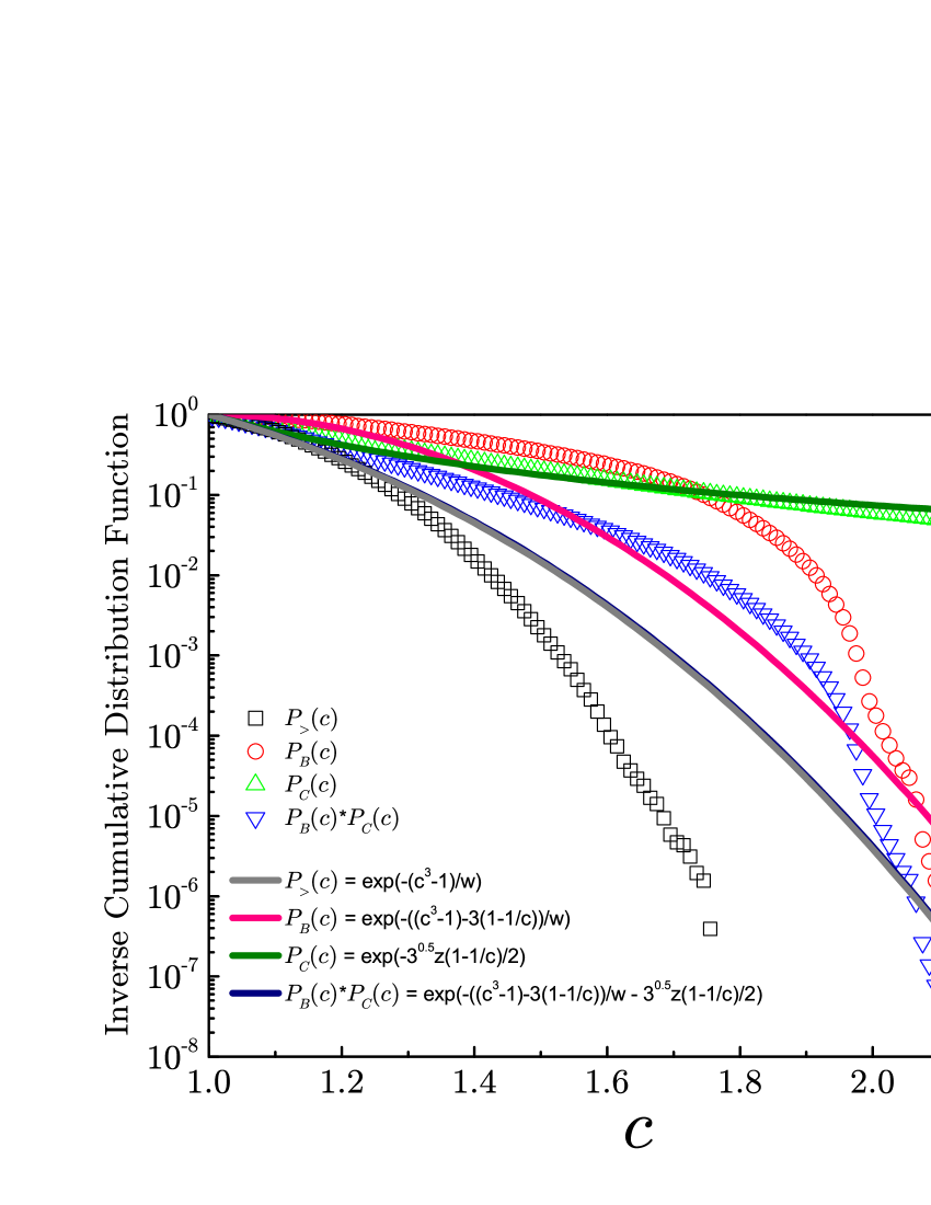
Figure 8: Comparison between theory and simulations for the inverse cumulative distributions, $P_{\rm B}(c),P_{\rm C}(c)$, $P_{\rm B}(c)\times P_{\rm C}(c)$ and $P_{>}(c)$ for a packing at the frictionless point with $z=6$ as explained in Jamming II [6]. The choice of a frictionless packing to test the distribution of volumes is due to the fact that these packings are independent of the compactivity as will be shown in Jamming II. In general such an equation for the distribution of $c$ should be tested by generating local packings by randomly adding $z$ balls surrounding a given sphere.

It is clear that the above derivation is by no means exact. It merely interprets the origin of the correction from the single particle approximation in order to obtain a proper estimation of the surface density. The obtained value agrees very well with the computer simulations results of Fig. 6 and Eq. (38), and therefore we use it to define $P_{\rm C}(c)$. In comparison with numerical simulations, the derived form of $P_{\rm C}(c)$ compares well as we will show in Fig. 8. Furthermore, the predicted average volume fraction compares well with experiments on random close packings.

From Eqs. (32), (33) and (39), we obtain the surface term:

$$P_{\mathrm{C}}(c)=\exp\Big{[}-\sqrt{3}z(1-1/c)/2\Big{]},$$ (40)

and the inverse cumulative distribution of volumes takes the form:

$$P_{>}(c)>=\exp\left[-\frac{1}{w}\left((c^{3}-1)-3(1-\frac{1}{c})\right)-\frac{\sqrt{3}}{2}z(1-\frac{1}{c})\right].$$ (41)

5 The mesoscopic volume function

Substituting Eq. (41) into Eq. (23), we obtain a self-consistent equation to calculate the average free volume, $w$:

$$\begin{split}w=\int_{0}^{1}(c^{3}-1)\,\,\,d\exp\Big{[}-\frac{1}{w}\Big{(}(c^{3}-1)-3(1-\frac{1}{c})\Big{)}-\\ \frac{\sqrt{3}}{2}z(1-\frac{1}{c})\Big{]}.\end{split}$$ (42)

Since

$$w=\int_{0}^{1}(c^{3}-1)d\exp[-(c^{3}-1)/w],$$ (43)

then Eq. (42) can be solved exactly, leading to an analytical form of the free average volume function, under the approximations of the theory. The fact that we can solve this equation exactly is a fortuitous event. It is worth mentioning that an analogous analysis performed in 2d as well as in infinite dimensions does not lead to an analytical solution of the self-consistent equation (42) and therefore only numerical solutions are possible for the average volume function in those dimensions under similar assumptions as used in 3d.

To solve Eq. (42) we start from the identity:

$$\int_{0}^{\infty}\frac{x}{w}\exp(-\frac{x}{w})dx=1.$$ (44)

Then we find:

$$\begin{split}1=\int_{0}^{1}\frac{1}{w}\Big{(}(c^{3}-1)-\alpha(1-\frac{1}{c})\Big{)}\times\\ d\exp\left[-\frac{1}{w}\left((c^{3}-1)-\alpha(1-\frac{1}{c})\right)\right],\end{split}$$ (45)

where $\alpha=3-wz\sqrt{3}/2$. Or

$$\begin{split}0&=\int_{0}^{1}\frac{1}{w}(c^{3}-1)d\exp\left[-\frac{1}{w}\left((c^{3}-1)-\alpha(1-\frac{1}{c})\right)\right]-1\\ &=\alpha\int_{0}^{1}\frac{1}{w}\left(1-\frac{1}{c}\right)d\exp\left[-\frac{1}{w}\left((c^{3}-1)-\alpha(1-\frac{1}{c})\right)\right].\end{split}$$ (46)

The second integration in the right hand side is equal to zero only at $w=0$ or $w\rightarrow\infty$, corresponding to two trivial solutions at $\phi=1$ and $\phi=0$, respectively. The only non-trivial solution happens at $\alpha=0$, and therefore we find

$$w(z)=\frac{2\sqrt{3}}{z}\,\,\,\,\Rightarrow\,\,\,\,W(z)=\frac{2\sqrt{3}}{z}V_{g}.$$ (47)

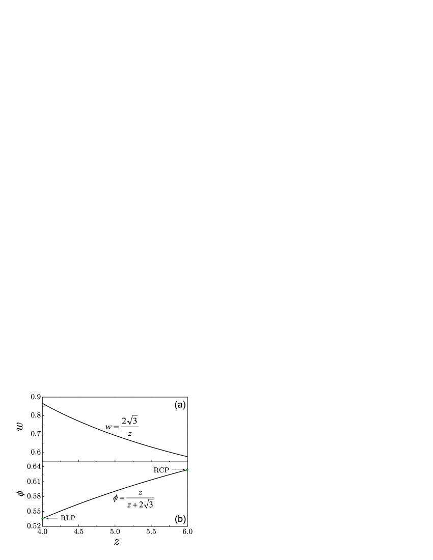
Figure 7: (a) Mesoscopic volume function of granular matter, $w(z)$ versus $z$. (b) Equation of state relating the volume fraction and coordination number in the limit of infinite compactivity.

We arrive at a mesoscopic volume function (plotted in Fig. 7a) which is more amenable to a statistical mechanics approach for jammed matter. Equation (47) is a coarse-grained “Hamiltonian” or volume function that replaces the microscopic Eq. (14) to describe the mesoscopic states of jammed matter. While Eq. (14) is difficult to treat analytically in statistical mechanics, the advantage of the mesoscopic Eq. (47) is that it can easily be incorporated into a partition function since it depends only on $z$ instead of all degrees of freedom ${\vec{r}}_{i}$.

If the system is fully random, so that we can extend the assumption of uniformity from the mesoscopic scales to the macroscopic scales, we arrive to an equation of state relating $\phi^{-1}=w+1$ with $z$ as:

$$\phi=\frac{z}{z+2\sqrt{3}}.$$ (48)

Thus, Eq. (48), plotted in Fig. 7b, can be interpreted as a equation of state for fully random jammed matter. We recall that it has been obtained under the approximation of a packing achieving a completely random state; the proper test of such an equation would be to add spheres at random and observe their distribution and average values. In a second paper of this series [6] we will show that it corresponds to the equation of state in the limit of infinite compactivity when the system is fully randomized. Indeed, Eq. (48) already provides the density of random loose packings and random close packings when the coordination number is replaced by the isostatic limits of 4 and 6, for infinitely rough and frictionless particles, respectively.

So far, our analysis only includes geometrical constraints, but has not made use of the mechanical constraint of jamming. The jamming condition can be introduced through the condition of isostaticity which applies to the mechanical coordination number, $Z$, for rigid spherical grains [7]. For isostatic packings the mechanical coordination number is bounded by $Z=d+1=4$ and $Z=2d=6$ and we obtain the minimum and maximum volume fraction from Eq. (48) as $\phi_{\rm RLP}=4/(4+2\sqrt{3})\approx 0.536$ and $\phi_{\rm RCP}=6/(6+2\sqrt{3})\approx 0.634$ as shown in Fig. 7b. We identify these limits as the random close packing (RCP) and random loose packing (RLP) fractions (the maximum and minimum possible volumes of random packings of spherical particles). This result is fully explored in Jamming II [6] where the phase space of jammed configurations is obtained using Edwards statistical mechanics of jammed matter based on Eq. (47). We note that the mechanical coordination, $Z$, is not the same as the geometrical one, $z$ (see [6] for details), and an equation of state of jammed matter should be a relation between state variables, such as average global volume fraction $\phi$ and mechanical coordination number $Z$. However, it can be shown that in the limit of infinite compactivity, the mechanical coordination number $Z$ is identical to the geometrical coordination number $z$, and the equation of state in this case has the same form of Eq. (48). Thus for now, it suffices to say that we can obtain the two packing limits from Eq. (48) in the case of fully random systems of infinite compactivity.

The experimental studies of [5] on the free volume versus coordination number of grains in tomography studies of random packings of spheres support Eq. (48) (see Fig. 6 in [5]).

5.1 Quasiparticles

Equation (47) should be interpreted as representing quasiparticles with free volume $w$ and coordination number $z$. When a grain jams in a packing, it interacts with other grains. The role of this interaction is assumed in the calculation of the volume function (47) and is implicit in the coarse-graining procedure explained above. Thus, the quasiparticles can be considered as particles in a self-consistent field of surrounding jammed matter. In the presence of this field, the volume of the quasiparticles depends on the surrounding particles, as expressed in Eq. (47). The assembly of quasiparticles can be regarded as a set of non-interacting particles (when the number of elementary excitations is sufficiently low). The jammed system can be considered as an ideal gas of quasiparticles and a single particle partition function can be used to evaluate the ensemble. These ideas are exploited in the definition of the partition function leading to the solution of the phase diagram discussed in Jamming II [6].

6 Numerical Tests

In this section, we wish to test some predictions and approximations of the theory and propose the necessary improvements where needed. The purpose of this calculation is, first, to evaluate the predictions of the theory regarding the inverse cumulative volume distributions, and, second, to test whether the background distribution is independent of the contact distribution by comparing $P_{\rm B}(c)\times P_{\rm C}(c)$ with $P_{>}(c)$.

It is important to note that the predictions of the mesoscopic theory refer to quasiparticles as discussed above. The quasiparticles of free volume Eq. (47) of fix coordination number can be considered as the building blocks or elementary units of jammed matter. To properly study their properties and test the predictions and approximations of the present theory one should in principle isolate the behavior of the quasiparticles and study their statistical properties such as the distribution of volumes and their mean value as a function of coordination number. Such a study is being carried out and may lead to a more precise solutions than the one presented in the present paper.

Nevertheless, in what follows we take an approximate numerical route and study the behavior of quasiparticles directly from computer generated packings with Molecular Dynamics. While such packings already contain the ensemble average of the quasiparticle, we argue that in some limits they could provide statistics for isolated quasiparticles, at least approximately. This is due to a result that needs to wait until Jamming II [6], where we find that for a system of frictionless packings there is a unique state of jamming at the mesoscopic level and therefore the compactivity and the ensemble average does not play a role, at least under the mesoscopic approximation developed here. Therefore, below, we use frictionless packings in order to test the theory. We note, though, that the conclusions of this section remain approximative, waiting for a more precise study of the packings of fixed coordination number.

We prepare a frictionless packing at the jamming transition with methods explained in Jamming II. The packing consists of 10,000 spherical particles interacting with Hertz forces. In the simulation, we pick up a direction $\hat{s}$ randomly, and collect $c_{b}$ and $c_{c}$ from the balls, as follows:

$$c_{b} = \min_{\hat{s}\cdot\hat{r}_{ij}>0}\frac{r_{ij}}{2\hat{s}\cdot\hat{r}_{ij}},r_{ij}>2R,$$ (49)

$$c_{c} = \min_{\hat{s}\cdot\hat{r}_{ij}>0}\frac{r_{ij}}{2\hat{s}\cdot\hat{r}_{ij}},r_{ij}\leq 2R.$$

Thus, for a given direction, we find two minimum values of $c$ independently as $c_{b}$ and $c_{c}$ over all particles in the packing. We then collect data for 400 different directions. The $c_{b}$ is only provided by the balls in the background, and $c_{c}$ is only provided by the balls in contact. From the probability density, we then calculate the cumulative probability to find a ball at position $r$ and $\theta$ such that $r/\cos\theta>c$. That is, we calculate the cumulative distribution of $c_{b}$ and $c_{c}$ individually, i.e., $P_{\rm B}(c_{b})$ and $P_{\rm C}(c_{c})$.

The inverse cumulative distributions are plotted Fig. 8 showing that the theory approximately captures the trend of these functions but deviations exist as well, especially for $c$ values larger than its average. The contact term $P_{\rm C}(c)$ is well approximated by the theory supporting the approximations involved in the calculation of the surface density term, Eq. (39). The background term shows deviations for larger $c$; for smaller $c$ the theory is not too far from simulations. From Fig. 8 we notice that $P_{>}(c)$ is well reproduced by the theory up to a value of 10% of its peak value.

It is important to note that the mesoscopic volume function, $w$, is extracted from the mean value of $\langle w^{s}\rangle$ as $w=\langle w^{s}\rangle=\langle c^{3}\rangle-1$. While some deviations are found in the inverse cumulative distribution, we find that the average value of the volumes are well approximated by the theory. Indeed, we find that the deviations from the theoretical probabilities for $w^{s}>\langle w^{s}\rangle$ appear not to contribute significantly towards the average volume function.

For instance, the packing in Fig. 8 has a volume fraction $\phi=0.64$ as measured from the particle positions. This value agrees with the average $\langle w^{s}\rangle$ obtained from the prediction of the probability distribution $P_{>}(c)$. We find $\langle c^{3}\rangle$ = 1.561, then $\langle w^{s}\rangle$ = $\langle c^{3}\rangle-1=0.561$ and $\phi=1/\langle c^{3}\rangle=1/(\langle w^{s}\rangle+1)=0.641$ in agreement with the volume fraction of the entire packing obtained from the position of all the balls, $0.64$.

Thus, the present theory gives a good approximation to the average Voronoi volume needed for the mesoscopic volume function, even though the full distribution presents deviations from the theory. In order to capture all the moments of the distribution a more refined theory is needed. Such a theory will include the corrections to the exponential forms of $P_{\rm B}(c)$ and $P_{\rm C}(c)$ and their correlations. The main result of the mesoscopic theory, being the average Voronoi volume decreasing with the number of contacts, is not affected by the assumptions of the theory for the full probability distribution.

The correlations between the contact and bulk term are quantified by comparing $P_{\rm B}(c)\times P_{\rm C}(c)$ with $P_{>}(c)$ in Fig. 8. From the figure we see that below and around the mean $\langle c\rangle$, the full distribution is close to the theoretical result while deviations appear for larger $c$. Further testing of the existence of correlations between $P_{\rm B}(c)$ and $P_{\rm C}(c)$ is obtained by calculating the product-moment coefficient of Pearson’s correlation as follows.

The Pearson’s coefficient is:

$$r^{2}=\frac{{S_{bc}}^{2}}{S_{bb}S_{cc}},$$ (50)

where $S_{bb}=\Sigma({c_{b}}^{2}-{{\bar{c}}_{b}}^{2})$, $S_{cc}=\Sigma({c_{c}}^{2}-{\bar{c}_{c}}^{2})$, and $S_{cb}=\Sigma(c_{b}c_{c}-\bar{c}_{b}\bar{c}_{c})$. We find that the Pearson coefficient $r^{2}=0.0173$ is close to zero, meaning that the correlations between $P_{B}(c)$ and $P_{C}(c)$ are weak.

The present numerical results imply that the current assumptions of the theory are reasonable. The conclusions are that while the cumulative distributions present deviations from the theory in their tails, the average value of the Voronoi volumes are well captured by the approximations of the theory, therefore providing an accurate value for the volume function.

More importantly, the present approach indicates a way to improve the theory to provide more accurate results. Our current studies indicate that an exact solution of the distribution, $P_{>}(c)$, may be possible up to the second coordination shell of particles, for a fixed z-ensemble. Due to the fact that the range of Voronoi cell is finite, it is possible to work out a description for the finite, but large, number of degrees of freedom for both disordered and ordered packings through computational linear programming, in principle. This approach is related to the Hales’ proof of the Kepler conjecture [8]. The present theory is a mean-field version in terms of the restricted description of the disordered packings, which allows us to reduce the dimensionality of the original problem in order to write down the analytic form of the volume function in reasonable agreement with known values of RCP and RLP. The present approximations of the theory are further supported by agreement between the obtained form of the volume function and the empirical findings of the experiments of [5]. In a future paper we will present a more exact theory of the volume fluctuations capturing not only the mean value but also higher moments.

It is of interest to test the formula Eq. (47) with the well-known example of the FCC lattice at $z=12$ to assess the approximations of the theory. At this limiting number of neighbors the entire class of attainable orientational Voronoi cells have volumes in a very narrow range around $0.7V_{g}$ which is larger than the prediction from Eq. (47). The free volume of the FCC Voronoi cell is $0.35135$ while the mesoscopic volume function for $z=12$ gives $2\sqrt{3}/12=0.2886$, below the real value. We explain this discrepancy since the current theory is developed under the assumption of isotropic packings. Isotropic packings are explicitly taken into account in the theory considering the orientational Voronoi volume ${\cal W}_{i}^{s}$ (along a direction $\hat{s}$) as a simplification of the full Voronoi volume, ${\cal W}_{i}^{\rm vor}$. Such a simplification is meaningful for isotropic packings but fails for anisotropic or ordered packings. Indeed, in the case of packings with strong angular correlations, the “weak-coupling” hypothesis employed here does not work well. The extension of the current theory to anisotropic packings, such as the FCC lattice at $z=12$, can be carried out, but remains outside of the scope of the present work. In this case, the full Voronoi volume of Eq. (14) must be used.

Eventually a volume function that accounts for disordered and ordered packings is very important. This volume function could test the existence of phase transition between the ordered and disordered phases. The theory we propose here is a quasiparticle version in terms of the restricted description of the disordered packings, which allows us to reduce the dimensionality of the original problem in order to write down the analytic form of the volume function. The fact that Eq. (47) does not predict correctly the volume of FCC but does predict correctly the volume of RCP raises the interesting possibility that there could be a phase transition at RCP, an intriguing possibility which is being explored at the moment.

7 Summary

In summary, we present a plausible volume function describing the states of jammed matter. The definition of ${\cal W}_{i}$ is purely geometrical and, therefore, can be extended to unjammed systems such as colloids at lower concentrations. In its microscopic definition, the volume function is shown to be the Voronoi volume per particle, and an analytical formula is derived for it. However this form is still intractable in a statistical mechanics analysis. We then develop a mesoscopic version of ${\cal W}_{i}$ involving coarse graining over a few particles that reduces the degrees of freedom to a single variable, $z$. This renders the problem within the reach of analytical calculations. The significance of our results is that they allow the development of a statistical mechanics to predict the observables by using the volume function in a Boltzmann-like probability distribution of states [1] when the analysis is supplemented by the jamming condition ’a la Alexander’ [7]; which we propose in [6] to be the isostatic condition for rigid particles.

Acknowledgements. This work is supported by NSF-CMMT, and DOE Geosciences Division. We thank J. Brujić for inspirations and C. Briscoe for a critical reading of this manuscript.

Figure 5: The calculation of the surface term $P_{\rm C}$ involves the mean free surface density for a given $z$ (=4 in this example) obtained from the angle $\theta^{*}$. Note that we show the 2d case for simplicity, but the $\theta^{*}$ corresponds to a solid angle in 3d.

Figure 6: A numerical calculation using packing of spheres confirms that $2\pi\rho_{S}(z)=2\pi/\langle S^{*}\rangle$ (dots) slightly deviates from the single particle estimation as $z$ (dash line), and is much better approximated by $(\sqrt{3}/2)z$ with particle size correction (solid line).

References

- [1] S. F. Edwards, in Granular matter: an interdisciplinary approach (ed A. Mehta) 121-140 (Springer-Verlag, New York, 1994).
- [2] R. C. Ball and R. Blumenfeld, Phys. Rev. Lett. 88, 115505 (2002).
- [3] R. Blumenfeld, Eur. Phys. J. B 29, 261 (2005).
- [4] S. F. Edwards and D. Grinev, Chem. Eng. Sci. 56, 5451 (2001).
- [5] T. Aste, M. Saadatfar and T. J. Senden, J. Stat. Mech., P07010 (2006).
- [6] C. Song, P. Wang and H. A. Makse, Nature 453, 606 (2008).
- [7] S. Alexander, Phys. Rep. 296, 65 (1998).
- [8] T. C. Hales, The Kepler conjecture. http://arxiv.org/abs/math.MG/9811078