Superintegrability of the Caged Anisotropic Oscillator

Abstract

We study the Caged Anisotropic Harmonic Oscillator, which is a new example of a superintegrable, or accidentally degenerate Hamiltonian. The potential is that of the harmonic oscillator with rational frequency ratio ($l:m:n$), but additionally with barrier terms describing repulsive forces from the principal planes. This confines the classical motion to a sector bounded by the principal planes, or cage. In 3 degrees, there are five isolating integrals of motion, ensuring that all bound trajectories are closed and strictly periodic. Three of the integrals are quadratic in the momenta, the remaining two are polynomials of order $2(l+m-1)$ and $2(l+n-1)$ . In the quantum problem, the eigenstates are multiply degenerate, exhibiting $l^{2}m^{2}n^{2}$ copies of the fundamental pattern of the symmetry group $SU(3)$.

I Introduction

The subject of accidental degeneracy has fascinated physicists since the early days of the quantum theory. It has long been known that the trajectory in an $r$-squared force (the Coulomb or Kepler problem) is a conic section, so that every bound orbit is an ellipse and therefore closed and strictly periodic. The advent of the quantum theory saw the deduction of the eigenfunctions for the Hydrogen atom and thence the realization that the bound states of the Coulomb problem are degenerate  Pa26 (1, 2, 3). This accidental degeneracy is a consequence of a hidden symmetry group SO(4) that is not manifest to the eye. It causes all bound trajectories to be closed in the classical problem.

There is a fundamental connection between accidental degeneracy and the separability of the Schrödinger or the Hamilton-Jacobi equations in more than one coordinate system and therefore the existence of additional conserved quantities or integrals of motion. This is mentioned in a number of the famous texts of the old quantum theory – such as Born’s Mechanics of the Atom and Sommerfeld’s Atomic Structure and Spectral Lines. For example, the Coulomb problem is separable in both spherical polar and rotational parabolic coordinates. The former leads to the conservation of the angular momentum vector, the latter to the conservation of the Laplace-Runge-Lenz vector. The quantum mechanical operators close to form the algebra of SO(4) (see, for example, Ar76 (4) for a review). The accidental degeneracy is a consequence of additional integrals of motion We93 (5) and so such systems are often called superintegrable Te05 (6).

Systematic investigations of all the possible combinations of coordinate systems for which the Schrödinger and Hamilton-Jacobi equation can separate have now been carried out Fr65 (7, 8, 9). In three degrees of freedom, this yields 13 distinct superintegrable systems, all of which have classical integrals of motion or quantum operators that are quadratic in the canonical momenta and all of which exhibit accidental degeneracy. This includes familiar systems such as the Coulomb problem and the isotropic harmonic oscillator.

Nonetheless, this does not provide a comprehensive explanation of the phenomenon of superintegrability. For example, in three degrees of freedom, the Hamiltonian of the anisotropic harmonic oscillator with rational frequency ratio is

$$H=\frac{1}{2}(p_{x}^{2}+p_{y}^{2}+p_{z}^{2})+k(l^{2}x^{2}+m^{2}y^{2}+n^{2}z^{2}),$$ (1)

where $l,m$ and $n$ are integers and $k$ is a constant. The Hamilton-Jacobi or Schrödinger equations clearly separate in rectangular Cartesians. If $l:m:n=2:1:1$, then the Hamiltonian also separates in the rotational parabolic and elliptic cylindrical coordinate systems Ev90 (9), giving rise to additional conserved quantities and accidental degeneracy. However, if $l+m+n>4$, then the Hamiltonian is still superintegrable Ja40 (10, 11, 12), even though it now only separates in rectangular Cartesians. Further examples of systems which are superintegrable but not separable in more than one coordinate system include the Calogero-Moser problem Ad77 (13, 14) and the generalized Coulomb problem VE08 (15).

The purpose of this paper is to introduce another superintegrable Hamiltonian, closely related to (1), namely

$$H=\frac{1}{2}(p_{x}^{2}+p_{y}^{2}+p_{z}^{2})+k(l^{2}x^{2}+m^{2}y^{2}+n^{2}z^{2})+\frac{k_{1}}{x^{2}}+\frac{k_{2}}{y^{2}}+\frac{k_{3}}{z^{2}}$$ (2)

We shall refer to this as “the Caged Anisotropic Oscillator”, as the presence of the barrier terms confines the motion to an octant defined by the principal planes. When $l=m=n=1$, this becomes the Smorodinsky-Winternitz system, on which there is an extensive literature  Fr65 (7, 16, 17).

Like the Smorodinsky-Winternitz system, the Caged Anisotropic Oscillator has five integrals of motion and it exhibits accidental degeneracy in quantum mechanics. However, unlike the Smorodinsky-Winternitz system, the Hamilton-Jacobi and Schrödinger equations only separate in rectangular Cartesians. In this paper, we demonstrate that the Hamiltonian (2) is superintegrable using the method of projection in §2. Then we discuss both the classical and quantum problems in some detail in §3 and §4 respectively.

II Proof of Superintegrability

Let us start with the observation that the commensurate anisotropic oscillator in $N$ dimensions possesses $2N-1$ functionally independent integrals of motion, equal to the $N$ energies of each individual oscillator and the $N-1$ phases differences between them AW02 (11). In six dimensions, we have

$$H_{6}=\sum_{i=0}^{6}\left(\frac{1}{2}p_{i}^{2}+kn_{i}^{2}s_{i}^{2}\right)$$ (3)

where the $n_{i}$ are positive integers and the $s_{i}$ are Cartesian coordinates. If we now introduce coordinates $(x,y,z,\theta_{x},\theta_{y},\theta_{z})$ according to

$$s_{1} = x\cos\theta_{x},\qquad s_{2}=x\sin\theta_{x}$$

$$s_{3} = y\cos\theta_{y},\qquad s_{4}=y\sin\theta_{y}$$

$$s_{5} = z\cos\theta_{z},\qquad s_{6}=z\sin\theta_{z}$$

and let the frequencies $n_{1}=n_{2}=l$, $n_{3}=n_{4}=m$, $n_{5}=n_{6}=n$, we have the Hamiltonian

$$H=\frac{1}{2}\left(p_{x}^{2}+p_{y}^{2}+p_{z}^{2}+\frac{p_{\theta_{x}}^{2}}{x^{2}}+\frac{p_{\theta_{y}}^{2}}{y^{2}}+\frac{p_{\theta_{z}}^{2}}{z^{2}}\right)+k(l^{2}x^{2}+m^{2}y^{2}+n^{2}z^{2})$$ (4)

Since the coordinates $(\theta_{x},\theta_{y},\theta_{z})$ are ignorable we can set the conjugate momenta to constants. Making the substitutions $p_{\theta_{x}}^{2}=k_{1}$, $p_{\theta_{y}}^{2}=k_{2}$, $p_{\theta_{z}}^{2}=k_{3}$ gives us the Caged Harmonic Oscillator Hamiltonian (2).

For the Hamiltonian in 6 dimensions given by (3), every bound trajectory is closed. Similarly, in the reduced 3 degrees of freedom Hamiltonian (2), every bound trajectory is also closed and the system is still superintegrable.

Figure 1: A typical orbit for a frequency ratio of $l:m:n=1:1:3$.

Figure 2: A typical orbit for a frequency ratio of $l:m:n=1:2:3$.

III Classical Mechanics

III.1 The Integrals of Motion

The Hamiltonian (2) clearly separates in rectangular Cartesian coordinates to give the first three integrals of motion as the three energies of oscillation

$$I_{1} = \frac{1}{2}p_{x}^{2}+kl^{2}x^{2}+\frac{k_{1}}{x^{2}}$$ (5)

$$I_{2} = \frac{1}{2}p_{y}^{2}+km^{2}y^{2}+\frac{k_{2}}{y^{2}}$$ (6)

$$I_{3} = \frac{1}{2}p_{z}^{2}+kn^{2}z^{2}+\frac{k_{3}}{z^{2}}$$ (7)

As the system is separable in these coordinates, it is easy to see that the trajectories of the orbits are (c.f. Ev90 (9))

$$x^{2} = \frac{I_{1}}{2l^{2}k}+\left(\frac{I_{1}^{2}}{4l^{4}k^{2}}-\frac{k_{1}}{l^{2}k}\right)^{1/2}\cos(\sqrt{8k}l(t-t_{0}))$$ (8)

$$y^{2} = \frac{I_{2}}{2m^{2}k}+\left(\frac{I_{2}^{2}}{4m^{4}k^{2}}-\frac{k_{2}}{m^{2}k}\right)^{1/2}\cos(\sqrt{8k}m(t-t_{0})+c_{1})$$ (9)

$$z^{2} = \frac{I_{3}}{2n^{2}k}+\left(\frac{I_{3}^{2}}{4n^{4}k^{2}}-\frac{k_{3}}{n^{2}k}\right)^{1/2}\cos(\sqrt{8k}n(t-t_{0})+c_{2})$$ (10)

where $t_{0}$ and the $c_{i}$ are constants. The remaining two integrals are the phase differences between the orbits, say $c_{1}$ and $c_{2}$. If we say too that $|m-l|<|n-l|<|n-m|$, then the integrals are also of lowest order possible in the momenta. First, let us define

$$\xi\doteq\frac{x^{2}-\alpha}{A} = \cos(\sqrt{8k}l(t-t_{0}))$$ (11)

$$\eta\doteq\frac{y^{2}-\beta}{B} = \cos(\sqrt{8k}m(t-t_{0})+c_{1})$$ (12)

$$\zeta\doteq\frac{z^{2}-\gamma}{C} = \cos(\sqrt{8k}n(t-t_{0})+c_{2})$$ (13)

where $\alpha=I_{1}/(2l^{2}k)$, $\beta=I_{2}/(2m^{2}k)$ and $\gamma=I_{3}/(2n^{2}k)$ and

$$A = \left(\frac{I_{1}^{2}}{4l^{4}k^{2}}-\frac{k_{1}}{l^{2}k}\right)^{1/2},\qquad\qquad B=\left(\frac{I_{2}^{2}}{4m^{4}k^{2}}-\frac{k_{3}}{m^{2}k}\right)^{1/2},$$

$$C = \left(\frac{I_{3}^{2}}{4n^{4}k^{2}}-\frac{k_{3}}{n^{2}k}\right)^{1/2}$$ (14)

The derivation of both integrals is similar and will be demonstrated with the case of $c_{1}$. The first phase difference is given by (c.f., the discussion of the anisotropic oscillator in BP96 (12))

$$c_{1}=\arccos\eta-\frac{m}{l}\arccos\xi$$ (15)

Taking the cosine gives

$$\cos(lc_{1}) = \cos(l\arccos\eta)\cos(m\arccos\xi)+\sin(l\arccos\eta)\sin(m\arccos\xi)$$ (16)

$$= T_{l}(\eta)T_{m}(\xi)+\frac{\dot{\xi}\dot{\eta}}{8km^{2}l^{2}}T^{\prime}_{l}(\eta)T^{\prime}_{m}(\xi)$$

where $T_{l}$ and $T_{m}$ are the Chebyshev polynomials of the first kind  Er (18) and $T^{\prime}_{l}$ and $T^{\prime}_{m}$ are their derivatives with respect to the arguments $\eta$ and $\xi$. The time derivatives $\dot{\xi}$ and $\dot{\eta}$ are equal to $2xp_{x}/A$ and $2yp_{y}/B$ respectively. It is more convenient to express the integral as

$$I_{4}=(2k)^{l+m}A^{m}B^{l}\cos(lc_{1})$$ (17)

which is of order $2(l+m)$ in the momenta, but can be reduced to order $2(l+m-1)$ since the two highest powers of the momenta can be removed though a combination of the energy integrals.

The corresponding integral for the second phase difference $c_{2}$ is

$$I_{5}=(2k)^{l+n}A^{n}C^{l}\cos(lc_{2})$$ (18)

where

$$\cos(lc_{2})=T_{l}(\zeta)T_{n}(\xi)+\frac{\dot{\xi}\dot{\zeta}}{8kn^{2}l^{2}}T^{\prime}_{l}(\zeta)T^{\prime}_{n}(\xi)$$ (19)

which can be reduced to order $2(l+n-1)$ in the momenta. It is easy to verify that both $I_{4}$ and $I_{5}$ are integrals of motion by showing that the Poisson bracket with the Hamiltonian vanishes. They are also functionally independent, as may be verified by computing the rank of the appropriate Jacobian.

Figure 3: A typical orbit for a frequency ratio of $2:3:4$.

Figure 4: A typical orbit for a frequency ratio of $2:3:4$ with no potential barriers ($k_{1}=k_{2}=k_{3}=0$). The dotted lines show the field of view of the corresponding orbit with the potential barriers as shown in Fig 3.

III.2 The Group Theoretic Approach

Rodriguez et al. Ro08 (19) have also recently examined this system, and derived the classical integrals. Ingeniously, they look for invariants under $SO(2)\times SO(2)\times SO(2)$ corresponding to the transformation (II). They then search for combinations of these invariants that commute with the Hamiltonian (3) under the Poisson bracket. Such quantities will also necessarily be integrals of the reduced Hamiltonian of the Caged Anisotropic Oscillator. Rodriguez et al find integrals of motion that are rational functions in the momenta, but here we show how to adapt their method to give integrals that are polynomial in the momenta.

Let us start by introducing the complex variables

$$z_{1} = p_{1}-i\ell\sqrt{2k}s_{1},\qquad z_{2}=p_{2}-i\ell\sqrt{2k}s_{2},$$

$$z_{3} = p_{3}-im\sqrt{2k}s_{3},\qquad z_{4}=p_{4}-im\sqrt{2k}s_{4},$$

$$z_{5} = p_{5}-in\sqrt{2k}s_{5},\qquad z_{6}=p_{6}-in\sqrt{2k}s_{6},\$$ (20)

so that the Hamiltonian (3) is just

$$H=\frac{1}{2}\sum_{i=1}^{6}|z_{i}|^{2}.$$ (21)

Now, following Rodriguez et al, we look for invariants under the generators of rotations in the $(s_{1},s_{2})$, $(s_{3},s_{4}$) and ($s_{5},s_{6}$) planes. For the ($s_{1},s_{2}$) plane, they include

$$z_{1}^{2}+z_{2}^{2},\qquad{\bar{z}_{1}^{2}}+{\bar{z}_{2}^{2}},\qquad|z_{1}|^{2}+|z_{2}|^{2}.$$ (22)

with similar results holding for the ($s_{3},s_{4}$) and ($s_{5},s_{6}$) planes. Expressions like $|z_{1}|^{2}+|z_{2}|^{2}$ clearly commute with the Hamiltonian (3) and are just the separable energies in the oscillation in the coordinate directions. The remaining quantities do not commute with (3), but it is possible look for an invariant that is a function of the two expressions ${\bar{z}_{1}}^{2}+{\bar{z}_{2}}^{2}$ and $z_{3}^{2}+z_{4}^{2}$ that does. Therefore, we require that

$$\{H_{6},f({\bar{z}_{1}}^{2}+{\bar{z}_{2}}^{2},{z_{3}}^{2}+{z_{4}}^{2}\}=0.$$ (23)

Inserting $H_{5}$ from (3), this gives the complex invariant

$$R=({\bar{z}_{1}}^{2}+{\bar{z}_{2}}^{2})^{m}(z_{3}^{2}+z_{4}^{2})^{\ell}$$ (24)

whose real part

$$R+{\bar{R}}=({\bar{z}_{1}}^{2}+{\bar{z}_{2}}^{2})^{m}(z_{3}^{2}+z_{4}^{2})^{\ell}+(z_{1}^{2}+z_{2}^{2})^{m}({\bar{z}_{3}}^{2}+{\bar{z}_{4}}^{2})^{\ell}$$ (25)

is a polynomial of order $2(\ell+m)$. Modulo an unimportant overall numerical factor, it is the same as the polynomial invariant found earlier in eq (17). Similarly, the invariant (18) is just

$$({\bar{z}_{1}}^{2}+{\bar{z}_{2}}^{2})^{n}(z_{5}^{2}+z_{6}^{2})^{\ell}+(z_{1}^{2}+z_{2}^{2})^{n}({\bar{z}_{5}}^{2}+{\bar{z}_{6}}^{2})^{\ell}$$ (26)

up to a numerical factor.

Figure 5: A typical orbit for a frequency ratio of $3:4:5$.

Figure 6: A typical orbit for a frequency ratio of $3:4:5$ with no potential barriers ($k_{1}=k_{2}=k_{3}=0$). The dotted lines show the field of view of the corresponding orbit with the potential barriers as shown in Fig 5.

III.3 The Orbits

It is interesting to plot out the orbit of a particle in the potential. As the Hamiltonian is superintegrable, all bound orbits must be closed curves. Using a standard Bulirsch-Stoer integrator NR (20) to solve the equations of motion, some example orbits are plotted. These are shown for various frequency ratios in Figs 1, 2, 3 and 5. The orbits are confined to a box, defined by the limits $\alpha\pm A$, and similar. Figs 4 and 6 show the corresponding cases to Figs 3 and 5, but with no potential barriers. Here, the trajectories are the well-known Lissajous figures Sy60 (21), and it can be seen how the orbit in the general case is a reflection and slight distortion in the $x$, $y$ and $z$ axes.

IV Quantum Mechanics

The Schrödinger equation is separable in rectangular Cartesians, and reads:

$$\left(-\nabla^{2}+\sum_{i=1}^{3}\Big{[}2\omega_{i}^{2}kx_{i}^{2}+\frac{2k_{i}}{x_{i}^{2}}\Big{]}\right)\Psi=2E\Psi$$ (27)

where $\omega_{i}$ are the integer multipliers of the frequencies, corresponding to $l,m,n$ in the previous section, and $\hbar=1$. The separable solution has wavefunction $\Psi=\prod_{i=1}^{3}\psi_{n_{i}}$ where the individual wavefuntions are (c.f., Fr65 (7, 22, 16))

$$\psi_{n_{i}}(x_{i})=N_{n_{i}}e^{-(w_{i}\sqrt{k/2})x^{2}_{i}}x_{i}^{1/2\pm\nu_{i}}L_{n_{i}}^{\pm\nu_{i}}(w_{i}\sqrt{2k}x^{2}_{i})$$ (28)

where $N_{n_{i}}$ is the normalisation constant given by

$$N_{n_{i}}=w_{i}^{1/2}(2k)^{1/4}\sqrt{(2w_{i}^{2}k)^{\pm\nu_{i}/2}\Gamma(n_{i}+1)/\Gamma(n_{i}+1\pm\nu_{i})}$$ (29)

and $L_{n_{i}}^{\nu}$ are associated Laguerre polynomials, the $\Gamma$ are Gamma functions and $\nu_{i}=\frac{1}{2}(1+8k_{i})^{1/2}$. The quantised energy is given by

$$E=2\sqrt{2k}\sum_{i=1}^{3}w_{i}\left(n_{i}+\frac{1}{2}\pm\frac{\nu_{i}}{2}\right)$$ (30)

The degeneracy of each energy level with quantum number $N=w_{1}n_{1}+w_{2}n_{2}+w_{3}n_{3}$ is therefore the same as that of the three dimensional anisotropic harmonic oscillator with rational frequency ratio $w_{1}:w_{2}:w_{3}$ (listed for example in Bo97 (27)) In the simplest case, if the frequency ratio is $1:1:n$ then the degeneracy is given by

$$g(N)=\Bigg{(}\left[\frac{N}{n}\right]+1\Bigg{)}\Bigg{(}N+1-\frac{n}{2}\left[\frac{N}{n}\right]\Bigg{)}$$ (31)

where $[N/n]$ denotes the integer part of $N/n$. The allowed states for three degrees of freedom and the frequency ratio $1:1:2$ are shown in Fig. 7.

To look at the group structure, the annihilation and creation operators can be constructed as

$$b_{i} = \frac{-1}{4w_{i}\sqrt{2k}}\left(2w_{i}\sqrt{2k}x_{i}\frac{\partial}{\partial x_{i}}+2w_{i}^{2}kx_{i}^{2}-\frac{2k_{i}}{x^{2}_{i}}+w_{i}\sqrt{2k}+\frac{\partial^{2}}{\partial x_{i}^{2}}\right)$$ (32)

$$b_{i}^{\dagger} = \frac{-1}{4w_{i}\sqrt{2k}}\left(-2w_{i}\sqrt{2k}x_{i}\frac{\partial}{\partial x_{i}}+2w_{i}^{2}kx_{i}^{2}-\frac{2k_{i}}{x^{2}_{i}}-w_{i}\sqrt{2k}+\frac{\partial^{2}}{\partial x_{i}^{2}}\right)$$ (33)

which annihilate and create quanta of energy in the $i$ direction, that is

$$[H,b_{i}] = -2w_{i}\sqrt{2k}b_{i}$$ (34)

$$[H,b_{i}^{\dagger}] = 2w_{i}\sqrt{2k}b_{i}^{\dagger}$$ (35)

and, representing $\psi_{n_{i}}$ as $|n_{i}\rangle$, act in the following way

$$b_{i}|n_{i}\rangle = \sqrt{n_{i}(n_{i}\pm\nu_{i})}|n_{i}-1\rangle$$ (36)

$$b_{i}^{\dagger}|n_{i}\rangle = \sqrt{(n_{i}+1)(n_{i}\pm\nu_{i}+1)}|n_{i}+1\rangle$$ (37)

which are identical to those for the Smorodinsky-Winternitz system given by Ev91 (16). As such the number operator given by $\hat{n_{i}}=\frac{1}{2}([b_{i},b^{\dagger}_{i}]\mp\nu_{i}-1)$ can be used to again to construct the operators

$$T_{ij}=\frac{1}{2}\{b_{i}^{\dagger}(\hat{n_{i}}\pm\nu_{i}+1)^{-1/2},b_{j}(\hat{n_{j}}\pm\nu_{j})^{-1/2}\}$$ (38)

which close under commutation

$$[T_{ij},T_{rs}]=\delta_{jr}T_{is}-\delta_{is}T_{rj}$$ (39)

and give the Lie algebra u(3).

In the case of the isotropic harmonic oscillator, it is well known that the degeneracy of the $N$th energy level is $(N\!+\!1)(N\!+\!2)/2$, which corresponds to the dimensions of the irreducible representations of $SU(3)$ . Even though the symmetry group of the anisotropic harmonic oscillator is also $SU(3)$, it is no now longer the case that the degeneracy levels follow the pattern $1,3,6,10,15...$. This was already noted as a complication by Jauch & Hill Ja40 (10), and there have been a number of possible resolutions proposed in the literature De63 (23, 24, 25, 26, 27)

Following the lines of argument put forward in Lo73 (24), we define

$${\tilde{n}}_{1}=n_{1}\mod(w_{2}w_{3}),\quad{\tilde{n}}_{2}=n_{2}\mod(w_{1}w_{3}),\quad{\tilde{n}}_{3}=n_{3}\mod(w_{1}w_{2})$$ (40)

from which it follows that

$$n_{1}={\tilde{n}}_{1}w_{2}w_{3}+r_{1},\quad n_{2}={\tilde{n}}_{2}w_{1}w_{3}+r_{2},\quad n_{3}={\tilde{n}}_{3}w_{1}w_{2}+r_{3}$$ (41)

where $0\leq r_{1}<w_{2}w_{3}$, $0\leq r_{2}<w_{1}w_{3}$ and $0\leq r_{3}<w_{1}w_{2}$. This divides the energy levels into $w_{1}^{2}w_{2}^{2}w_{3}^{2}$ subsets according to the values of $r_{1},r_{2}$ and $r_{3}$. From eq. (30), the energy levels become

$$E=2\sqrt{2k}\sum_{i=1}^{3}\left[(w_{1}w_{2}w_{3}){\tilde{n}_{i}}+w_{i}(r_{i}+\frac{1}{2}\pm\frac{\nu_{i}}{2})\right]$$ (42)

so that the energy levels within each subset ($r_{1},r_{2},r_{3}$) have the characteristic degeneracy of SU(3). This is illustrated by the color coding in Fig. 7.

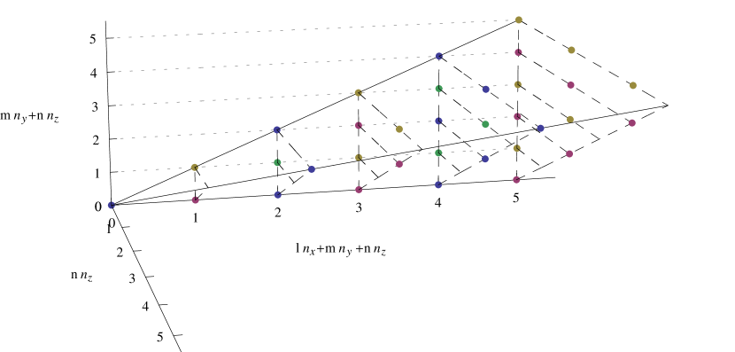
Figure 7: Energy levels for the frequency ratio $1:1:2$. Objects belong to different sets of ($r_{1},r_{2},r_{3}$) values are shown in different color. For each color, the degeneracies are the dimensions of the irreducible representations of SU(3).

V Summary and Conclusions

The Caged Anisotropic Harmonic Oscillator is a new superintegrable Hamiltonian, namely

$$H=\frac{1}{2}(p_{x}^{2}+p_{y}^{2}+p_{z}^{2})+k(l^{2}x^{2}+m^{2}y^{2}+n^{2}z^{2})+\frac{k_{1}}{x^{2}}+\frac{k_{2}}{y^{2}}+\frac{k_{3}}{z^{2}}.$$ (43)

If the frequency multipliers are integers, then the Hamiltonian is superintegrable. We have found the five isolating integrals for the classical motion in three degrees of freedom. Three of the integrals of motion – the energies in each oscillation – are quadratic in the canonical momenta and arise from separation of the Hamilton-Jacobi equation in rectangular Cartesians. The other two integrals are still polynomial in the momenta, but now of order $2(l+m-1)$ and $2(l+n-1)$ respectively. If $l=m=n=1$, the Hamiltonian becomes the well-studied Smorodinsky-Winternitz system Fr65 (7, 8, 17, 28), and all the integrals are then quadratic and arise from separability of the Hamilton-Jacobi equation.

The system is interesting for at least three reasons. First, from the perspective of integrability, there are still very few systems known with integrals of motion that are polynomials in the momenta of higher order than 2 Hie (29). Systematic searches for Hamiltonian systems with higher order polynomial invariants have been performed, confirming the impression that they are rare Thom (30, 31). Given this sketchy and disparate information, we have no unifying theory of the conditions for the existence of such integrals of motion

Second, from the perspective of superintegrability, if the integrals of motion are all quadratic in the momenta, then a classification theorem exists and all systems in flat space have been found Fr65 (7, 8, 9). Such systems always arise from separability of the Hamilton-Jacobi equation in more than one coordinate system. However, the Caged Anisotropic Oscillator joins the Toda Lattice and the Generalized Kepler Problem as an example of a system for which some of the integrals are cubic polynomials or higher, and then the superintegrability does not arise from separability in more than one coordinate system. It would be interesting to classify such systems and find all examples in flat space. In particular, the Caged Anisotropic Oscillator is the second superintegrable Hamiltonian to be deduced by the method of projection introduced in VE08 (15). Essentially, the idea is to view superintegrable motion in three degrees of freedom as a projection of a higher dimensional superintegrable system, such as the Coulomb or Kepler problem, or the harmonic oscillator. Are there any more such systems to be found?

Third, from the perspective of group theory in quantum mechanics, the proper interpretation of the symmetry or degeneracy group remains unclear. Already in 1940, Jauch & Hill Ja40 (10) noted that the quantum mechanical problem of the anisotropic oscillator presents problems which leaves its symmetry group in doubt. Since that day, there have been a number of different suggestions in the literature as to the proper interpretation of the symmetry group Lo73 (24, 25, 26, 27). Although these procedure seem reasonable, they are more along the lines of a posteriori justification than compelling argument.

References

• (1) Pauli W., 1926, Z. Phys., 36, 336
• (2) Fock V., 1935, Z. Phys., 98, 145
• (3) Bargmann V., 1936, Z. Phys., 99, 576
• (4) Abarbanel, H., 1976, in β€œStudies in Mathematical Physics: Essays in Honour of Valentine Bargmann”, eds E.H. Lieb, B. Simon, A.S. Wightman, Princeton, University Press, Princeton, p. 3
• (5) Weigert, S. Thomas H., 1993, Am J. Phys., 61, 272
• (6) Tempesta P., Winternitz P., Harnad J., Miller Jr, W., Pogosyan G., Rodriguez M., 2005, Superintegrability in Classical and Quantum Systems, American Mathematical Society
• (7) Fris J., Mandrosov V., Smorodinsky Y.Β A., UhlΓ­ M., & Winternitz P.Β 1965, Physics Letters, 16, 35
• (8) Makarov A. A., Smorodinsky Y.Β A., Valiev K., & Winternitz P., Β 1967 Nuovo Cimento 52, 1061.
• (9) Evans N.Β W.Β 1990, Phys. Rev. A, 41, 5666
• (10) Jauch J.Β M., & Hill E.Β L.Β 1940, Phys Rev, 57, 641
• (11) Amiet J.-P., & Weigert S.Β 2002, Journal of Math. Phys, 43, 4110
• (12) Boccaletti D., & Pucacco G.Β 1996, Theory of Orbits. Volume 1: Integrable Systems and Non-perturbative Methods, Springer Verlag, New York
• (13) Adler M., 1977, Comm. Math. Phys., 55, 195
• (14) Wojciechowski, S.Β 1983, Physics Letters A, 95, 279
• (15) Verrier P.Β E., & Evans N.Β W.Β 2008, Journal of Math. Phys, 49, 2902
• (16) Evans N.Β W.Β 1991, Journal of Math Phys, 32, 3369
• (17) Ballasteros A., Herranz F.J., 2007, Journal of Phys A: Math Gen, 40, 51
• (18) ErdΓ©lyi A., Magnus W., Oberhettinger F., Tricomi F.G., 1953, Higher Transcendtal Functions vol 2, McGraw-Hill, New York
• (19) Rodriguez M., Tempesta P., Winternitz P. 2008, ArXiv e-prints, 807, arXiv:0807.1047
• (20) Press W.Β H., Teukolsky S.Β A., Vetterling W.Β T., & Flannery B.Β P.Β 2002, Numerical recipes in C++ : the art of scientific computing, Cambridge University Press
• (21) Symon K.R. Β 1960, Mechanics, Addison-Wesley, Reading, Massachusetts, Section 3.10
• (22) Winternitz P., Smorodinsky Ya., Uhlir M., Fris I., 1967, Sov J Nucl Phys 4, 444
• (23) Demkov Yu. N., 1963, Soviet Phys.JETP 17, 1349
• (24) Louck J.Β D., Moshinsky M., Wolf K.Β B.Β 1973, Journal of Math Phys, 14, 692
• (25) King G.Β M.Β 1973, Journal of Phys A: Math Gen, 6, 901
• (26) Rosensteel, G., & Draayer, J.Β P.Β 1989, Journal of Physics A : Math Gen, 22, 1323
• (27) Bonatsos, D., Kolokotronis, P., Lenis, D., & Daskaloyannis, C.Β 1997, Int J of Modern Physics A, 12, 3335
• (28) Evans N.W., 1990, Phys. Lett. A., 147, 483
• (29) Hietarinta J.,1987, Phys Reports, 147, 87
• (30) Thompson G, 1984, Journal of Math Phys, 25, 3474
• (31) Evans N.W, 1990, Journal of Math Phys, 31, 600