A growing dynamo from a saturated Roberts flow dynamo

Abstract

Using direct simulations, weakly nonlinear theory and nonlinear mean-field theory, it is shown that the quenched velocity field of a saturated nonlinear dynamo can itself act as a kinematic dynamo. The flow is driven by a forcing function that would produce a Roberts flow in the absence of a magnetic field. This result confirms an analogous finding by F. Cattaneo & S. M. Tobias (arXiv:0809.1801) for the more complicated case of turbulent convection, suggesting that this may be a common property of nonlinear dynamos; see also the talk given also online at the Kavli Institute for Theoretical Physics (http://online.kitp.ucsb.edu/online/dynamo_c08/cattaneo). It is argued that this property can be used to test nonlinear mean-field dynamo theories.

1 Introduction

The magnetic fields of many astrophysical bodies displays order on scales large compared with the scale of the turbulent fluid motions that are believed to generate these fields via dynamo action. A leading theory for these types of dynamos is mean-field electrodynamics (Moffatt, 1978; Krause & Rädler, 1980), which predicts the evolution of suitably averaged mean magnetic fields. Central to this theory is the mean electromotive force based on the fluctuations of velocity and magnetic fields. This mean electromotive force is then expressed in terms of the mean magnetic field and its first derivative with coefficients $\alpha_{ij}$ and $\eta_{ijk}$. The former represents the $\alpha$ effect and the latter the turbulent magnetic diffusivity.

Under certain restrictions the coefficients $\alpha_{ij}$ and $\eta_{ijk}$ can be calculated using for example the first order smoothing approximation, which means that nonlinearities in the evolution equations for the fluctuations are neglected. Whilst this is a valid approach for small magnetic Reynolds numbers or short correlation times, it is not well justified in the astrophysically interesting case when the magnetic Reynolds number is large and the correlation time comparable with the turnover time. However, in recent years it has become possible to calculate $\alpha_{ij}$ and $\eta_{ijk}$ using the so-called test-field method (Schrinner et al., 2005, 2007). For the purpose of this paper we can consider this method essentially as a “black box” whose input is the velocity field and its output are the coefficients $\alpha_{ij}$ and $\eta_{ijk}$. This method has been successfully applied to the kinematic case of weak magnetic fields in the presence of homogeneous turbulence either without shear (Sur et al., 2008; Brandenburg, Rädler & Schrinner, 2008) or with shear (Brandenburg, 2005; Brandenburg et al., 2008a).

More recently, this method has also been applied to the nonlinear case where the velocity field is modified by the Lorentz force associated with the dynamo-generated field (Brandenburg et al., 2008b) In that case the test-field method consists still of the same black box, whose input is only the velocity field, but now this velocity field is based on a solution of the full hydromagnetic equations comprising the continuity, momentum, and induction equations. We emphasize that the magnetic field is quite independent of the fields that appear in the test-field method inside the black box.

Our present work is stimulated by an interesting and relevant numerical experiment performed recently by Cattaneo & Tobias (2008). They considered a solution of the full hydromagnetic equations where the magnetic field is generated by turbulent convective dynamo action and has saturated at a statistically steady value. They then used this velocity field and subjected it to an independent induction equation, which is equal to the original induction equation except that the magnetic field $\bm{{{B}}}$ is now replaced by a passive vector field $\tilde{\bm{{{B}}}}$, which does not react back on the momentum equation. Surprisingly, they found that $|\tilde{\bm{{{B}}}}|$ grows exponentially, even though the velocity field is already quenched by the original magnetic field.

One might have expected that, because the velocity is modified such that it produces a statistically steady solution to the original induction equation, $\tilde{\bm{{{B}}}}$ should decay or also display statistically steady behavior. The argument sounds particularly convincing for time-independent flows because, if a growing $\tilde{\bm{{{B}}}}$ were to exist, one would expect this alternative field to grow and replace the initial field. This view is supported by recent simulations in which the flow field from a geodynamo simulation in a spherical shell was used as velocity field in kinematic dynamo computations, and no growing $\tilde{\bm{{{B}}}}$ was found (Tilgner, 2008). However, it turns out that this reasoning is not correct in general. One finds counterexamples even within the confines of mean field MHD using analytical tools. The existence of a growing $\tilde{\bm{{{B}}}}$ thus is not tied to chaotic flows or fluctuating small-scale dynamos.

This finding of Cattaneo & Tobias (2008) is interesting in view of the applicability of the test-field method to the nonlinear case. Of course, the equations used in the test-field method are different from the original induction equation. (The equations used in the test-field method include an inhomogeneous term and the mean electromotive force is subtracted, but they are otherwise similar to the original induction equation.) Given the seemingly unphysical behaviour of the induction equation in the presence of a vector field different from the actual magnetic field, it would be tempting to argue that one should choose test fields whose shape is rather close to that of the actual magnetic field (Cattaneo & Hughes, 2008). On the other hand, the $\alpha_{ij}$ and $\eta_{ijk}$ tensors should give the correct response to all possible fields, not just the $\bm{{{B}}}$ field that grew out of a particular initial condition, but also the passive $\tilde{\bm{{{B}}}}$ field that obeys a separate induction equation. It is therefore important to choose a set of test fields that are orthogonal to each other, even if none of the fields are solutions of the induction equation. One goal of this paper is to show that the $\alpha_{ij}$ and $\eta_{ijk}$ tensors obtained in this way provide not only interesting diagnostics of the flow, but they are also able to explain the surprising result of Cattaneo & Tobias (2008) in the context of a simpler example. However, let us begin by repeating the numerical experiment of Cattaneo & Tobias (2008) using the simpler case of a Roberts flow. Next, we consider a weakly nonlinear analysis of this problem and turn then to its mean-field description.

2 The model

In order to examine the possibility of a growing passive vector field, we first considered the case of a driven ABC flow. Such a flow is non-integrable and has chaotic streamlines. Growing passive vector fields were found. To simplify matters even further, we consider now the case of a Roberts flow, which is integrable, has non-chaotic streamlines, and the dynamo can only be a slow one, i.e. the growth rate goes to zero in the limit of large magnetic Reynolds number. This is however not an issue here, because we will only be considering finite values of the magnetic Reynolds number.

In the following we consider both incompressible and isothermal cases. The governing equations for any externally driven velocity field (turbulence, ABC flow, or Roberts flow) are then given by

$${\partial\bm{{{U}}}\over\partial t}=-\bm{{{U}}}\cdot\bm{\nabla}\bm{{{U}}}-\bm{\nabla}H+{1\over\rho}\bm{{{J}}}\times\bm{{{B}}}+\bm{{{f}}}+\bm{{{F}}}_{\rm visc},$$ (1)

$${\partial\bm{{{B}}}\over\partial t}=\bm{\nabla}\times(\bm{{{U}}}\times\bm{{{B}}})+\eta\nabla^{2}\bm{{{B}}},$$ (2)

where $\bm{{{U}}}$ is the velocity, $\bm{{{B}}}$ is the magnetic field, $\rho$ is the density, $H$ is the specific enthalpy, $\bm{{{J}}}=\bm{\nabla}\times\bm{{{B}}}/\mu_{0}$ is the current density, $\mu_{0}$ is the vacuum permeability, $\bm{{{f}}}$ is the forcing function, $\bm{{{F}}}_{\rm visc}$ is the viscous force per unit mass, and $\eta={\rm const}$ is the magnetic diffusivity. In the incompressible case, $\bm{\nabla}\cdot\bm{{{U}}}=0$, we have $H=p/\rho$, where $p$ is the pressure and $\rho={\rm const}$. The viscous force is then given by $\bm{{{F}}}_{\rm visc}=\nu\nabla^{2}\bm{{{U}}}$. In the isothermal case, the density obeys the usual continuity equation

$${\partial\rho\over\partial t}=-\bm{\nabla}\cdot(\rho\bm{{{U}}}),$$ (3)

but now $p=c_{\rm s}^{2}\rho$, where $c_{\rm s}$ is the isothermal sound speed. In that case $H=c_{\rm s}^{2}\ln\rho$ and the viscous force is given by

$$\bm{{{F}}}_{\rm visc}=\nu\nabla^{2}\bm{{{U}}}+{\textstyle{1\over 3}}\nu\bm{\nabla}\bm{\nabla}\cdot\bm{{{U}}}+2\nu\mbox{\boldmath${\sf S}$}{}\bm{\nabla}\ln(\rho\nu),$$ (4)

where ${\sf S}_{ij}={\textstyle{1\over 2}}(U_{i,j}+U_{j,i})-{\textstyle{1\over 3}}\delta_{ij}\bm{\nabla}\cdot\bm{{{U}}}$ is the traceless rate of strain matrix.

In order to compute the evolution of an additional passive vector field $\tilde{\bm{{{B}}}}$ we also solve the equation

$${\partial\tilde{\bm{{{B}}}}\over\partial t}=\bm{\nabla}\times(\bm{{{U}}}\times\tilde{\bm{{{B}}}})+\eta\nabla^{2}\tilde{\bm{{{B}}}}.$$ (5)

In the case of the Roberts flow we use the forcing function

$$\bm{{{f}}}=\nu k_{\rm f}^{2}\bm{{{U}}}_{\rm Rob},$$ (6)

where

$$\bm{{{U}}}_{\rm Rob}=k_{\rm f}\psi\hat{\bm{z}}-\hat{\bm{z}}\times\bm{\nabla}\psi$$ (7)

with

$$\psi=(u_{0}/k_{0})\cos k_{0}x\cos k_{0}y$$ (8)

and $k_{\rm f}=\sqrt{2}k_{0}$. We consider a domain of size $L_{x}\times L_{y}\times L_{z}$. In all cases we consider $L_{x}=L_{y}=L_{z}=2\pi/k_{0}$. Our model is characterized by the choice of fluid and magnetic Reynolds numbers that are here based on the inverse wavenumber $k_{0}$,

$$\mbox{\rm Re}=u_{0}/\nu k_{0},\quad R_{\mathrm{m}}=u_{0}/\eta k_{0}.$$ (9)

3 Numerical experiments

We solve equations (1)–(5) for the isothermal case using the Pencil Code, which is a high-order public domain code (sixth order in space and third order in time) for solving partial differential equations. Equation (5) is solved using the test-field module with the input parameters lignore_uxbtestm=T, and itestfield=’B=0’, which means that the inhomogeneous term of the test-field equation is set to zero and the subtraction of the mean electromotive force has been disabled. In this way we solve equation (5), instead of the original test-field equation. We focus on the case of small fluid Reynolds number, $\mbox{\rm Re}=0.5$. The initial conditions for $\bm{{{B}}}$ and $\tilde{\bm{{{B}}}}$ are Beltrami fields, $(\cos(k_{0}z+\varphi),\sin(k_{0}z+\varphi),0)$, with an arbitrarily chosen phase $\varphi=0.2$, but for $\tilde{\bm{{{B}}}}$ we $\varphi=0$. In Fig. 1 we plot the evolution of the rms values of $\bm{{{B}}}$ and $\tilde{\bm{{{B}}}}$ for a weakly supercritical case with $R_{\mathrm{m}}=6.25$. (In our case with $\mbox{\rm Re}=0.5$ the critical value for dynamo action is $R_{\mathrm{m}}\approx 5.77$; for $\mbox{\rm Re}\to 0$ the critical value would be $R_{\mathrm{m}}\approx 5.5$.) Both $\bm{{{B}}}$ and $\tilde{\bm{{{B}}}}$ grow at first exponentially at the same rate. However, when $\bm{{{B}}}$ reaches saturation, the growth of $\tilde{\bm{{{B}}}}$ slows down temporarily, but then resumes to nearly its original value. This confirms the result of Cattaneo & Tobias (2008) for the much simpler case of a Roberts flow.

Figure 1: Evolution of the rms values of $\bm{{{B}}}$ and $\tilde{\bm{{{B}}}}$ for $R_{\mathrm{m}}=6.25$. The growth rate of $\tilde{\bm{{{B}}}}$ is $0.016\,u_{0}k_{0}$ in the kinematic phase and $0.014\,u_{0}k_{0}$ in the nonlinear phase.

In Fig. 2 we compare horizontal cross-sections of the two fields. Note that the two are phase shifted in the $z$ direction by a quarter wavelength. The short interval in Fig. 1 during which the growth of $\tilde{\bm{{{B}}}}$ slowed down temporarily is therefore related to the fact that the solution needed to “adjust” to this particular form.

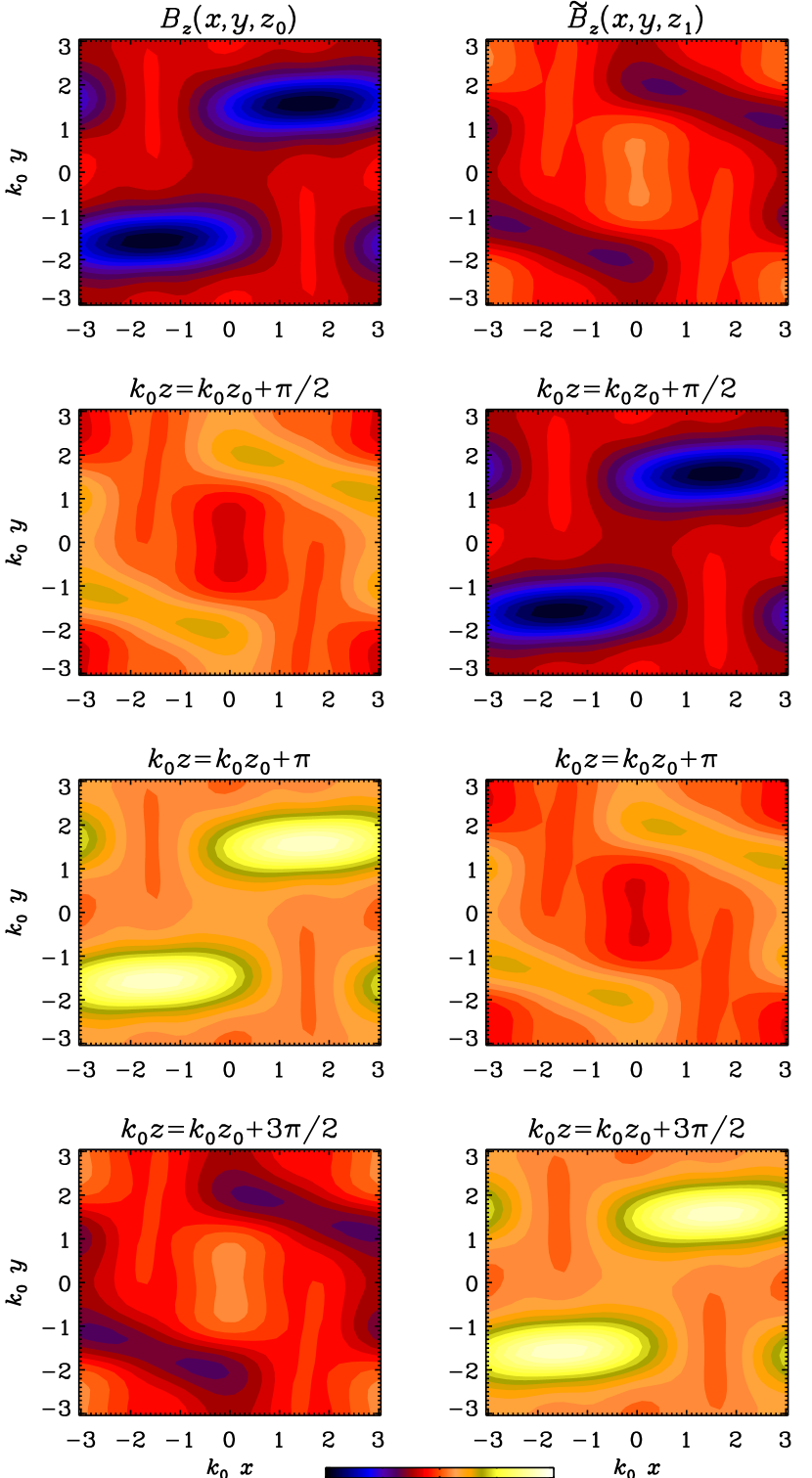
Figure 2: Grey-scale representations of horizontal cross-sections of $\bm{{{B}}}$ and $\tilde{\bm{{{B}}}}$ for $R_{\mathrm{m}}=6.25$. Here, $k_{0}z_{0}\approx-3.04$. Both fields are scaled symmetrically around zero (grey shade) with dark shades indicating negative values and light shades indicating positive vales, as indicated on the greyscale bar.

4 Weakly nonlinear theory

A weakly nonlinear analysis of the Roberts flow is presented in Tilgner & Busse (2001). Two nonlinear terms enter the full dynamo problem. In order to make the calculation analytically tractable, it is assumed that the fluid has infinite magnetic Prandtl number so that the inertial terms (and hence the advection term) drop from the Navier-Stokes equation. The second nonlinear term, the Lorentz force, is assumed to be small compared with the driving force $\bm{{{f}}}$ and is treated perturbatively. The linear induction equation is transformed into a mean field equation assuming separation of length scales and small magnetic Reynolds numbers. One can under these assumptions compute the modifications of the velocity field $\bm{{{U}}}_{\rm Rob}$ due to the presence of a mean field $\bm{\overline{{B}}}$, which we define here as

$$\bm{\overline{{B}}}(z,t)=\int_{0}^{L_{y}}\int_{0}^{L_{x}}\bm{{{B}}}(x,y,z,t)\,\mbox{d}x\,\mbox{d}y/L_{x}L_{y}.$$ (10)

The magnetically modified velocity field then becomes

$$\bm{{{U}}}=(1-\gamma)\bm{{{U}}}_{\rm Rob}+2\gamma\frac{\overline{{B}}_{x}\overline{{B}}_{y}}{\overline{{B}}_{x}^{2}+\overline{{B}}_{y}^{2}}\hat{\bm{{{U}}}}$$ (11)

with

$$\hat{\bm{{{U}}}}=u_{0}\pmatrix{\sin k_{0}x\cos k_{0}y\cr-\cos k_{0}x\sin k_{0}y\cr\sqrt{2}\sin k_{0}x\sin k_{0}y}$$ (12)

and $\gamma=(\overline{{B}}_{x}^{2}+\overline{{B}}_{y}^{2})/(2\eta\nu k_{\rm f}^{2}\rho\mu_{0})$. The original flow $\bm{{{U}}}_{\rm Rob}$ is reduced in magnitude and another 2D periodic flow component is added. The mean-field induction equation with flow $\bm{{{U}}}$ given by (11), written for a passive vector field $\tilde{\bm{{{B}}}}$, is:

$$\frac{\partial\tilde{\bm{{{B}}}}}{\partial t}+\bm{\nabla}\times A\pmatrix{\tilde{B}_{x}\cr\tilde{B}_{y}\cr 0}-\bm{\nabla}\times C\overline{{B}}_{x}\overline{{B}}_{y}\pmatrix{\tilde{B}_{y}\cr\tilde{B}_{x}\cr 0}=\eta\bm{\nabla}^{2}\tilde{\bm{{{B}}}}$$ (13)

with

$$A=\tilde{R}_{\rm m}v_{0}\quad\mbox{and}\quad C={\tilde{R}_{\rm m}^{3}\over P_{\rm m}}{1\over v_{0}\rho\mu_{0}},$$ (14)

where

$$\tilde{R}_{\rm m}={v_{0}\over\eta k_{\rm f}},\quad P_{\rm m}={\nu\over\eta},\quad\mbox{and}\quad v_{0}^{2}={\textstyle{1\over 2}}u_{0}^{2}(1-\gamma)$$ (15)

have been introduced. This equation corresponds to equation (10) of Tilgner & Busse (2001). Apart from a change of notation, the distinction between the passive vector field $\tilde{\bm{{{B}}}}$ and the field distorting the Roberts flow, $\bm{\overline{{B}}}$, has been made. In addition, equation (10) of Tilgner & Busse (2001) was intended as a model of the Karlsruhe dynamo and used $u_{0}$ as control parameter, whereas here, we consider $\bm{{{f}}}$ as given. For this reason, the two equations are identical only to first order in $\gamma$.

Equation (13) reduces to the usual dynamo problem for $\tilde{\bm{{{B}}}}=\bm{\overline{{B}}}$ and leads to the kinematic dynamo problem if it is furthermore linearized in $\bm{\overline{{B}}}$, which corresponds to dropping the third term in Eq. (13). For $u_{0}^{2}>2\eta^{2}k_{\rm f}k$, the equation has growing solutions of the form $(\cos kz,\sin kz,0)$. Weakly nonlinear analysis determines the amplitude $B_{0}$ of a saturated solution of the form $\bm{\overline{{B}}}=B_{0}(\cos kz,\sin kz,0)$ by inserting this ansatz for $\bm{\overline{{B}}}$ and $\tilde{\bm{{{B}}}}=\bm{\overline{{B}}}$ into equation (13) and by projecting equation (13) onto $(\cos kz,\sin kz,0)$ and integrating spatially over a periodicity cell (Tilgner & Busse, 2001).

We proceed similarly to find growing solutions of equation (13). Assume $\bm{\overline{{B}}}=B_{0}(\cos kz,\sin kz,0)$. Obvious candidates for passive vector fields growing at rate $p$ are $\tilde{\bm{{{B}}}}\propto e^{pt}(\cos(kz+\varphi),\sin(kz+\varphi),0)$. Since the third term in equation (13) is a perturbation, a growing solution must be of a form such that the other terms maximize the growth rate. These other terms are identical to the kinematic problem, so that $\tilde{\bm{{{B}}}}$ must have the same general form as the kinematic dynamo field except for the phase shift $\varphi$ which measures the phase angle between the saturated field $\bm{\overline{{B}}}$ and the passive vector field $\tilde{\bm{{{B}}}}$. The velocity field $\bm{{{U}}}_{\rm Rob}$ is independent of $z$, so that any solution of the kinematic dynamo problem remains a solution after translation along $z$. However, neither the Lorentz force due to $\bm{\overline{{B}}}$ nor the flow modified by that Lorentz force are independent of $z$, so that the phase angle $\varphi$ matters for $\tilde{\bm{{{B}}}}$. The above ansatz for $\tilde{\bm{{{B}}}}$ will not be an exact solution of equation (13) because of the $z$-dependence of $\overline{{B}}_{x}\overline{{B}}_{y}$, but it represents the leading Fourier component. In order to determine the optimal $\varphi$, we insert this ansatz into equation (13), project onto $(\cos(kz+\varphi),\sin(kz+\varphi),0)$ and integrate over a periodicity cell to find

$$p=-\eta k^{2}+Ak-CB_{0}^{2}k\frac{1}{4}\cos 2\varphi.$$ (16)

The saturation amplitude $B_{0}$ is determined from this equation by setting $p=0$ and $\varphi=0$. For any given $B_{0}$, the maximum of $p$ is obtained for $\varphi=\pi/2$. The fastest growing mean passive vector field is thus expected to have the same form as the mean dynamo field except for a translation by a quarter wavelength along the $z$-axis. This is in agreement with the simulation results of Sect. 3.

The weakly nonlinear analysis in summary delineates the following physical picture: As detailed in Tilgner & Busse (2001), the saturated dynamo field modifies the flow in two different ways. Firstly, it reduces the amplitude of $\bm{{{U}}}_{\rm Rob}$ by the factor $1-\gamma$, and secondly, it introduces a new set of vortices which lead to the third term in equation (13). The reduction of the amplitude of the Roberts flow affects all magnetic mean fields with a spatial dependence in $(\cos(kz+\varphi),\sin(kz+\varphi),0)$ in the same manner, independently of $\varphi$. The additional vortices, however, have a quenching effect on the field that created them (e.g. $\varphi=0$) but are amplifying for a field shifted by $\varphi=\pi/2$ with respect to the saturated field.

We were able to find a simple growing passive vector field thanks to the periodic boundary conditions in $z$. The same construction is impossible for vacuum boundaries at $z=0$ and $z=2\pi/k_{0}$. Numerical simulations of the Roberts dynamo with vacuum boundaries, not reported in detail here, have revealed that growing $\tilde{\bm{{{B}}}}$ exist in this geometry nonetheless, but they bear a more complicated relation with $\bm{{{B}}}$ than a simple translation. At present, the flow of the convection driven dynamo in a spherical shell used in Tilgner (2008) seems to be the only known example of a dynamo which does not allow for growing $\tilde{\bm{{{B}}}}$.

5 Nonlinear mean-field theory

In mean-field dynamo theory for a flow such as the Roberts flow one solves an equation for the horizontally averaged mean field, as defined in equation (10). The mean electromotive force is defined as $\overline{\mbox{\boldmath${\mathcal{E}}$}}{}=\overline{\bm{{{u}}}\times\bm{{{b}}}}$, where $\bm{{{u}}}=\bm{{{U}}}-\bm{\overline{{U}}}$ and $\bm{{{b}}}=\bm{{{B}}}-\bm{\overline{{B}}}$ are the fluctuating components of magnetic and velocity fields. The mean electromotive force can be expressed in terms of the mean fields as

$${\cal E}_{i}=\alpha_{ij}\overline{{B}}_{j}-\eta_{ij}\overline{{J}}_{j},$$ (17)

where we have used the fact that for mean fields that depend only on one spatial coordinate one can express all first derivatives of the components of $\bm{\overline{{B}}}$ in terms of those of $\bm{\overline{{J}}}$ alone.

The tensorial forms of $\alpha_{ij}$ and $\eta_{ij}$ are ignored in many mean-field dynamo applications, but here their tensorial forms turn out to be of crucial importance. Of course, there is always the anisotropy with respect to the $z$ direction, but this is unimportant in our one-dimensional mean field problem, because of solenoidality of $\bm{\overline{{B}}}$ and $\bm{\overline{{J}}}$ and suitable initial conditions on $\bm{\overline{{B}}}$ such that $\overline{{B}}_{z}=\overline{{J}}_{z}=0$. However, the dynamo-generated magnetic fields will introduce an anisotropy in the $x$ and $y$ directions. If $\bm{\overline{{B}}}$ is the only vector giving a preferred direction to the system, the $\alpha_{ij}$ and $\eta_{ij}$ tensors must be of the form

$$\alpha_{ij}=\alpha_{1}(\bm{\overline{{B}}})\delta_{ij}+\alpha_{2}(\bm{\overline{{B}}})\hat{B}_{i}\hat{B}_{j}+...,$$ (18)

$$\eta_{ij}=\eta_{1}(\bm{\overline{{B}}})\delta_{ij}+\eta_{2}(\bm{\overline{{B}}})\hat{B}_{i}\hat{B}_{j}+...,$$ (19)

where $\hat{\bm{B}}=\bm{\overline{{B}}}/|\bm{\overline{{B}}}|$ is the unit vector of the dynamo-generated mean magnetic field, and dots indicate the presence of terms related to the anisotropy in the $z$ direction inherent to the Roberts flow. As indicated above, equation (18) is correct without these terms only in the $(x,y)$ plane. However, the terms represented by the dots do not enter the considerations below because we are only interested in fields with $\overline{{B}}_{z}=0$.

In order to predict the evolution of $\tilde{\bm{{{B}}}}$ in the saturated state, we need to know the effect on $\alpha_{ij}$ (and in principle also on $\eta_{ij}$, but $\eta_{2}$ is small; see below). Thus, we now need to know $\bm{\overline{{B}}}$. The mean magnetic field generated by the Roberts flow is a force-free Beltrami field of the form

$$\bm{\overline{{B}}}=(\cos k_{0}z,\sin k_{0}z,0),$$ (20)

so

$$\hat{B}_{i}\hat{B}_{j}=\pmatrix{\cos^{2}k_{0}z&\cos k_{0}z\sin k_{0}z&0\cr\cos k_{0}z\sin k_{0}z&\sin^{2}k_{0}z&0\cr 0&0&0}.$$ (21)

The coefficients $\alpha_{1}$, $\alpha_{2}$, $\eta_{1}$, and $\eta_{2}$ have previously been determined for the case of homogeneous turbulence (Brandenburg et al., 2008b) and it turned out at $\alpha_{1}$ and $\alpha_{2}$ have opposite sign, and that $\eta_{2}$ is negligible. This is also true in the present case, for which we have determined $\alpha_{1}/u_{0}=-0.266$, $\alpha_{2}/u_{0}=+0.022$, $\eta_{1}k_{0}/u_{0}=0.082$, and $\eta_{2}k_{0}/u_{0}=0.002$. The microscopic value of $\eta$ is 0.160, so the steady state condition, $\alpha_{1}+\alpha_{2}+(\eta_{1}+\eta_{2}+\eta)k_{0}=0$, is obeyed. In the kinematic regime we have $\alpha_{1}/u_{0}=-0.254$, $\eta_{1}k_{0}/u_{0}=0.076$, with $\alpha_{2}=\eta_{2}=0$, resulting in a positive growth rate of $0.018\,u_{0}k_{0}$. Thus, even though $\alpha_{1}$ increases in this case, the sum $\alpha_{1}+\alpha_{2}$ is being quenched. This, together with the increase of $\eta_{1}+\eta_{2}$, leads to saturation of $\bm{\overline{{B}}}$.

Returning now to the mean-field problem for $\tilde{\bm{{{B}}}}$, this too will be governed by the same $\alpha_{ij}$ and $\eta_{ij}$ tensors, but now the tensor $\hat{B}_{i}\hat{B}_{j}$ is fixed and independent of $\tilde{\bm{{{B}}}}$. The solution for $\tilde{\bm{{{B}}}}$ will be one that maximizes the growth, so it must experience minimal quenching. Such a solution is given by that eigenvector of $\hat{B}_{i}\hat{B}_{j}$ that minimizes the quenching of $\tilde{\bm{{{B}}}}$. In the case of our Beltrami field (18), the minimizing eigenvector is given by

$$\tilde{\bm{\overline{{B}}}}=(\sin k_{0}z,-\cos k_{0}z,0),$$ (22)

which satisfies $\hat{B}_{i}\hat{B}_{j}\tilde{\overline{{B}}}_{j}=0$. This is indeed the same result that we found both numerically and using weakly nonlinear theory. The growth rate of $\tilde{\bm{{{B}}}}$ is then expected to be $|\alpha_{1}|k_{0}-(\eta_{1}+\eta)k_{0}^{2}=0.024\,u_{0}k_{0}$, which is indeed positive, but it is somewhat bigger than the one seen in Fig. 1.

Let us emphasize once more that by determining the full $\alpha_{ij}$ and $\eta_{ij}$ tensors in the nonlinear case, we have been able to predict the behavior of the passive vector field as well. This adds to the credence of the test-field method in the nonlinear case, and confirms that the test-fields can well be very different from the actual solution.

The considerations above suggest that solutions to the passive vector equation equation (5) can be used to provide an independent test of proposed forms of $\alpha$ quenching. Isotropic formulations of $\alpha$ quenching would not reproduce the growth of a passive vector field, and so such quenching expressions can be ruled out, even though the resulting electromotive force for $\bm{\overline{{B}}}$ would be the same. We suggest therefore that the eigenvalues and eigenvectors of equation (5) with a velocity field from a saturated dynamo can be used to characterize the quenching of dynamo parameters ($\alpha$ effect and turbulent diffusivity) and thereby to test proposed forms of $\alpha$ quenching.

6 Conclusions

The most fundamental question of dynamo theory beyond kinematic dynamo theory is “how do magnetic fields saturate?”. In the simplest picture, the velocity field reorganizes in response to the Lorentz force such that all magnetic fields decay except one which has zero growth rate and which is the one we observe. This picture is already questionable for chaotic dynamos. In a chaotic system, nearby initial conditions lead to exponentially separating time evolutions. If one takes a magnetic field $\bm{{{B}}}$ with (on time average) zero growth rate which is the saturated solution of a chaotic dynamo, and solves the kinematic dynamo problem for a passive vector field $\tilde{\bm{{{B}}}}$ with initial conditions different from $\bm{{{B}}}$, one is prepared to find growing $\tilde{\bm{{{B}}}}$. Examples for growing $\tilde{\bm{{{B}}}}$ in chaotic dynamos have been given by Cattaneo & Tobias (2008).

For a time-independent saturated dynamo, on the other hand, the simple picture seems to be adequate at first. However, we have shown in this paper that growing $\tilde{\bm{{{B}}}}$ also exist in the time-independent Roberts dynamo. The origin of the growing $\tilde{\bm{{{B}}}}$ can in this case be understood with the help of weakly nonlinear theory. The growing $\tilde{\bm{{{B}}}}$ has the same shape as the saturated dynamo field but is translated in space.

What was wrong with the naive intuition invoked above? It was based on a stability argument (the equilibrated magnetic field should be replaced by $\tilde{\bm{{{B}}}}$ if there is a growing $\tilde{\bm{{{B}}}}$). However, the linear stability problem for a solution of the full dynamo equations is different from the kinematic dynamo problem for $\tilde{\bm{{{B}}}}$, because in the latter, the velocity field is fixed. Both problems are closely related eigenvalue problems, but standard mathematical theorems do not provide us with a relation between the spectra of both problems. The numerical computation above gives an example of a stable Roberts dynamo, showing that the linear stability problem for the solution found there has only negative eigenvalues. Solving the same eigenvalue problem with velocity fixed, which is the kinematic problem for $\tilde{\bm{{{B}}}}$, can very well lead to positive eigenvalues, and indeed, it does. The dynamo is therefore only stable because the velocity field is able to adjust to perturbations in the magnetic field. The magnetic field on its own is unstable.

References

- Brandenburg (2005) Brandenburg A. 2005, AN, 326, 787
- Brandenburg, Rädler & Schrinner (2008) Brandenburg A., Rädler K.-H., Schrinner M. 2008, A&A, 482, 739
- Brandenburg et al. (2008a) Brandenburg A., Rädler K.-H., Rheinhardt M., Käpylä P. J. 2008a, ApJ, 676, 740
- Brandenburg et al. (2008b) Brandenburg A., Rädler K.-H., Rheinhardt M., Subramanian K. 2008b, ApJ, 687, L49
- Cattaneo & Tobias (2008) Cattaneo F., Tobias S. M. 2008, J. Fluid Mech., arXiv:0809.1801, see also the talk given at the Kavli Institute for Theoretical Physics on 17 July 2008 on “Large and small-scale dynamo action” (http://online.kitp.ucsb.edu/online/dynamo_c08/cattaneo)
- Cattaneo & Hughes (2008) Cattaneo F., Hughes D. W. 2008, MNRAS, arXiv:0805.2138
- Krause & Rädler (1980) Krause F., Rädler K.-H. 1980, Mean-field magnetohydrodynamics and dynamo theory (Pergamon Press, Oxford)
- Moffatt (1978) Moffatt H. K. 1978, Magnetic field generation in electrically conducting fluids (Cambridge University Press, Cambridge)
- Schrinner et al. (2005) Schrinner M., Rädler K.-H., Schmitt D., Rheinhardt M., Christensen U. 2005, AN, 326, 245
- Schrinner et al. (2007) Schrinner M., Rädler K.-H., Schmitt D., Rheinhardt M., Christensen U. 2007, Geophys. Astrophys. Fluid Dyn., 101, 81
- Sur et al. (2008) Sur S., Brandenburg A., Subramanian K. 2008, MNRAS, 385, L15
- Tilgner & Busse (2001) Tilgner A., Busse F. H., 2001, Saturation mechanism in a model of the Karlsruhe dynamo, in: Dynamo and Dynamics, a Mathematical Challenge, Chossat, P. and Armbruster, D. and Oprea, I. eds., Kluwer
- Tilgner (2008) Tilgner A. 2008, Phys. Rev. Lett., 100, 128501