Histogram-Aware Sorting for Enhanced Word-Aligned Compression in Bitmap Indexes

Abstract

Bitmap indexes must be compressed to reduce input/output costs and minimize CPU usage. To accelerate logical operations (AND, OR, XOR) over bitmaps, we use techniques based on run-length encoding (RLE), such as Word-Aligned Hybrid (WAH) compression. These techniques are sensitive to the order of the rows: a simple lexicographical sort can divide the index size by 9 and make indexes several times faster. We investigate reordering heuristics based on computed attribute-value histograms. Simply permuting the columns of the table based on these histograms can increase the sorting efficiency by 40%.

1 Introduction

Bitmap indexes are among the most commonly used indexes in data warehouses [8, 3]. Without compression, bitmap indexes can be impractically large and slow. Word-Aligned Hybrid (WAH) [25] is a competitive compression technique: compared to LZ77 [5] and Byte-Aligned Bitmap Compression (BBC) [1], WAH indexes can be ten times faster [24].

Run-length encoding (RLE) and similar encoding schemes (BBC and WAH) make it possible to compute logical operations between bitmaps in time proportional to the compressed size of the bitmaps. However, their efficiency depends on the order of the rows. While computing the best ordering is NP-hard [2], simple heuristics such as lexicographical sort are effective.

Pinar et al. [14], Sharma and Goyal [18], and Canahuate et al. [4] used Gray-code row sorting to improve RLE and WAH compression. However, their largest bitmap index could fit uncompressed in RAM on a PC.

We distinguish two types of heuristics for this problem. Heuristics such as lexicographical sort [2] or Gray-code sorting [14] are histogram-oblivious. They ignore the number of attribute values and their frequencies. Other heuristics are histogram-aware. They include column reorganizations and frequency-aware ordering. On larger data sets [2], we had considered histogram-oblivious row-ordering heuristics. Sorting before indexing reduced the total construction time. Our main contribution is an evaluation of practical histogram-aware heuristics to the row ordering problem. Secondary contributions include guidelines about when “unary” bitmap encoding is preferred, and an improvement over the naive bitmap construction algorithm—it is now practical to construct bitmap indexes over tables with hundreds of millions of rows and millions of attribute values.

To further reduce the size of bitmap indexes, we can bin the attribute values [12, 17, 20, 7]. For range queries, different bitmap encodings have different space-performance tradeoffs [5, 6].

2 Bitmap Indexes

We find bitmap indexes in several database systems, apparently beginning with the MODEL 204 engine, commercialized for the IBM 370 in 1972.

The simplest and most common method of bitmap indexing associates a bitmap with every attribute value $v$ of every attribute $a$; the bitmap represents the predicate $a=v$. For a table with $n$ rows (facts) and $c$ columns (attributes/dimensions), each bitmap has length $n$. Initially, all bitmap values are set to 0. For row $j$, we set the $j^{\textrm{th}}$ component of $c$ bitmaps to 1. If the $i^{\textrm{th}}$ attribute has $n_{i}$ possible values, we have $L=\sum_{i=1}^{c}n_{i}$ bitmaps.

Bitmap indexes are fast, because we find rows having a given value $v$ for attribute $a$ by reading only the bitmap corresponding to value $v$ (and not the other bitmaps for attribute $a$), and there is only one bit (or less, with compression) to process for each row. More complex queries are achieved with logical operations (AND, OR, XOR, NOT) over bitmaps and current microprocessor can perform 32 or 64 bitwise operations in a single machine instruction.

For row $j$, exactly one bitmap per column will have its $j^{\textrm{th}}$ entry set to 1. Although the entire index has $nL$ bits, there are only $nc$ 1’s; for many tables, $L\gg c$ and thus on average the table is very sparse. Long (hence compressible) runs of 0’s are expected.

One can also reduce the number of bitmaps for large dimensions. Given $L$ bitmaps, there are $L(L-1)/2$ pairs of bitmaps. So, instead of mapping an attribute value to a single bitmap, we map them to pairs of bitmaps (see Table 1). We refer to this technique as 2-of-$N$ encoding [23]; with it, we can use far fewer bitmaps for large dimensions. For instance, with only 2,000 bitmaps, we can represent an attribute with 2 million distinct values. But the average bitmap density is much higher with 2-of-$N$ encoding, and thus compression may be less effective. More generally, $k$-of-$N$ encoding allows $L$ bitmaps to represent $L\choose k$ distinct values; conversely, using $L=\lceil kn_{i}^{1/k}\rceil$ bitmaps is sufficient to represent $n_{i}$ distinct values. However, searching for a specified value $v$ no longer requires scanning a single bitmap. Instead, the corresponding $k$ bitmaps must be combined with a bitwise AND. There is a tradeoff between index size and the index speed [2].

For small dimensions, using $k$-of-$N$ encoding may fail to reduce the number of bitmaps, but still reduce the performance. We apply the following heuristic. Any column with less than 5 distinct values is limited to 1-of-$N$ encoding (simple or unary bitmap). Any column with less than 21 distinct values, is limited to $k=1,2$, and any column with less than 85 distinct values is limited to $k=1,2,3$.

Table 1: Example of 1-of-N and 2-of-N encoding

Montreal	100000000000000	110000
Paris	010000000000000	101000
Toronto	001000000000000	100100
New York	000100000000000	011000
Berlin	000010000000000	010100

3 Compression

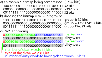
RLE compresses efficiently when there are long runs of identical values: it works by replacing any repetition by the number of repetitions followed by the value being repeated. For example, the sequence 11110000 becomes 4140. Current microprocessors perform operations over words of 32 or 64 bits and not individual bits. Hence, the CPU cost of RLE might be large [19]. By trading some compression for more speed, Antoshenkov [1] defined a RLE variant working over bytes instead of bits: the Byte-Aligned Bitmap Compression (BBC). Trading even more compression for even more speed, Wu et al. [25] proposed the Word-Aligned Hybrid (WAH). Their scheme is made of two different types of words. The first bit of every word distinguishes a verbatim (or dirty) 31-bit word from a running sequence of 31-bit clean words (0x00 or 1x11). Running sequences are stored using 1 bit to distinguish between the type of word (0 for 0x00 and 1 for 1x11) and 30 bits to represent the number of consecutive clean words. Hence, a bitmap of length 62 containing a single 1-bit at position $32$ would be coded as the words 100x01 and 010x00. Because dirty words are stored in units of 31 bits using 32 bits, WAH compression can expand the data by 3%. We created our own WAH variant called Enhanced Word-Aligned Hybrid (EWAH). Contrary to WAH compression, EWAH may never (within 0.1%) generate a compressed bitmap larger than the uncompressed bitmap. It also uses only two types of words (see Fig. 1). The first type is a 32-bit verbatim word. The second type of word is a marker word: the first bit is used to indicate which clean word will follow, 16 bits to store the number of clean words, and 15 bits to store the number of dirty words following the clean words. EWAH bitmaps begin with a marker word.

Figure 1: Enhanced Word-Aligned Hybrid (EWAH)

Given $L$ bitmaps and $n$ rows, we can naively construct a bitmap index in time $O(nL)$ by appending a word to each compressed bitmap every 32 or 64 rows. We found this approach impractically slow when $L$ was large—typically, with $k=1$. Instead, we construct bitmap indexes in time $O(nck+L)=O(nck)$ [2] where $ck$ is the number of true values per row (See Algorithm 1): within each block of 32 rows, we store the values of the bitmaps in a set—omitting any unsolicited bitmap, whose values are all false (0x00). We partition the table horizontally into blocks indexed with compressed bitmaps using a fixed memory budget (256 MiB). Each block of bitmaps is written sequentially and preceded by an array of 4-byte integers containing the location of each bitmap.

  Construct: $B_{1},\ldots,B_{L}$, $L$ compressed bitmaps

  $\omega_{i}\leftarrow 0$ for $1\leq i\leq L$.

  $c\leftarrow 1$ {row counter}

  $\mathcal{N}\leftarrow\emptyset$ {$\mathcal{N}$ records the dirtied bitmaps}

  for each table row do

     for each attribute in the row do

        for each bitmap $i$ corresponding to the attribute value do

           set to true the $(c\bmod w)^{\textrm{th}}$ bit of word $\omega_{i}$

           $\mathcal{N}\leftarrow\mathcal{N}\cup\{i\}$

     if $c$ is a multiple of $w$ then

        for $i$ in $\mathcal{N}$ do

           add $c/w-|B_{i}|-1$ clean words (0x00) to $B_{i}$

           add the word $\omega_{i}$ to bitmap $B_{i}$

           $\omega_{i}\leftarrow 0$

        $\mathcal{N}\leftarrow\emptyset$

     $c\leftarrow c+1$

  for $i$ in {1,2,…,L} do

     add $c/w-|B_{i}|-1$ clean words (0x00) to $B_{i}$

Algorithm 1 Constructing bitmaps. For simplicity, we assume the number of rows is multiple of the word size.

Naively, we could compute logical operations between 2 bitmaps in n/32 bitwise operations. Instead, we compute logical operations (OR, AND, XOR) between 2 bitmaps in time $O(|B_{1}|+|B_{2}|)$ where $|B_{i}|$ is the size of the compressed bitmap [25, 2]. Finally, we can bound the bitmap sizes: $|\bigwedge_{i}B_{i}|\leq\min_{i}|B_{i}|$ and $|\bigvee_{i}B_{i}|\leq\sum_{i}|B_{i}|$.

4 Sorting to Improve Compression

Sorting can benefit bitmap indexes at several levels. We can sort the rows of the table. The sorting order depends itself on the order of the table columns. And finally, we can allocate the bitmaps to the attribute values in sorted order.

4.1 Sorting rows

Reordering the rows of a compressed bitmap index can improve compression. Whether using RLE, BBC, WAH or EWAH, the problem is NP-hard by reduction from the Hamiltonian path problem [2, Theorems 1 and 2]. A simple heuristic begins with an uncompressed index. Rows (binary vectors) are then rearranged to promote runs. In the process, we may also reorder the bitmaps. This is the approach of Canahuate et al. [4], but it uses $\Omega(nL)$ time. For the large dimensions and number of rows we have considered, it is infeasible. A more practical approach [2] is to reorder the table, then construct the compressed index directly; we can also reorder the table columns prior to sorting.

Three types of ordering can be used for ordering rows. We may cluster identical rows, but it is not a competitive heuristic [2].

• In lexicographic order, a sequence $a_{1},a_{2},\ldots$ is smaller than another sequence $b_{1},b_{2},\ldots$ if and only if there is a $j$ such that $a_{j}<b_{j}$ and $a_{i}=b_{i}$ for $i<j$. The Unix sort command provides an efficient mean of sorting flat files into lexicographic order; in under 10 s our test computer (see Section 6) sorted a 5-million-line, 120 MB file. SQL supports lexicographic sort via ORDER BY.

• Gray-code (GC) sorting is defined over bit vectors [14]: the sequence $a_{1},a_{2},\ldots$ is smaller than $b_{1},b_{2},\ldots$ if and only if there exists $j$ such that $a_{j}=a_{1}\oplus a_{2}\oplus\ldots\oplus a_{j-1}$, $b_{j}\not=a_{j}$, and $a_{i}=b_{i}$ for $i<j$. Algorithm 2 shows how to compare sparse GC bit vectors $v_{1}$ and $v_{2}$ in time $O(\min(|v_{1}|,|v_{2}|)$ where $|v_{i}|$ is the number of true value in bit vector $v_{i}$. Sorting the rows of a bitmap index without materializing the uncompressed bitmap index is possible [2]: we implemented an $O(nck\log n)$-time solution for $k$-of-$N$ indexes using an external-memory B-tree [10]. Unfortunately, it proved to be two orders of magnitude slower than lexicographic sort.

  INPUT: arrays $a$ and $b$ representing the position of the ones in two bit vectors

  OUTPUT: whether the bit vector represented by $a$ is less than the one represented by $b$

  $f\leftarrow\texttt{true}$

  $m\leftarrow\min(\textrm{length}(a),\textrm{length}(b))$

  for $p$ in $1,2,\ldots,m$ do

     return $f$ if $a_{p}>b_{p}$ and $\lnot f$ if $a_{p}<b_{p}$

     $f\leftarrow\lnot f$

  return $\lnot f$ if $\textrm{length}(a)>\textrm{length}(b)$, $f$ if $\textrm{length}(b)>\textrm{length}(a)$, and false otherwise

Algorithm 2 Gray-code less comparator between sparse bit vectors

For RLE, the best ordering of the rows of a bitmap index minimizes the sum of the Hamming distances: $\sum_{i}h(r_{i},r_{i+1})$ where $r_{i}$ is the $i^{\textrm{th}}$ row, for $h(x,y)=|\{i|x_{i}\not=y_{i}\}|$. If all $2^{L}$ different rows are present, the GC sort would be an optimal solution to this problem [14]. The following proposition shows that GC sort is also optimal if all ${N\choose k}$ $k$-of-$N$ codes are present. The same is not true of lexicographic order when $k>1$: 0110 immediately follows 1001 among 2-of-4 codes, but their Hamming distance is 4.

Proposition 1

We can enumerate, in GC order, all $k$-of-$N$ codes in time $O(k{N\choose k})$ (optimal complexity). Moreover, the Hamming distance between successive codes is minimal (=2).

Proof.

Let $a$ be an array of size $k$ indicating the positions of the ones in $k$-of-$N$ codes. As the external loop, vary the value $a_{1}$ from 1 to $N-k+1$. Within this loop, vary the value $a_{2}$ from $N-k+2$ down to $a_{1}+1$. Inside this second loop, vary the value of $a_{3}$ from $a_{2}+1$ up to $N-k+3$, and so on. By inspection, we see that all possible codes are generated in increasing GC order. To see that the Hamming distance between successive codes is 2, consider what happens when $a_{i}$ completes a loop. Suppose that $i$ is odd and greater than 1, then $a_{i}$ had value $N-k+i$ and it will take value $a_{i-1}+1$. Meanwhile, by construction, $a_{i+1}$ (if it exists) remains at value $N-k+i+1$ whereas $a_{i+2}$ remains at value $N-k+i+2$ and so on. The argument is similar if $i$ is even.    $\Box$

Figure 2: Probabilities that a bitmap will contain a dirty word, when several ($x$-axis) of 1000 possible attribute values are found in a 32-row chunk. Effects are shown for values with $k$-of-$N$ codes that are adjacent in GC order, adjacent in lexicographic order, or randomly selected.

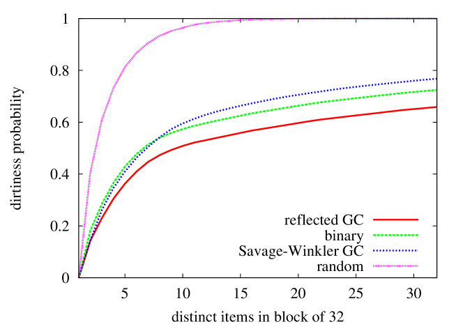
For a given column, suppose that in a block of 32 rows, we have $j$ distinct attribute values. We computed the average number of bitmaps that would have a dirty word (see Fig. 2). Comparing $k$-of-$N$ codes that were adjacent in GC ordering against $k$-of-$N$ codes that were lexicographically adjacent, the difference was insignificant for $k=2$. However, GC ordering is substantially better for $k>2$, where bitmaps are denser. Selecting the codes randomly is disastrous. Hence, sorting part of a column—even one without long runs of identical values—improves compression for $k>1$.

For encodings like BBC, WAH or EWAH, GC sorting is not optimal, even when all $k$-of-$N$ codes are present. For example consider the sequence of rows 1001, 1010, 1100, 0101, 0101, 0110, 0110, 0011. Using 4-bit words, we see that a single bitmap contains a clean word (0000) whereas by exchanging the fifth and second row, we get two clean words (0000 and 1111).

4.2 Sorting bitmap codes

For a simple index, the map from attribute value to bitmaps is inconsequential; for $k$-of-$N$ encodings, some bitmap allocations are more compressible: consider an attribute with two overwhelmingly frequent values and many other values that occur once each. If the table rows are given in random order, the two frequent values should have codes that differ as little as possible.

There are several ways to allocate the bitmaps. Firstly, the attribute values can be visited in alphabetical or numerical order, or—for histogram-aware schemes—in order of frequency. Secondly, the bitmap codes can be used in different orders. We consider lexicographical ordering (1100, 1010, 1001, 0110, …) and GC order (1001, 1010, 1100, 0101, …) ordering (see proof of Proposition 1). For dense low-dimensional tables, GC order is preferable [2] and its compression effects are comparable to sorting the index rows in GC order. Meanwhile, it is technically easier to implement since we can sort the table lexicographically and only use GC ordering during the bitmap index construction.

Alpha-Lex denotes sorting the table lexicographically and assigning bitmap codes so that the $i^{\textrm{th}}$ attribute gets the lexicographically $i^{\textrm{th}}$ smallest bitmap code. Gray-Lex is similar, except that the $i^{\textrm{th}}$ attribute gets the rank-$i$ bitmap code in GC order. These two approaches are histogram oblivious—they ignore the frequencies of attribute values.

Knowing the frequency of each attribute value can improve code assignment when $k>1$. For instance, clustering dirty words increases the compressibility. Within a column, Alpha-Lex and Gray-Lex order runs of identical values irrespective of the frequency: the sequence afcccadeaceabe may become aaaabccccdeeef. For better compression, we should order the attribute values—within a column—by their frequency (e.g., aaaacccceeebdf). Allocating the bitmap codes in GC order to the frequency-sorted attribute values, our Gray-Frequency sorts the table rows as follows. Let $f(a_{i})$ be the frequency of attribute $a_{i}$. Instead of sorting the table rows $a_{1},a_{2},\ldots,a_{d}$, we lexicographically sort the extended rows $f(a_{1}),a_{1},f(a_{2}),a_{2},\ldots,f(a_{d}),a_{d}$ by comparing the frequencies by their numerical value. The frequencies $f(a_{i})$ are discarded prior to indexing.

4.3 Choosing the column order

Lexicographic table sorting uses the $i^{\textrm{th}}$ column as the $i^{\textrm{th}}$ sort key: it uses the first column as the main key, the second column to break ties when two rows have the same first component, and so on. Some column orderings lead to smaller indexes than others [2].

We model the storage cost of a bitmap index as the sum of the number of dirty words and the number of sequences of identical clean words (1x11 or 0x00). If a set of $L$ bitmaps has $x$ dirty words, then there are at most $L+x$ sequences of clean words; the storage cost is at most $2x+L$. This bound will be tighter for sparser bitmaps. Because the simple index of a column has at most $n$ 1-bits, it has at most $n$ dirty words, and thus, the storage cost is at most $3n$. The next proposition shows that the storage cost of a sorted column is bounded by $5n_{i}$.

Proposition 2

Using GC-sorted $k$-of-$L$ codes, a sorted column with $n_{i}$ distinct values has no more than $2n_{i}$ dirty words, and the storage cost is no more than $4n_{i}+\lceil kn_{i}^{1/k}\rceil$.

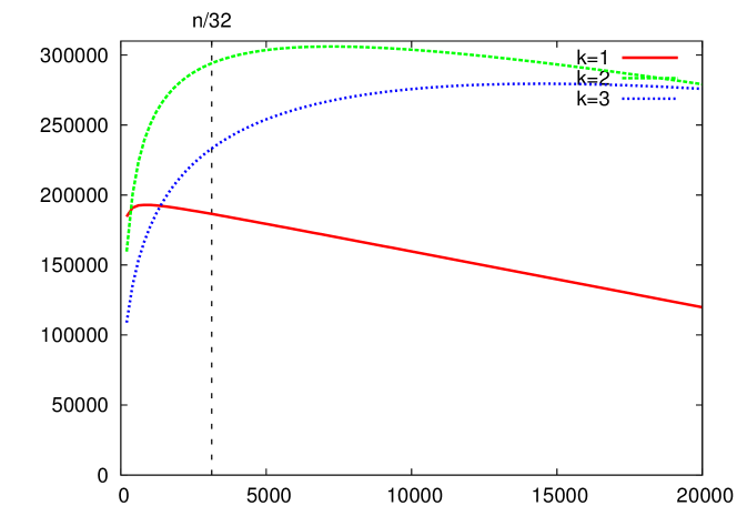
For $k=1$, Proposition 2 is true irrespective of the order of the values, as long as identical values appear sequentially. Another extreme is to assume that all 1-bits are randomly distributed. Then sparse bitmap indexes have $\approx\delta(r,L,n)=(1-(1-\frac{r}{Ln})^{w})\frac{Ln}{w}$ dirty words where $r$ is the number of 1-bits, $L$ is the number of bitmaps and $w$ is the word length ($w=32$). Hence, we have an approximate storage cost of $2\delta+\lceil kn_{i}^{1/k}\rceil$. The gain of column $\mathcal{C}$ is the difference between the expected storage cost of a randomly row-shuffled $\mathcal{C}$, minus the storage cost of a sorted $\mathcal{C}$. We estimate the gain by $2\delta(kn,\lceil kn_{i}^{1/k}\rceil,n)-4n_{i}$ (see Fig. 3) for columns with uniform histograms. The gain is modal: it increases until a maximum is reached and then it decreases. The maximum gain is reached at $\approx\left(n(w-1)/2\right)^{k/(k+1)}$: for $n=100,000$ and $w=32$, the maximum is reached at $\approx 1,200$ for $k=1$ and at $\approx 13,400$ for $k=2$. Skewed histograms have a lesser gain for a fixed cardinality $n_{i}$.

Figure 3: Storage gain in words for sorting a given column with $100,000$ rows and various number of attribute values ($2\delta(kn,\lceil kn_{i}^{1/k}\rceil,n)-4n_{i}$ ).

After lexicographic sorting, the $i^{\textrm{th}}$ column is divided into at most $n_{1}n_{2}\cdots n_{i-1}$ sorted blocks. Hence, it has at most $2n_{1}\cdots n_{i}$ dirty words. When the distributions are skewed, the $i^{\textrm{th}}$ column will have blocks of different lengths and their ordering depends on how the columns are ordered. To assess these effects, we generated data with 4 independent columns: using uniformly distributed dimensions of different sizes (see Fig. 4(a)) and using same-size dimensions of different skew (see Fig. 4(b)). We then determined the Gray-Lex index size for each of the 4! different dimension orderings. Based on these results, for sparse indexes ($k=1$), dimensions should be ordered from least to most skewed, and from smallest to largest; whereas the opposite is true for $k>1$.

(a) Uniform histograms with cardinalities 200, 400, 600, 800

(b) Zipfian data with skew parameters 1.6, 1.2, 0.8 and 0.4

Figure 4: Index sizes in words for various dimension orders on synthetic data ($100,000$ rows). Zipfian columns have 100 distinct values. Ordering “1234” indicates ordering by descending skew (Zipfian) or ascending cardinality (uniform).

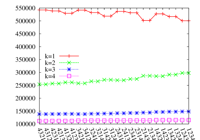
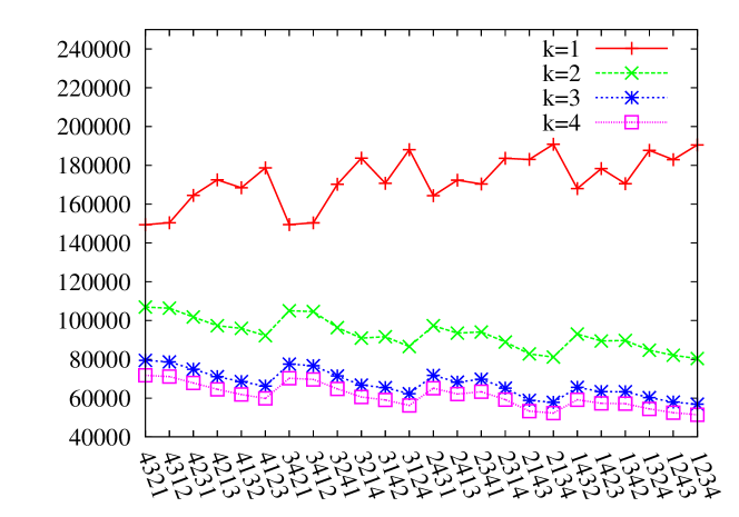
A sensible heuristic might be to sort columns by increasing density ($\approx n_{i}^{-1/k}$). However, a very sparse column ($n_{i}^{1/k}\gg w$) will not benefit from sorting (see Fig. 3) and should be put last. Hence, we use the following heuristic: columns are sorted in decreasing order with respect to $\min(n_{i}^{-1/k},(1-n_{i}^{-1/k})/(4w-1))$: this function is maximum at density $n_{i}^{-1/k}=1/(4w)$ and it goes down to zero as the density goes to 1. In Fig. 4(a), this heuristic makes the best choice for all values of $k$. We consider this heuristic further in Section 6.3.

4.4 Avoiding column order

As an alternative to lexicographic sort and column reordering, we introduce Frequent-Component sorting, which uses histograms to help sort without bias from a fixed dimension ordering. In sorting, we compare the frequency of the $i^{\textrm{th}}$ most frequent attribute values in each of two rows without regard (except for possible tie-breaking) to which columns they come from. With appropriate pre- and post-processing, it is possible to implement this approach using a standard sorting utility such as Unix sort.

5 Picking the Right k-of-N

Choosing $k$ and $N$ are important decisions. We choose a single $k$ value for all dimensions, leaving the possibility of varying $k$ by dimension as future work. Larger values of $k$ typically lead to a smaller index and a faster construction time—although we have observed cases where $k=2$ makes a larger index. However, query times increase with $k$: there is a construction time/speed tradeoff.

Larger $k$ makes queries slower

We can bound the additional cost of queries. Assume ${L_{i}\choose k}=n_{i}$. A given $k$-of-$L_{i}$ bitmap is the result of an OR operation over at most $kn_{i}/L_{i}\leq 3n_{i}^{(k-1)/k}$ unary bitmaps. Because $|\bigvee_{i}B_{i}|\leq\sum_{i}|B_{i}|$, the expected size of such a bitmap is no larger than $3n_{i}^{(k-1)/k}$ times the expected size of a unary bitmap. A query looking for one attribute value will have to AND together $k$ of these denser bitmaps. The entire ANDing operation can be done by $k-1$ pairwise ANDs that produce intermediate results whose EWAH sizes are increasingly small: $2k-1$ bitmaps are thus processed. Hence, the expected time complexity of an equality query on a dimension of size $n_{i}$ is no more than $3(2k-1)n_{i}^{\frac{k-1}{k}}$ times higher than the expected cost of the same query on a $k=1$ index.

For a less pessimistic estimate of this dependence, observe that indexes seldom increase in size when $k$ grows. We may conservatively assume that index size is unchanged when $k$ changes. Therefore the expected size of one bitmap grows as $\approx n_{i}^{-1/k}/k$, leading to queries whose cost is proportional to $(2-1/k)n_{i}^{-1/k}$. Relative to the cost for $k=1$, which is proportional to $1/n_{i}$, we can say that increasing $k$ leads to queries that are$(2-1/k)n_{i}^{(k-1)/k}$ times more expensive than on a simple bitmap index.

For example, suppose $n_{i}=100$, going from $k=1$ to $k=2$ should increase query cost about 15 fold but no more than 90 fold. In summary, the move from $k=1$ to anything larger can have a dramatic negative effect on query speeds. Once we are at $k=2$, the incremental cost of going to $k=3$, $k=4$ is not so high: whereas the ratio $k=2/k=1$ goes as $\sqrt{n_{i}}$, the ratio $k=3/k=2$ goes as $n_{i}^{1/6}$.

Larger $k$ makes indexes smaller

Consider the effect of a length 100 run of values $v_{1}$, followed by 100 repetitions of $v_{2}$, then 100 of $v_{3}$, etc. Regardless of $k$, whenever we switch from $v_{1}$ to $v_{i+1}$ at least two bitmaps will have to make transitions between 0 and 1. Thus, unless the transition appears at a word boundary, we create at least 2 dirty words whenever an attribute changes from row to row. The best case, where only 2 dirty words are created, is achieved when $k=1$ for any assignment of bitmap codes to attribute values. For $k>1$ and $N$ as small as possible, it may not be possible to achieve so few dirty words, or it may require a particular assignment of bitmap codes to values.

Encodings with $k>1$ find their use when many (e.g. 15) attribute values fall within a word-length boundary. In that case, a $k=1$ index will have at least 15 bitmaps with transitions (and we can anticipate 15 dirty words). However, if there were only 45 possible values in the dimension, we would not need more than 10 bitmaps with $k=2$. Hence, there would be at most 10 dirty words and maybe less if we have sorted the data (see Fig. 2).

Choosing $N$

It seems intuitive, having chosen $k$, to choose $N$ to be as small as possible. Yet, we have observed cases where the resulting 2-of-$N$ indexes are much bigger than 1-of-$N$ indexes. Theoretically, this could be avoided if we allowed larger $N$, because one could aways append an additional 1 to every attribute’s 1-of-$N$ code. Since this would create one more (clean) bitmap than the 1-of-$N$ index has, this 2-of-$N$ index would never be much larger than the 1-of-$N$ index. So, if $N$ is unconstrained, we can see that there is never a significant space advantage to choosing $k$ small.

Nevertheless, the main advantage of $k>1$ is fewer bitmaps. We choose $N$ as small as possible.

6 Experimental Results

We present experiments to assess the effects of various factors (choices of $k$, sorting approaches, dimension orderings) in terms of EWAH index sizes. These factors also affect index creation and query times (we report real wall-clock times).

6.1 Platform

Our test programs were written in C++ and compiled by GNU GCC 4.0.2 on an Apple Mac Pro with two double-core Intel Xeon processors (2.66 GHz) and 2 GiB of RAM. Lexicographic sorts of flat files were done using GNU coreutils sort version 6.9. For all tests involving $k=1$, we used the sparse implementation approached in Section 3 because without it, the Gray-Lex index creation times were 20–100 times slower, depending on the data set.

6.2 Data sets used

We primarily used four data sets, whose details are summarized in Table 2: Census-Income [9], DBGEN [21], KJV-4grams, and Netflix [13]. DBGEN is a synthetic data set, whereas KJV-4grams is a large list (including duplicates) of 4-tuples of words obtained from the verses in the King James Bible [16], after stemming with the Porter algorithm [15] and removal of stemmed words with three or fewer letters. Occurrence of row $w_{1},w_{2},w_{3},w_{4}$ indicates that the first paragraph of a verse contains words $w_{1}$ through $w_{4}$, in this order. This data is a scaled-up version of word co-occurrence cubes used to study analogies in natural language [22, 11]. Each of KJV-4grams’ columns contains roughly 8 thousand distinct stemmed words. The Netflix table has 4 dimensions: UserID, MovieID, Date and Rating, having cardinalities 5, 2 182, 17 770, and 480 189. Details of how it was obtained from the data downloaded are given elsewhere [2].

Table 2: Characteristics of data sets used.

	rows	cols	$\sum_{i}n_{i}$	size
Census-Income	199 523	42	103 419	99.1 MB
4-d projection	199 523	4	102 609	2.96 MB
DBGEN	13 977 980	16	4 411 936	1.5 GB
4-d projection	13 977 980	4	402 544	297 MB
Netflix	100 480 507	4	500 146	2.61 GB
KJV-4grams	877 020 839	4	33 553	21.6 GB

For some of our tests, we chose four dimensions with a wide range of sizes. For Census-Income, we chose age ($d_{1}$), wage per hour ($d_{2}$), dividends from stocks ($d_{3}$) and a numerical value found in the $25^{\textrm{th}}$ position ($d_{4}$). Their respective cardinalities were 91, 1 240, 1 478 and 99 800. For DBGEN, we selected dimensions of cardinality 7, 11, 2 526 and 400 000. Dimensions are numbered by increasing size: column 1 has fewer distinct values.

6.3 Column Ordering

Fig. 5 shows the Gray-Lex index sizes for each column ordering. The dimensions of KJV-4grams are too similar for ordering to be interesting, and we have thus omitted them. For small dimensions, the value of $k$ was lowered using the heuristic presented in Section 2. Our results suggest that table-column reordering has a significant effect (40%). This does not contradict the observation by Canahuate et. al [4] that bitmap reordering does not change the size much.

The value of $k$ affects which ordering leads to the smallest index: good orderings for $k=1$ are frequently bad orderings for $k>1$, and vice versa. This is consistent with our earlier analysis (see Figs. 3 and 4). For Netflix and DBGEN, we have omitted $k=2$ for legibility: it is inferior to $k=1$ for most orderings.

(a) Census-Income

(b) DBGEN

(c) Netflix

Figure 5: Index sizes (words, $y$ axis) on 4-d data sets for all dimension orderings ($x$ axis).

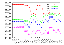
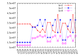
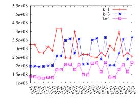
Census-Income’s largest dimension is very large ($n_{4}\approx n/2$); DBGEN has also a large dimension ($n_{4}\approx n/35$). Sorting columns in decreasing order with respect to $\min(n_{i}^{-1/k},(1-n_{i}^{-1/k})/(4w-1))$ for $k=1$, we have that only for DBGEN the ordering “2134” is suggested, otherwise, “1234” is recommended. Thus the heuristic provides nearly optimal recommendations. For $k=3$ and $k=4$, the ordering “1234” is recommended for all data sets: for $k=4$ and Census-Income, this recommendation is wrong. For $k=2$ and Census-Income, the ordering “3214” is recommended, another wrong recommendation for this data set. Hence, a better column reordering heuristic is needed for $k>1$. The difficulty appears to be fundamental: when we calculated the gain experimentally, we found that the best orderings sometimes did not have the dimensions with highest gain first. Our greedy approach may be too simple, and it it may be necessary to know the histogram skews.

6.4 Sorting

On some synthetic Zipfian tests, we found a small improvement (less than 4% for 2 dimensions) by using Gray-Lex coding in preference to Alpha-Lex [2, Fig. 3]. On other data sets, Gray-Lex either had no effect or a small positive effect. Therefore, our current experiments do not include Alpha-Lex, with the exception that we experimentally evaluated how sorting affects the EWAH compression of individual columns. Whereas sorting tends to create runs of identical values in the first columns, the benefits of sorting are far less apparent in later columns, except those strongly correlated with the first few columns. For Table 3, we have sorted projections of Census-Income and DBGEN onto 10 dimensions $d_{1}\ldots{}d_{10}$ with $n_{1}<\ldots<n_{10}$. (The dimensions $d_{1}\ldots d_{4}$ in this group are different from the dimensions $d_{1}\ldots d_{4}$ discussed earlier.) We see that if we sort from the largest column ($d_{10}\ldots{}d_{1}$), at most 3 columns benefit from the sort, whereas 5 or more columns benefit when sorting from the smallest column ($d_{1}\ldots{}d_{10}$).

Table 3: Number of 32-bit words used for different unary indexes when the table was sorted lexicographically (dimensions ordered by descending cardinality, $d_{10}\ldots d_{1}$, or by ascending cardinality, $d_{1}\ldots d_{10}$).

	Census-Income				DBGEN
	cardinality	unsorted	$d_{1}\ldots d_{10}$	$d_{10}\ldots d_{1}$	cardinality	unsorted	$d_{1}\ldots d_{10}$	$d_{10}\ldots d_{1}$
$d_{1}$	7	42 427	32	42 309	2	0.75$\times 10^{6}$	24	0.75$\times 10^{6}$
$d_{2}$	8	36 980	200	36 521	3	1.11$\times 10^{6}$	38	1.11$\times 10^{6}$
$d_{3}$	10	34 257	1 215	28 975	7	2.58$\times 10^{6}$	150	2.78$\times 10^{6}$
$d_{4}$	47	0.13$\times 10^{6}$	12 118	0.13$\times 10^{6}$	9	0.37$\times 10^{6}$	100 6	3.37$\times 10^{6}$
$d_{5}$	51	35 203	17 789	28 803	11	4.11$\times 10^{6}$	10 824	4.11$\times 10^{6}$
$d_{6}$	91	0.27$\times 10^{6}$	75 065	0.25$\times 10^{6}$	50	13.60$\times 10^{6}$	0.44$\times 10^{6}$	1.42$\times 10^{6}$
$d_{7}$	113	12 199	9 217	12 178	2 526	23.69$\times 10^{6}$	22.41$\times 10^{6}$	23.69$\times 10^{6}$
$d_{8}$	132	20 028	14 062	19 917	20 000	24.00$\times 10^{6}$	24.00$\times 10^{6}$	22.12$\times 10^{6}$
$d_{9}$	1 240	29 223	24 313	28 673	400 000	24.84$\times 10^{6}$	24.84$\times 10^{6}$	19.14$\times 10^{6}$
$d_{10}$	99 800	0.50$\times 10^{6}$	0.48$\times 10^{6}$	0.30$\times 10^{6}$	984 297	27.36$\times 10^{6}$	27.31$\times 10^{6}$	0.88$\times 10^{6}$
total	-	1.11$\times 10^{6}$	0.64$\times 10^{6}$	0.87$\times 10^{6}$	-	0.122$\times 10^{9}$	0.099$\times 10^{9}$	$0.079\times 10^{9}$

Lexicographic sorting

Constructing a simple bitmap index (using Gray-Lex) over KJV-4grams took approximately 14,000 seconds or less than four hours. Nearly half (6,000 s) of the time was due to the sort utility, since the data set is much larger than the machine’s main memory (2 GiB). Constructing an unsorted index is faster (approximately 10,000 s), but the index is about 9 times larger.

To study scaling, we built indexes from prefixes of the full data set. We found construction times increased linearly with index size for $k=1$, whether or not sorting was used. For $1\leq k\leq 4$, index size increased linearly with the prefix size for unsorted data. Yet with sorting, index size increased sublinearly. As new data arrives, it is increasingly likely to fit into existing runs, once sorted.

Table 4 shows index sizes for our large data sets, using Gray-Lex orderings and Gray-Frequency. Dimensions were ordered from the largest to the smallest (“4321”) except for Census-Income where we used the ordering “3214”. We observed that KJV-4grams did not benefit in index size for $k=2$. This data set has many very long runs of identical attribute values in the first two dimensions, and the number of attribute values is modest, compared with the number of rows. This is ideal for 1-of-$N$.

Gray-Frequency yields the smallest indexes in Table 4. Frequent-Component is not shown in the table. On Netflix for $k=1$ it outperformed the other approaches by 1%, and for DBGEN it was only slightly worse than the others. But in all other case on DBGEN, Census-Income and Netflix, it lead to indexes 5–50% larger.

Table 4: Sizes of EWAH indexes (32-bit words) for various sorting methods.

		Lex unsorted	Gray-Lex	Gray-Freq
Census-Income	$k=1$	$8.49\times 10^{5}$	$4.87\times 10^{5}$	$4.87\times 10^{5}$
(4d)	2	$9.12\times 10^{5}$	$4.52\times 10^{5}$	$4.36\times 10^{5}$
	3	$6.90\times 10^{5}$	$3.73\times 10^{5}$	$3.28\times 10^{5}$
	4	$4.58\times 10^{5}$	$2.17\times 10^{5}$	$1.98\times 10^{5}$
DBGEN	1	$5.48\times 10^{7}$	$3.38\times 10^{7}$	$3.38\times 10^{7}$
(4d)	2	$7.13\times 10^{7}$	$2.76\times 10^{7}$	$2.74\times 10^{7}$
	3	$5.25\times 10^{7}$	$1.50\times 10^{7}$	$1.50\times 10^{7}$
	4	$3.24\times 10^{7}$	$1.21\times 10^{7}$	$1.19\times 10^{7}$
Netflix	1	$6.20\times 10^{8}$	$3.22\times 10^{8}$	$3.19\times 10^{8}$
	2	$8.27\times 10^{8}$	$3.17\times 10^{8}$	$2.43\times 10^{8}$
	3	$5.73\times 10^{8}$	$1.97\times 10^{8}$	$1.49\times 10^{8}$
	4	$3.42\times 10^{8}$	$1.37\times 10^{8}$	$1.14\times 10^{8}$
KJV-4grams	1	$6.08\times 10^{9}$	$6.68\times 10^{8}$	$6.68\times 10^{8}$
	2	$8.02\times 10^{9}$	$9.93\times 10^{8}$	$7.29\times 10^{8}$
	3	$4.13\times 10^{9}$	$8.31\times 10^{8}$	$5.77\times 10^{8}$
	4	$2.52\times 10^{9}$	$6.39\times 10^{8}$	$5.01\times 10^{8}$

6.5 Queries

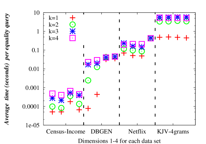
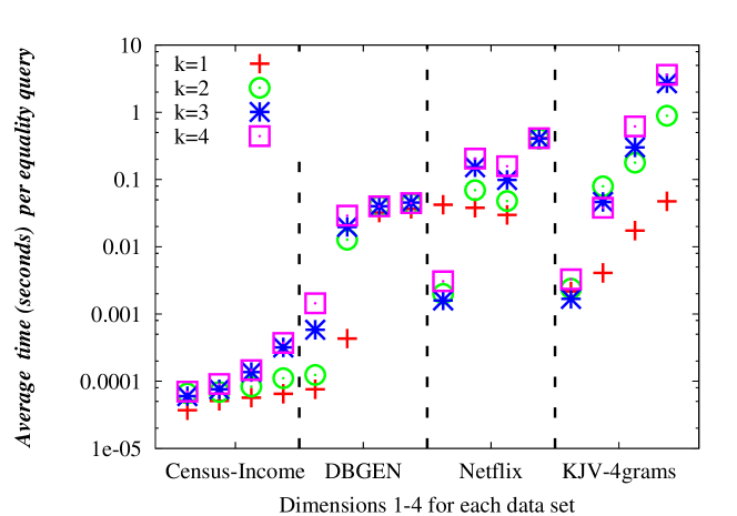
We timed equality queries against our 4-d bitmap indexes, and the results are shown in Fig. 6. Queries were generated by choosing attribute values uniformly at random and the figures report average times for such queries. We made 100 random choices per column for KJV-4grams when $k>1$. For DBGEN and Netflix, we had 1,000 random choices per column and 10,000 random choices were used for Census-Income and KJV-4grams ($k=1$). For each data set, we give the results per column (leftmost tick is the column used as the primary sort key, next tick is for the secondary sort key, etc.).

From Fig. 6(b), we see that simple bitmap indexes always yield the fastest queries. The difference caused by $k$ is highly dependent upon the data set and the particular column in the data set. However, for a given data set and column, with only a few small exceptions, query times increase significantly with $k$. For DBGEN, the last two dimensions have size 7 and 11, whereas for Netflix, the last dimension has size 5, and therefore, they will never use a $k$-value larger than 2: their speed is mostly oblivious to $k$.

In Section 5, we predicted that the query time would grow with $k$ as $\approx(2-1/k)n_{i}^{-1/k}$: for the large dimensions such as the largest ones for DBGEN (400k) and Netflix (480k), query times are two orders of magnitude slower for $k=2$ as opposed to $k=1$, and four orders of magnitude slower for $k=4$. Thus, our model exaggerates the differences by about an order of magnitude. The most plausible explanation is that query times are not directly proportional to the bitmap loaded, but also include a constant factor.

Fig. 6(a) and 6(b) show the equality query times per column before and after sorting the tables. Sorting improves query times most for larger values of $k$: for Netflix, sorting improved the query times by at most 2 for $k=1$, at most 40 for $k=2$ and at most 140 for $k=3$; indexes with $k>1$ benefit from sorting even when there are no long runs of identical values (see Subsection 4.1). (On the first columns, $k=3$ usually gets the best improvements from sorting.) Synthetic DBGEN showed no significant speedup from sorting, beyond its large first column. Although Netflix, like DBGEN, has a many-valued column first, it shows a benefit from sorting even in its third column: in fact, the third column benefits more from sorting than the second column. The largest table, KJV-4grams, benefited most from the sort: while queries on the last column are twice as fast, the gain on the first two columns ranges from 20 times faster ($k=1$) to almost 1500 times faster ($k=3$).

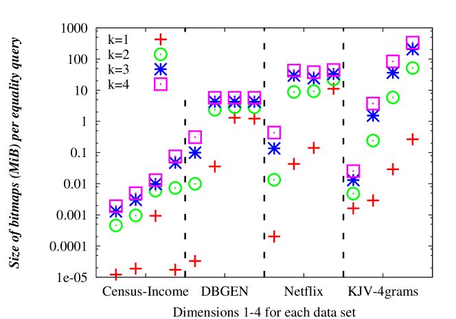
We can compare these times with the expected amount of data scanned per query. This is shown in Figure 7, and we observe reasonably close agreement between most query times and the expected sizes of the bitmaps being scanned. Exceptions include the first dimension on KJV-4grams and some cases where the bitmaps are tiny. This discrepancy might be explained by the retrieval of the row IDs from the compressed bitmaps: long runs of 1x11 clean words must be converted to many row IDs.

(a) Query times over unsorted indexes

(b) Query times over sorted (Gray-Lex) indexes

Figure 6: Query times are affected by dimension, table sorting and $k$.

Figure 7: Bitmap data examined per equality query.

7 Guidelines for k

Our experiments indicate that simple ($k=1$) bitmap encoding is preferable when storage space and index-creation time are less important than fast equality queries. The storage and index-creation penalties are kept modest by table sorting and Algorithm 1.

Space requirements can be reduced by choosing $k>1$, although Tab. 4 shows that this approach has risks (see KJV-4grams). For $k>1$, we can gain additional index size reduction at the cost of longer index construction by using Gray-Frequency rather than Gray-Lex.

If the total number of attribute values is small relative to the number of rows, then we should first try the $k=1$ index. Perhaps the data set resembles KJV-4grams. Besides yielding faster queries, the $k=1$ index may be smaller.

8 Conclusion and Future Work

We showed that while sorting improves bitmap indexes, we can improve them even more (30–40%) if we know the number of distinct values in each column. For $k$-of-$N$ encodings with $k>1$, even further gains (10–30%) are possible using the frequency of each value. Regarding future work, the accurate mathematical modelling of compressed bitmap indexes remains an open problem.

References

- [1] G. Antoshenkov. Byte-aligned bitmap compression. In DCC ’95, page 476, 1995.
- [2] K. Aouiche, D. Lemire, and O. Kaser. Tri de la table de faits et compression des index bitmaps avec alignement sur les mots. available from http://arxiv.org/abs/0805.3339.
- [3] L. Bellatreche, R. Missaoui, H. Necir, and H. Drias. Selection and pruning algorithms for bitmap index selection problem using data mining. LNCS, 4654:221, 2007.
- [4] G. Canahuate, H. Ferhatosmanoglu, and A. Pinar. Improving bitmap index compression by data reorganization. http://hpcrd.lbl.gov/~apinar/papers/TKDE06.pdf (checked 2008-05-30), 2006.
- [5] C. Y. Chan and Y. E. Ioannidis. Bitmap index design and evaluation. In SIGMOD’98, pages 355–366, 1998.
- [6] C. Y. Chan and Y. E. Ioannidis. An efficient bitmap encoding scheme for selection queries. In SIGMOD’99, pages 215–226, 1999.
- [7] R. Darira, K. C. Davis, and J. Grommon-Litton. Heuristic design of property maps. In DOLAP’06, pages 91–98, 2006.
- [8] K. Davis and A. Gupta. Data Warehouses and OLAP: Concepts, Architectures, and Solutions, chapter Indexing in Data Warehouses. IRM Press, 2007.
- [9] S. Hettich and S. D. Bay. The UCI KDD archive. http://kdd.ics.uci.edu (checked 2008-04-28), 2000.
- [10] M. Hirabayashi. QDBM: Quick database manager. http://qdbm.sourceforge.net/ (checked 2008-02-22), 2006.
- [11] O. Kaser, S. Keith, and D. Lemire. The LitOLAP project: Data warehousing with literature. In CaSTA’06, 2006.
- [12] N. Koudas. Space efficient bitmap indexing. In CIKM ’00, pages 194–201, 2000.
- [13] Netflix, Inc. Nexflix prize. http://www.netflixprize.com (checked 2008-04-28), 2007.
- [14] A. Pinar, T. Tao, and H. Ferhatosmanoglu. Compressing bitmap indices by data reorganization. In ICDE’05, pages 310–321, 2005.
- [15] M. F. Porter. An algorithm for suffix stripping. In Readings in information retrieval, pages 313–316. Morgan Kaufmann, 1997.
- [16] Project Gutenberg Literary Archive Foundation. Project Gutenberg. http://www.gutenberg.org/ (checked 2007-05-30), 2007.
- [17] D. Rotem, K. Stockinger, and K. Wu. Minimizing I/O costs of multi-dimensional queries with bitmap indices. In SSDBM ’06, pages 33–44, 2006.
- [18] Y. Sharma and N. Goyal. An efficient multi-component indexing embedded bitmap compression for data reorganization. Information Technology Journal, 7(1):160–164, 2008.
- [19] K. Stockinger, K. Wu, and A. Shoshani. Strategies for processing ad hoc queries on large data warehouses. In DOLAP’02, pages 72–79, 2002.
- [20] K. Stockinger, K. Wu, and A. Shoshani. Evaluation strategies for bitmap indices with binning. In DEXA 2004, 2004.
- [21] TPC. DBGEN 2.4.0. http://www.tpc.org/tpch/ (checked 2007-12-4), 2006.
- [22] P. D. Turney and M. L. Littman. Corpus-based learning of analogies and semantic relations. Machine Learning, 60(1–3):251–278, 2005.
- [23] H. K. T. Wong, H. F. Liu, F. Olken, D. Rotem, and L. Wong. Bit transposed files. In VLDB 85, pages 448–457, 1985.
- [24] K. Wu, E. J. Otoo, and A. Shoshani. A performance comparison of bitmap indexes. In CIKM ’01, pages 559–561, 2001.
- [25] K. Wu, E. J. Otoo, and A. Shoshani. Optimizing bitmap indices with efficient compression. ACM Transactions on Database Systems (TODS), 31(1):1–38, 2006.