Why many theories of shock waves are necessary. Convergence error in formally path-consistent schemes

Manuel J. Castro Departamento de Análisis Matemático, Universidad de Málaga, 29071 Málaga, Spain. Castro@anamat.cie.uma.es Philippe G. LeFloch Laboratoire J.-L. Lions & Centre National de la Recherche Scientifique,
Université de Paris 6, 4 Place Jussieu, 75252 Paris, France. LeFloch@ann.jussieu.fr
María Luz Muñoz-Ruiz Departamento de Matemática Aplicada, Universidad de Málaga, 29071 Málaga, Spain. Munoz@anamat.cie.uma.es Carlos Parés Departamento de Análisis Matemático, Universidad de Málaga, 29071 Málaga, Spain. Pares@anamat.cie.uma.es
Abstract

We are interested in nonlinear hyperbolic systems in nonconservative form arising in fluid dynamics, and, for solutions containing shock waves, we investigate the convergence of finite difference schemes applied to such systems. According to Dal Maso, LeFloch, and Murat’s theory, a shock wave theory for a given nonconservative system requires prescribing a priori a family of paths in the phase space. In the present paper, we consider schemes that are formally consistent with a given family of paths, and we investigate their limiting behavior as the mesh is refined. we first generalize to systems a property established earlier by Hou and LeFloch for scalar conservation laws, and we prove that nonconservative schemes generate, at the level of the limiting hyperbolic system, an convergence error source-term which, provided the total variation of the approximations remains uniformly bounded, is a locally bounded measure. This convergence error measure is supported on the shock trajectories and, as we demonstrate here, is usually “small”. In the special case that the scheme converges in the sense of graphs —a rather strong convergence property often violated in practice— then this measure source-term vanishes. We also discuss the role of the equivalent equation associated with a difference scheme; here, the distinction between scalar equations and systems appears most clearly since, for systems, the equivalent equation of a scheme that is formally path-consistent depends upon the prescribed family of paths. The core of this paper is devoted to investigate numerically the approximation of several (simplified or full) hyperbolic models arising in fluid dynamics. This leads us to the conclusion that for systems having nonconservative products associated with linearly degenerate characteristic fields, the convergence error vanishes. For more general models, this measure is evaluated very accurately, especially by plotting the shock curves associated with each scheme under consideration; as we demonstrate, plotting the shock curves provide a convenient approach for evaluating the range of validity of a given scheme.

keywords:
nonconservative hyperbolic system , shock wave , family of paths , equivalent equation , convergence error measure , formally path-consistent scheme.
PACS:
65M06, 35L65, 76L05, 76N

1 Introduction

A number of non-conservative hyperbolic models have been introduced in fluid dynamics to serve as (simplified) models of two-phase or two-layer flows. Our objective in the present paper is to address the fundamental question whether finite difference schemes for nonconservative systems converge toward correct weak solutions containing shock waves. Addressing this important issue requires detailed numerical computations which we carry out here. The nonconservative hyperbolic systems under consideration have the general form

ut+A(u)ux=0,u=u(t,x)N,formulae-sequencesubscript𝑢𝑡𝐴𝑢subscript𝑢𝑥0𝑢𝑢𝑡𝑥superscript𝑁u_{t}+A(u)\,u_{x}=0,\qquad u=u(t,x)\in\mathbb{R}^{N}, (1.1)

where u𝑢u is the vector-unknown and A=A(u)𝐴𝐴𝑢A=A(u) is a smooth, N×N𝑁𝑁N\times N matrix-valued map A𝐴A which admits real eigenvalues λ1<<λNsubscript𝜆1subscript𝜆𝑁\lambda_{1}<\ldots<\lambda_{N} and a basis of eigenvectors r1,,rNsubscript𝑟1subscript𝑟𝑁r_{1},\ldots,r_{N}. We are interested in solving the initial value problem associated with some initial condition

u(0,x)=u0(x),x.formulae-sequence𝑢0𝑥subscript𝑢0𝑥𝑥u(0,x)=u_{0}(x),\qquad x\in\mathbb{R}. (1.2)

The solutions of nonlinear hyperbolic systems are generally discontinuous; due to the non-divergence form of the equations the notion of solutions in the sense of distributions can not be used, and weak solutions satisfying (1.1) are defined in the sense introduced by LeFloch [18, 19, 20, 21, 23] and Dal Maso, LeFloch, and Murat [13] (cf. Section 2 below for a brief review of the theory).

Generally speaking, solutions to (1.1) depend upon regularization mechanisms; for instance, different approximation schemes may converge toward different solutions, and for this reason in developing the well-posedness theory, higher-order regularization effects such as viscosity, capillarity, relaxation terms, must be taken into account in the modeling. For instance, for continuous models one may consider the regularization

utϵ+A(uϵ)uxϵ=Rϵ,superscriptsubscript𝑢𝑡italic-ϵ𝐴superscript𝑢italic-ϵsuperscriptsubscript𝑢𝑥italic-ϵsuperscript𝑅italic-ϵu_{t}^{\epsilon}+A(u^{\epsilon})\,u_{x}^{\epsilon}=R^{\epsilon}, (1.3)

where Rϵsuperscript𝑅italic-ϵR^{\epsilon} depends upon higher-derivatives of u𝑢u together with (one or several) small-scale parameter(s) ϵitalic-ϵ\epsilon; the physically meaningful solutions are defined as the singular limits

u:=limϵ0uϵ.assign𝑢subscriptitalic-ϵ0superscript𝑢italic-ϵu:=\lim_{\epsilon\to 0}u^{\epsilon}.

Furthermore, as established in [19], shock waves in such solutions are determined by traveling wave solutions to (1.3), that is, Rankine-Hugoniot relations for shock waves are determined from the given regularization.

In the present paper, we demonstrate that while, for certain simplified models, solutions are actually stable upon regularization and the detailed knowledge of the right-hand side of (1.3) is unnecessary, however for general systems such as the “full” systems of two-phase flows, the general DLM theory is necessary. Still, as pointed out by Hou and LeFloch [16] —who focused attention on the same issues for nonconservative formulations of scalar hyperbolic equations— and by Hayes and LeFloch [14, 15] and LeFloch and Mohammadian [25] —who studied the effect of diffusive and dispersive terms— the effects of the regularization Rϵsuperscript𝑅italic-ϵR^{\epsilon} may be difficult to pinpoint in practice. In view of the fact that the models under study are derived from modeling approximation assumptions, this fully justifies the use of a numerical strategy based on a direct discretization of the nonconservative hyperbolic models (1.1). Our conclusions, therefore, justify to search for robust and efficient high-order schemes for the approximation of nonconservative systems. In particular, Berthon and Coquel [1, 2] and Chalons and Coquel [11], have introduced various numerical strategies for models of complex fluid flows including turbulence models, while Parés [30] and Muñoz-Ruiz and Parés [28] have developed many important applications.

Finally, for anther standpoint to the theory and the numerical analysis of nonconservative products, we refer to Berthon, Coquel, and LeFloch [3] who connected the theory of nonconservative products with the concept of a kinetic relation [22]. They introduced a general framework to handle nonconservative systems; this framework encompasses a large number of examples arising in the applications. In particular, they rigorously analyzed a typical model of turbulent fluid dynamics by establishing the existence and properties of a physically relevant family of traveling waves and deriving the corresponding kinetic function.

2 The convergence error measure

2.1 DLM familes of paths and nonconservative products

Let ΩΩ\Omega be an open subset of Nsuperscript𝑁\mathbb{R}^{N} and g:ΩΩ:𝑔ΩΩg:\Omega\to\Omega be a smooth mapping. Given a function with bounded variation u:Ω:𝑢Ωu:\mathbb{R}\to\Omega, the definition introduced by Dal Maso, LeFloch, and Murat [13] allows one to define products of the form g(u)dudx𝑔𝑢𝑑𝑢𝑑𝑥g(u)\,{du\over dx} provided a family of Lipschitz continuous paths Φ:[0,1]×Ω×Ω:Φ01ΩΩ\Phi:[0,1]\times\Omega\times\Omega is prescribed, which must satisfy certain natural regularity conditions, in particular

Φ(0;ul,ur)=ul,Φ(1;ul,ur)=ur,formulae-sequenceΦ0subscript𝑢𝑙subscript𝑢𝑟subscript𝑢𝑙Φ1subscript𝑢𝑙subscript𝑢𝑟subscript𝑢𝑟\Phi(0;u_{l},u_{r})=u_{l},\qquad\Phi(1;u_{l},u_{r})=u_{r}, (2.1)
Φ(s;ul,ul)=ul,Φ𝑠subscript𝑢𝑙subscript𝑢𝑙subscript𝑢𝑙\Phi(s;u_{l},u_{l})=u_{l}, (2.2)

for all s[0,1]𝑠01s\in[0,1] and ul,urΩsubscript𝑢𝑙subscript𝑢𝑟Ωu_{l},u_{r}\in\Omega. The nonconservative product, denoted by [g(u)dudx]Φsubscriptdelimited-[]𝑔𝑢𝑑𝑢𝑑𝑥Φ\big{[}g(u)\,{du\over dx}\big{]}_{\Phi}, is defined as a bounded measure, which is absolutely continuous with respect to the total variation measure of the function u𝑢u and, in particular, coincides with the distributional derivative ddxf𝑑𝑑𝑥𝑓{d\over dx}f in the special case of a conservative product, for which g(u)=Df(u)𝑔𝑢𝐷𝑓𝑢g(u)=Df(u) for some f𝑓f.

The DLM theory was applied to nonconservative systems of the form (1.1); the Riemann problem was solved and, later, the general Cauchy problem [24]. In the course of this analysis, the notion of ΦΦ\Phi-completion (X,UΦ)𝑋subscript𝑈Φ(X,U_{\Phi}) of the graph of a BV function u𝑢u was introduced. The key stability result in [13] is the following: if uΔ:Ω:superscript𝑢ΔΩu^{\Delta}:\mathbb{R}\to\Omega is a sequence of BV functions with uniformly bounded amplitude and total variation

sup|uΔ|+TV(uΔ)1,less-than-or-similar-tosubscriptsupremumsuperscript𝑢Δ𝑇subscript𝑉superscript𝑢Δ1\sup_{\mathbb{R}}|u^{\Delta}|+TV_{\mathbb{R}}(u^{\Delta})\lesssim 1, (2.3)

converging almost everywhere to a limit function u:Ω:𝑢Ωu:\mathbb{R}\to\Omega, then a sufficient condition for the corresponding nonconservative products to converge

[g(uΔ)duΔdx]Φ[g(u)dudx]Φsubscriptdelimited-[]𝑔superscript𝑢Δ𝑑superscript𝑢Δ𝑑𝑥Φsubscriptdelimited-[]𝑔𝑢𝑑𝑢𝑑𝑥Φ\Big{[}g(u^{\Delta})\,{du^{\Delta}\over dx}\Big{]}_{\Phi}\rightharpoonup\Big{[}g(u)\,{du\over dx}\Big{]}_{\Phi} (2.4)

in the weak-star sense of measures, is that their ΦΦ\Phi-completions (XΔ,UΦΔ)superscript𝑋Δsuperscriptsubscript𝑈ΦΔ(X^{\Delta},U_{\Phi}^{\Delta}) converge in the uniform distance of graphs precisely to the ΦΦ\Phi-completion (X,UΦ)𝑋subscript𝑈Φ(X,U_{\Phi}) of the limit u𝑢u.

2.2 A class of finite difference schemes

For the approximation of nonconservative systems we introduce here a general family of numerical schemes which includes, in particular, three classes of schemes of particular interest: Godunov, Roe, and Lax-Friedrichs.

For the discretization of the initial value problem (1.1)-(1.2), we introduce computing cells Ii=[xi1/2,xi+1/2]subscript𝐼𝑖subscript𝑥𝑖12subscript𝑥𝑖12I_{i}=[x_{i-1/2},x_{i+1/2}] and, for simplicity in the presentation, we assume that these cells have constant size Δ=ΔxΔΔ𝑥\Delta=\Delta x. We also define xi+1/2=iΔxsubscript𝑥𝑖12𝑖Δ𝑥x_{i+1/2}=i\Delta x and xi=(i1/2)Δxsubscript𝑥𝑖𝑖12Δ𝑥x_{i}=(i-1/2)\Delta x, the latter being the center of the cell Iisubscript𝐼𝑖I_{i}. Finally we denote by ΔtΔ𝑡\Delta t the (constant) time length and we set tn=nΔtsuperscript𝑡𝑛𝑛Δ𝑡t^{n}=n\Delta t. We denote by uinsuperscriptsubscript𝑢𝑖𝑛u_{i}^{n} the approximation of the cell averages of the exact solution provided by the numerical scheme:

uin1Δxxi1/2xi+1/2u(tn,x)𝑑x.superscriptsubscript𝑢𝑖𝑛1Δ𝑥superscriptsubscriptsubscript𝑥𝑖12subscript𝑥𝑖12𝑢superscript𝑡𝑛𝑥differential-d𝑥u_{i}^{n}\cong\frac{1}{\Delta x}\int_{x_{i-1/2}}^{x_{i+1/2}}u(t^{n},x)\,dx.

We are interested in schemes of the general form

uin+1=uinΔtΔx(Mi1/2n,++Mi+1/2n,),superscriptsubscript𝑢𝑖𝑛1superscriptsubscript𝑢𝑖𝑛Δ𝑡Δ𝑥superscriptsubscript𝑀𝑖12𝑛superscriptsubscript𝑀𝑖12𝑛u_{i}^{n+1}=u_{i}^{n}-\frac{\Delta t}{\Delta x}\bigl{(}M_{i-1/2}^{n,+}+M_{i+1/2}^{n,-}\bigr{)}, (2.5)

where

Mi+1/2n,±=M±(uiqn,,ui+pn).superscriptsubscript𝑀𝑖12𝑛plus-or-minussuperscript𝑀plus-or-minussubscriptsuperscript𝑢𝑛𝑖𝑞subscriptsuperscript𝑢𝑛𝑖𝑝M_{i+1/2}^{n,\pm}=M^{\pm}(u^{n}_{i-q},\dots,u^{n}_{i+p}).

From now on a DLM family of paths ΦΦ\Phi for the nonconservative system (1.1) is fixed. Following Parés [30], we consider formally path-consistent schemes, i.e. schemes that are consistent with the family of paths ΦΦ\Phi in the following sense: Msuperscript𝑀M^{-} and M+superscript𝑀M^{+} are Lipschitz continuous mappings from Ωp+q+1superscriptΩ𝑝𝑞1\Omega^{p+q+1} to ΩΩ\Omega satisfying:

M±(u,,u)=0,uΩ,formulae-sequencesuperscript𝑀plus-or-minus𝑢𝑢0𝑢ΩM^{\pm}(u,\dots,u)=0,\qquad\ u\in\Omega, (2.6)

and for every uiΩsubscript𝑢𝑖Ωu_{i}\in\Omega, i=q,,p𝑖𝑞𝑝i=-q,\dots,p,

M(uq,,up)+M+(uq,,up)=01A(Φ(s;u0,u1))Φs(s;u0,u1)𝑑s.superscript𝑀subscript𝑢𝑞subscript𝑢𝑝superscript𝑀subscript𝑢𝑞subscript𝑢𝑝superscriptsubscript01𝐴Φ𝑠subscript𝑢0subscript𝑢1Φ𝑠𝑠subscript𝑢0subscript𝑢1differential-d𝑠M^{-}(u_{-q},\dots,u_{p})+M^{+}(u_{-q},\dots,u_{p})=\int_{0}^{1}A(\Phi(s;u_{0},u_{1}))\frac{\partial\Phi}{\partial s}(s;u_{0},u_{1})\,ds. (2.7)

These conditions provide a generalization to the concept of conservative scheme introduced by Lax for systems of conservation laws and, for this reason, were originally called “path-conservative” in [30]. As we will see, this definition –although quite natural– needs to be handled carefully.

It is convenient to assume some particular structure on the given family of paths. Precisely, we assume that the matrix A𝐴A and the paths ΦΦ\Phi satisfy the following restrictions:

  • (R1)

    Given an integral curve γ𝛾\gamma of a linearly degenerate field and ul,urγsubscript𝑢𝑙subscript𝑢𝑟𝛾u_{l},u_{r}\in\gamma, the path Φ(s;ul,ur)Φ𝑠subscript𝑢𝑙subscript𝑢𝑟\Phi(s;u_{l},u_{r}) is a parametrization of the arc of γ𝛾\gamma connecting ulsubscript𝑢𝑙{u}_{l} and ursubscript𝑢𝑟{u}_{r}.

  • (R2)

    Given an integral curve γ𝛾\gamma of a genuinely nonlinear field and ul,urγsubscript𝑢𝑙subscript𝑢𝑟𝛾u_{l},u_{r}\in\gamma, with λ(ul)<λ(ur)𝜆subscript𝑢𝑙𝜆subscript𝑢𝑟\lambda(u_{l})<\lambda(u_{r}), being λ(u)𝜆𝑢\lambda(u) the corresponding eigenvalue, the path Φ(s;ul,ur)Φ𝑠subscript𝑢𝑙subscript𝑢𝑟\Phi(s;u_{l},u_{r}) is a parametrization of the arc of γ𝛾\gamma connecting ulsubscript𝑢𝑙{u}_{l} and ursubscript𝑢𝑟{u}_{r}.

  • (R3)

    Let us denote by 𝒫Ω×Ω𝒫ΩΩ{\mathcal{RP}}\subset\Omega\times\Omega the set of pairs (ul,ur)subscript𝑢𝑙subscript𝑢𝑟({u}_{l},{u}_{r}) for which the Riemann problem

    {ut+A(u)ux=0,u(x,0)={ul,x<0,ur,x>0,casessubscript𝑢𝑡𝐴𝑢subscript𝑢𝑥0otherwise𝑢𝑥0casessubscript𝑢𝑙𝑥0subscript𝑢𝑟𝑥0otherwise\begin{cases}\displaystyle{u_{t}+A(u)u_{x}=0,}\vskip 3.0pt plus 1.0pt minus 1.0pt\\ {u}(x,0)=\begin{cases}{u}_{l},&x<0,\\ {u}_{r},&x>0,\end{cases}\end{cases} (2.8)

    has a unique self-similar weak solution composed by N𝑁N (possibly trivial) simple waves connecting N+1𝑁1N+1 intermediate constant states

    u0=ul,u1,,uN1,uN=ur.formulae-sequencesubscript𝑢0subscript𝑢𝑙subscript𝑢1subscript𝑢𝑁1subscript𝑢𝑁subscript𝑢𝑟u_{0}=u_{l},\,u_{1},\dots,u_{N-1},\,u_{N}=u_{r}.

    Given (ul,ur)𝒫subscript𝑢𝑙subscript𝑢𝑟𝒫({u}_{l},{u}_{r})\in{\mathcal{RP}}, the curve described by the path Φ(;ul,ur)Φsubscript𝑢𝑙subscript𝑢𝑟{\Phi}(\cdot;{u}_{l},{u}_{r}) is equal to the union of those corresponding to the paths Φ(;uj1,uj)Φsubscript𝑢𝑗1subscript𝑢𝑗{\Phi}(\cdot;{u}_{j-1},{u}_{j}), j=1,,N𝑗1𝑁j=1,\dots,N.

We now present several schemes of particular interest in the present paper. First of all, the Godunov method for the nonconservative system (1.1) takes the form (2.5) with

Mi+1/2n,superscriptsubscript𝑀𝑖12𝑛\displaystyle M_{i+1/2}^{n,-} =\displaystyle= 01A(Φ(s;uin,ui+1/2n))Φs(s;uin,ui+1/2n)𝑑s,superscriptsubscript01𝐴Φ𝑠superscriptsubscript𝑢𝑖𝑛superscriptsubscript𝑢𝑖12𝑛Φ𝑠𝑠superscriptsubscript𝑢𝑖𝑛superscriptsubscript𝑢𝑖12𝑛differential-d𝑠\displaystyle\int_{0}^{1}A(\Phi(s;u_{i}^{n},u_{i+1/2}^{n}))\frac{\partial\Phi}{\partial s}(s;u_{i}^{n},u_{i+1/2}^{n})\,ds,
Mi+1/2n,+superscriptsubscript𝑀𝑖12𝑛\displaystyle M_{i+1/2}^{n,+} =\displaystyle= 01A(Φ(s,ui+1/2n,ui+1n))Φs(s;ui+1/2n,ui+1n)𝑑s,superscriptsubscript01𝐴Φ𝑠superscriptsubscript𝑢𝑖12𝑛superscriptsubscript𝑢𝑖1𝑛Φ𝑠𝑠superscriptsubscript𝑢𝑖12𝑛superscriptsubscript𝑢𝑖1𝑛differential-d𝑠\displaystyle\int_{0}^{1}A(\Phi(s,u_{i+1/2}^{n},u_{i+1}^{n}))\frac{\partial\Phi}{\partial s}(s;u_{i+1/2}^{n},u_{i+1}^{n})\,ds,

where ui+1/2nsuperscriptsubscript𝑢𝑖12𝑛u_{i+1/2}^{n} is the (constant) value at x=0𝑥0x=0 of the solution of the Riemann problem consisting of (1.1) with initial condition:

u(x,0)={uin,x<0,ui+1n,x>0.𝑢𝑥0casessuperscriptsubscript𝑢𝑖𝑛𝑥0superscriptsubscript𝑢𝑖1𝑛𝑥0u(x,0)=\begin{cases}u_{i}^{n},&x<0,\\ u_{i+1}^{n},&x>0.\end{cases}

In the derivation it is important to assume a “CFL-1/2 condition”, as noted in [28].

In the case in which the solution of the Riemann problem is discontinuous at x=0𝑥0x=0, such discontinuity has to be stationary and we can replace ui+1/2nsuperscriptsubscript𝑢𝑖12𝑛u_{i+1/2}^{n} either by the limit of the solution to the left or to the right of 00.

Secondly, Roe methods provide linear approximate Riemann solvers. In view of the framework in [13] the following generalization to Roe’s standard approach was proposed by LeFloch [21]. Given a family of paths ΦΦ\Phi, a function AΦ:Ω×ΩN×N():subscript𝐴Φmaps-toΩΩsubscript𝑁𝑁A_{\Phi}\colon\Omega\times\Omega\mapsto\mathcal{M}_{N\times N}(\mathbb{R}) is called a (generalized) Roe linearization if for all ul,urΩsubscript𝑢𝑙subscript𝑢𝑟Ωu_{l},u_{r}\in\Omega the following properties hold:

  1. 1.

    AΦ(ul,ur)subscript𝐴Φsubscript𝑢𝑙subscript𝑢𝑟A_{\Phi}(u_{l},u_{r}) has N𝑁N distinct real eigenvalues,

  2. 2.

    AΦ(ul,ul)=A(ul)subscript𝐴Φsubscript𝑢𝑙subscript𝑢𝑙𝐴subscript𝑢𝑙A_{\Phi}(u_{l},u_{l})=A(u_{l}),

  3. 3.

    AΦ(ul,ur)(urul)=01A(Φ(s;ul,ur))Φs(s;ul,ur)𝑑ssubscript𝐴Φsubscript𝑢𝑙subscript𝑢𝑟subscript𝑢𝑟subscript𝑢𝑙superscriptsubscript01𝐴Φ𝑠subscript𝑢𝑙subscript𝑢𝑟Φ𝑠𝑠subscript𝑢𝑙subscript𝑢𝑟differential-d𝑠A_{\Phi}(u_{l},u_{r})\cdot(u_{r}-u_{l})=\displaystyle\int_{0}^{1}A(\Phi(s;u_{l},u_{r}))\frac{\partial\Phi}{\partial s}(s;u_{l},u_{r})\,ds.

Once a Roe linearization has been chosen, the corresponding Roe scheme takes the form (2.5) with

Mi+1/2n,=Ai+1/2n,(ui+1nuin),superscriptsubscript𝑀𝑖12𝑛subscriptsuperscript𝐴𝑛𝑖12superscriptsubscript𝑢𝑖1𝑛superscriptsubscript𝑢𝑖𝑛\displaystyle M_{i+1/2}^{n,-}=A^{n,-}_{i+1/2}\cdot(u_{i+1}^{n}-u_{i}^{n}),
Mi+1/2n,+=Ai+1/2n,+(ui+1nuin),superscriptsubscript𝑀𝑖12𝑛subscriptsuperscript𝐴𝑛𝑖12superscriptsubscript𝑢𝑖1𝑛superscriptsubscript𝑢𝑖𝑛\displaystyle M_{i+1/2}^{n,+}=A^{n,+}_{i+1/2}\cdot(u_{i+1}^{n}-u_{i}^{n}),

where Ai+1/2n=AΦ(uin,ui+1n)subscriptsuperscript𝐴𝑛𝑖12subscript𝐴Φsuperscriptsubscript𝑢𝑖𝑛superscriptsubscript𝑢𝑖1𝑛A^{n}_{i+1/2}=A_{\Phi}(u_{i}^{n},u_{i+1}^{n}),

i+1/2n,±=[(λi+1/2,1n)±00(λi+1/2,Nn)±],superscriptsubscript𝑖12𝑛plus-or-minusdelimited-[]superscriptsuperscriptsubscript𝜆𝑖121𝑛plus-or-minusmissing-subexpression0missing-subexpressionmissing-subexpression0missing-subexpressionsuperscriptsuperscriptsubscript𝜆𝑖12𝑁𝑛plus-or-minus{\mathcal{L}}_{i+1/2}^{n,\pm}=\left[\begin{array}[]{ccc}(\lambda_{i+1/2,1}^{n})^{\pm}&&0\\ &\ddots&\\ 0&&(\lambda_{i+1/2,N}^{n})^{\pm}\end{array}\right],

and

Ai+1/2n,±=𝒦i+1/2ni+1/2n,±(𝒦i+1/2n)1.superscriptsubscript𝐴𝑖12𝑛plus-or-minussubscriptsuperscript𝒦𝑛𝑖12superscriptsubscript𝑖12𝑛plus-or-minussuperscriptsubscriptsuperscript𝒦𝑛𝑖121{A}_{i+1/2}^{n,\pm}=\mathcal{K}^{n}_{i+1/2}{\mathcal{L}}_{i+1/2}^{n,\pm}\left(\mathcal{K}^{n}_{i+1/2}\right)^{-1}.

Here, i+1/2nsubscriptsuperscript𝑛𝑖12{\mathcal{L}}^{n}_{i+1/2} denotes the diagonal matrix whose coefficients are the eigenvalues of Ai+1/2nsubscriptsuperscript𝐴𝑛𝑖12A^{n}_{i+1/2}, λi+1/2,1n<λi+1/2,2n<<λi+1/2,Nnsubscriptsuperscript𝜆𝑛𝑖121subscriptsuperscript𝜆𝑛𝑖122subscriptsuperscript𝜆𝑛𝑖12𝑁\lambda^{n}_{i+1/2,1}<\lambda^{n}_{i+1/2,2}<\cdots<\lambda^{n}_{i+1/2,N}, and 𝒦i+1/2nsubscriptsuperscript𝒦𝑛𝑖12\mathcal{K}^{n}_{i+1/2} a N×N𝑁𝑁N\times N matrix whose columns are associated eigenvectors.

Third, a generalization of the classical Lax-Friedrichs method to (1.1) is given by (2.5) with the choice:

Mi+1/2n,superscriptsubscript𝑀𝑖12𝑛\displaystyle M_{i+1/2}^{n,-} =01A^(Φ(s;uin,ui+1n))Φs(s;uin,ui+1n)𝑑s,absentsuperscriptsubscript01superscript^𝐴Φ𝑠superscriptsubscript𝑢𝑖𝑛superscriptsubscript𝑢𝑖1𝑛Φ𝑠𝑠superscriptsubscript𝑢𝑖𝑛superscriptsubscript𝑢𝑖1𝑛differential-d𝑠\displaystyle=\int_{0}^{1}\widehat{A}^{-}(\Phi(s;u_{i}^{n},u_{i+1}^{n}))\frac{\partial\Phi}{\partial s}(s;u_{i}^{n},u_{i+1}^{n})\,ds, (2.9)
Mi+1/2n,+superscriptsubscript𝑀𝑖12𝑛\displaystyle M_{i+1/2}^{n,+} =01A^+(Φ(s,uin,ui+1n))Φs(s;uin,ui+1n)𝑑s,absentsuperscriptsubscript01superscript^𝐴Φ𝑠superscriptsubscript𝑢𝑖𝑛superscriptsubscript𝑢𝑖1𝑛Φ𝑠𝑠superscriptsubscript𝑢𝑖𝑛superscriptsubscript𝑢𝑖1𝑛differential-d𝑠\displaystyle=\int_{0}^{1}\widehat{A}^{+}(\Phi(s,u_{i}^{n},u_{i+1}^{n}))\frac{\partial\Phi}{\partial s}(s;u_{i}^{n},u_{i+1}^{n})\,ds,

where

A^(u)=12(ΔxΔtId+A(u)),A^+(u)=12(ΔxΔtId+A(u)),formulae-sequencesuperscript^𝐴𝑢12Δ𝑥Δ𝑡𝐼𝑑𝐴𝑢superscript^𝐴𝑢12Δ𝑥Δ𝑡𝐼𝑑𝐴𝑢\widehat{A}^{-}(u)=\frac{1}{2}\left(-\frac{\Delta x}{\Delta t}Id+A(u)\right),\qquad\widehat{A}^{+}(u)=\frac{1}{2}\left(\frac{\Delta x}{\Delta t}Id+A(u)\right),

being Id𝐼𝑑Id the N×N𝑁𝑁N\times N identity matrix.

2.3 Convergence to a nonconservative system with measure-source term

We denote by uΔsuperscript𝑢Δu^{\Delta} the sequence of piecewise constant approximate solutions generated by a finite difference scheme of the form described above. By extending the arguments in Hou and LeFloch [16] we can prove:

Claim 1

Consider a nonconservative hyperbolic system (1.1) together with a given family of paths ΦΦ\Phi. Suppose that uΔsuperscript𝑢Δu^{\Delta} is a sequence of approximate solutions constructed by one of the finite difference schemes described in Subsection 2.2 and satisfying the bounds (2.3) uniformly in time. Suppose that the scheme is formally consistent with the family of paths ΦΦ\Phi. Then, given any subsequence of uΔsuperscript𝑢Δu^{\Delta} converging almost everywhere to some limit, denoted by v𝑣v, the following holds:

  1. 1.

    There exists a bounded measure μv:+×N:subscript𝜇𝑣subscriptsuperscript𝑁\mu_{v}:\mathbb{R}_{+}\times\mathbb{R}\to\mathbb{R}^{N} (called the convergence error measure) such that the limit v𝑣v satisfies the following hyperbolic system with source-term

    vt+[A(v)vx]Φ=μv.subscript𝑣𝑡subscriptdelimited-[]𝐴𝑣subscript𝑣𝑥Φsubscript𝜇𝑣v_{t}+\big{[}A(v)\,v_{x}\big{]}_{\Phi}=\mu_{v}. (2.10)
  2. 2.

    Moreover, when the ΦΦ\Phi-completion of the graphs of uΔsuperscript𝑢Δu^{\Delta} converges in the uniform sense of graphs towards the ΦΦ\Phi-completion of the limit v𝑣v, i.e.

    (XΔ,UΦΔ)(Y,VΦ),superscript𝑋Δsubscriptsuperscript𝑈ΔΦ𝑌subscript𝑉Φ(X^{\Delta},U^{\Delta}_{\Phi})\to(Y,V_{\Phi}),

    then the convergence error measure μvsubscript𝜇𝑣\mu_{v} vanishes identically and v𝑣v is a weak solution to the system

    vt+[A(v)vx]Φ=0.subscript𝑣𝑡subscriptdelimited-[]𝐴𝑣subscript𝑣𝑥Φ0v_{t}+\big{[}A(v)\,v_{x}\big{]}_{\Phi}=0. (2.11)

The above result can be interpreted as a “nonconservative extension” to the classical Lax-Wendroff theorem for systems of conservation laws [17]. It should be observed that the convergence in the sense of graphs is very strong; it does hold for the Glimm and front tracking schemes, but usually fails for finite difference schemes.

Our main objective in the present paper is to investigate the source and the amplitude of this convergence error, which can be measured in terms of the measure μvsubscript𝜇𝑣\mu_{v} or, equivalently, in terms of the Rankine-Hugoniot curves associated with the given scheme. Indeed, computing numerically the shock curves associated with various schemes of interest is one of the main purposes of this work.

Proof. We follow Hou and LeFloch [16] and decompose the scheme into a part that converges to the hyperbolic system and an error term, and we then rely on stability results established in the general DLM theory [13]. We need to prove that

0v(t,x)φt(t,x)𝑑x𝑑t0[A(v(t,))vx(t,)]Φ,φ(t,)𝑑t=0superscriptsubscript0superscriptsubscript𝑣𝑡𝑥subscript𝜑𝑡𝑡𝑥differential-d𝑥differential-d𝑡superscriptsubscript0subscriptdelimited-[]𝐴𝑣𝑡subscript𝑣𝑥𝑡Φ𝜑𝑡differential-d𝑡0\int_{0}^{\infty}\int_{-\infty}^{\infty}v(t,x)\varphi_{t}(t,x)\,dxdt-\int_{0}^{\infty}\big{\langle}\big{[}A(v(t,\cdot))v_{x}(t,\cdot)\big{]}_{\Phi},\varphi(t,\cdot)\big{\rangle}\,dt=0 (2.12)

for all compactly supported test-function φ=φ(t,x)𝜑𝜑𝑡𝑥\varphi=\varphi(t,x).

We set

φin=φ(tn,xi),φi+1/2n=φ(tn,xi+1/2)formulae-sequencesuperscriptsubscript𝜑𝑖𝑛𝜑superscript𝑡𝑛subscript𝑥𝑖superscriptsubscript𝜑𝑖12𝑛𝜑superscript𝑡𝑛subscript𝑥𝑖12\varphi_{i}^{n}=\varphi(t^{n},x_{i}),\qquad\varphi_{i+1/2}^{n}=\varphi(t^{n},x_{i+1/2})

and we multiply the discrete equation (2.5) by φinsuperscriptsubscript𝜑𝑖𝑛\varphi_{i}^{n}. After summing over i𝑖i and n𝑛n, and then applying summation by parts we obtain the identity

ΔxΔtn=1i=uinφinφin1ΔtΔ𝑥Δ𝑡superscriptsubscript𝑛1superscriptsubscript𝑖superscriptsubscript𝑢𝑖𝑛superscriptsubscript𝜑𝑖𝑛superscriptsubscript𝜑𝑖𝑛1Δ𝑡\displaystyle\Delta x\Delta t\sum_{n=1}^{\infty}\sum_{i=-\infty}^{\infty}u_{i}^{n}\frac{\varphi_{i}^{n}-\varphi_{i}^{n-1}}{\Delta t} (2.13)
Δtn=0i=(Mi+1/2n,+Mi+1/2n,+)(φi+1/2n+O(Δx))=0.Δ𝑡superscriptsubscript𝑛0superscriptsubscript𝑖superscriptsubscript𝑀𝑖12𝑛superscriptsubscript𝑀𝑖12𝑛superscriptsubscript𝜑𝑖12𝑛𝑂Δ𝑥0\displaystyle-\Delta t\sum_{n=0}^{\infty}\sum_{i=-\infty}^{\infty}\big{(}M_{i+1/2}^{n,-}+M_{i+1/2}^{n,+}\big{)}\big{(}\varphi_{i+1/2}^{n}+O(\Delta x)\big{)}=0.

We want to prove that equation (2.12) can be obtained by passing to the limit as ΔΔ\Delta tends to 0 in (2.13). The convergence of the first term in (2.13) to the corresponding one in (2.12) is obtained as in the conservative case. Concerning the second term, since M±superscript𝑀plus-or-minusM^{\pm} are Lipschitz continuous and the states uinsuperscriptsubscript𝑢𝑖𝑛u_{i}^{n} are uniformly bounded, we only have to study the convergence of

Δtn=0i=(Mi+1/2n,+Mi+1/2n,+)φi+1/2n=Δtn=0i=(01A(Φ(s;uin,ui+1n))Φs(s;uin,ui+1n)𝑑s)φi+1/2n,Δ𝑡superscriptsubscript𝑛0superscriptsubscript𝑖superscriptsubscript𝑀𝑖12𝑛superscriptsubscript𝑀𝑖12𝑛superscriptsubscript𝜑𝑖12𝑛Δ𝑡superscriptsubscript𝑛0superscriptsubscript𝑖superscriptsubscript01𝐴Φ𝑠superscriptsubscript𝑢𝑖𝑛superscriptsubscript𝑢𝑖1𝑛subscriptΦ𝑠𝑠superscriptsubscript𝑢𝑖𝑛superscriptsubscript𝑢𝑖1𝑛differential-d𝑠superscriptsubscript𝜑𝑖12𝑛\Delta t\sum_{n=0}^{\infty}\sum_{i=-\infty}^{\infty}\big{(}M_{i+1/2}^{n,-}+M_{i+1/2}^{n,+}\big{)}\varphi_{i+1/2}^{n}\\ =\Delta t\sum_{n=0}^{\infty}\sum_{i=-\infty}^{\infty}\left(\int_{0}^{1}A\left(\Phi(s;u_{i}^{n},u_{i+1}^{n})\right)\Phi_{s}(s;u_{i}^{n},u_{i+1}^{n})\,ds\right)\varphi_{i+1/2}^{n},

where we have used our assumption that the scheme is formally consistent with the given family of paths ΦΦ\Phi.

Using the definition of the product A(uΔ(t,))uxΔ(t,)𝐴superscript𝑢Δ𝑡subscriptsuperscript𝑢Δ𝑥𝑡A(u^{\Delta}(t,\cdot))u^{\Delta}_{x}(t,\cdot) as a measure this term can be rewritten as follows:

0[A(uΔ(t,))uxΔ(t,)]Φ,φ(t,)𝑑tsuperscriptsubscript0subscriptdelimited-[]𝐴superscript𝑢Δ𝑡subscriptsuperscript𝑢Δ𝑥𝑡Φ𝜑𝑡differential-d𝑡\displaystyle\int_{0}^{\infty}\big{\langle}\big{[}A(u^{\Delta}(t,\cdot))u^{\Delta}_{x}(t,\cdot)\big{]}_{\Phi},\varphi(t,\cdot)\big{\rangle}\,dt
+n=0i=tntn+1(01A(Φ(s;uin,ui+1n))Φs(s;uin,ui+1n)𝑑s)(φi+1/2nφ(t,xi+1/2))𝑑t.superscriptsubscript𝑛0superscriptsubscript𝑖superscriptsubscriptsubscript𝑡𝑛subscript𝑡𝑛1superscriptsubscript01𝐴Φ𝑠superscriptsubscript𝑢𝑖𝑛superscriptsubscript𝑢𝑖1𝑛subscriptΦ𝑠𝑠superscriptsubscript𝑢𝑖𝑛superscriptsubscript𝑢𝑖1𝑛differential-d𝑠superscriptsubscript𝜑𝑖12𝑛𝜑𝑡subscript𝑥𝑖12differential-d𝑡\displaystyle+\sum_{n=0}^{\infty}\sum_{i=-\infty}^{\infty}\int_{t_{n}}^{t_{n+1}}\left(\int_{0}^{1}A\left(\Phi(s;u_{i}^{n},u_{i+1}^{n})\right)\Phi_{s}(s;u_{i}^{n},u_{i+1}^{n})\,ds\right)\big{(}\varphi_{i+1/2}^{n}-\varphi(t,x_{i+1/2})\big{)}\,dt.

The second summand trivially converges to 00. The proof is concluded by using the main stability result and error estimate in [13]. Indeed, if the sequence uΔsuperscript𝑢Δu^{\Delta} converges in the sense of graphs, then, as recalled in (2.4) the nonconservative product converges in the weak-star sense of measures,

0[A(uΔ(t,))uxΔ(t,)]Φ,φ(t,)𝑑t0[A(v(t,))vx(t,)]Φ,φ(t,)𝑑tsuperscriptsubscript0subscriptdelimited-[]𝐴superscript𝑢Δ𝑡subscriptsuperscript𝑢Δ𝑥𝑡Φ𝜑𝑡differential-d𝑡superscriptsubscript0subscriptdelimited-[]𝐴𝑣𝑡subscript𝑣𝑥𝑡Φ𝜑𝑡differential-d𝑡\int_{0}^{\infty}\big{\langle}\big{[}A(u^{\Delta}(t,\cdot))u^{\Delta}_{x}(t,\cdot)\big{]}_{\Phi},\varphi(t,\cdot)\big{\rangle}\,dt\longrightarrow\int_{0}^{\infty}\big{\langle}\big{[}A(v(t,\cdot))v_{x}(t,\cdot)\big{]}_{\Phi},\varphi(t,\cdot)\big{\rangle}\,dt

and we recover the exact system (2.11). In the general case, the ΦΦ\Phi-graph completion (XΔ,UΔ)superscript𝑋Δsuperscript𝑈Δ(X^{\Delta},U^{\Delta}) of uΔsuperscript𝑢Δu^{\Delta} converges to some limiting graph (X¯,U¯)¯𝑋¯𝑈(\overline{X},\overline{U}),

(XΔ,UΔ)(X¯,U¯),superscript𝑋Δsuperscript𝑈Δ¯𝑋¯𝑈(X^{\Delta},U^{\Delta})\to(\overline{X},\overline{U}),

which is such that its projected BV function coincides with the pointwise limit v𝑣v of uΔsuperscript𝑢Δu^{\Delta}. In turn the limit nonconservative product is based on the BV function v𝑣v and we obtain

0[A(uΔ(t,))uxΔ(t,)]Φ,φ(t,)𝑑tsuperscriptsubscript0subscriptdelimited-[]𝐴superscript𝑢Δ𝑡subscriptsuperscript𝑢Δ𝑥𝑡Φ𝜑𝑡differential-d𝑡\displaystyle\int_{0}^{\infty}\big{\langle}\big{[}A(u^{\Delta}(t,\cdot))u^{\Delta}_{x}(t,\cdot)\big{]}_{\Phi},\varphi(t,\cdot)\big{\rangle}\,dt
0A(U¯(t,))U¯(t,)φ(t,)dt=0[A(v(t,))vx(t,)]Φ+μv(t),φ(t,)dt\displaystyle\longrightarrow\int_{0}^{\infty}\int_{\mathbb{R}}A(\overline{U}(t,\cdot))\overline{U}(t,\cdot)\varphi(t,\cdot)\big{\rangle}\,dt=\int_{0}^{\infty}\big{\langle}\big{[}A(v(t,\cdot))v_{x}(t,\cdot)\big{]}_{\Phi}+\mu_{v}(t),\varphi(t,\cdot)\big{\rangle}\,dt

for some time-dependent measure μvsubscript𝜇𝑣\mu_{v}. This completes the proof. ∎

3 Equivalent equations for nonconservative systems

3.1 Derivation of the equivalent equation

In this section, we derive the equivalent equations corresponding to the Lax-Friedrichs-type scheme introduced in Subsection 2.2, which reads

1Δt(uin+112(ui1n+ui+1n))+12Δx(\displaystyle\frac{1}{\Delta t}\left(u_{i}^{n+1}-\frac{1}{2}\left(u_{i-1}^{n}+u_{i+1}^{n}\right)\right)+\frac{1}{2\Delta x}\Big{(} 01A(Φ(s;ui1n,uin))Φs(s;ui1n,uin)𝑑ssuperscriptsubscript01𝐴Φ𝑠superscriptsubscript𝑢𝑖1𝑛superscriptsubscript𝑢𝑖𝑛Φ𝑠𝑠superscriptsubscript𝑢𝑖1𝑛superscriptsubscript𝑢𝑖𝑛differential-d𝑠\displaystyle\int_{0}^{1}A\left(\Phi(s;u_{i-1}^{n},u_{i}^{n})\right)\frac{\partial\Phi}{\partial s}(s;u_{i-1}^{n},u_{i}^{n})\,ds
+01A(Φ(s;uin,ui+1n))Φs(s;uin,ui+1n)ds)=0.\displaystyle+\int_{0}^{1}A\left(\Phi(s;u_{i}^{n},u_{i+1}^{n})\right)\frac{\partial\Phi}{\partial s}(s;u_{i}^{n},u_{i+1}^{n})\,ds\Big{)}=0.

We consider first the equivalent equation at second order. Performing a formal Taylor expansion in the scheme we obtain:

vt+A(v)vx+Δt2(vttΔx2Δt2vxx+ΔxΔtI2(v))=0,subscript𝑣𝑡𝐴𝑣subscript𝑣𝑥Δ𝑡2subscript𝑣𝑡𝑡Δsuperscript𝑥2Δsuperscript𝑡2subscript𝑣𝑥𝑥Δ𝑥Δ𝑡subscript𝐼2𝑣0\displaystyle v_{t}+A(v)v_{x}+\frac{\Delta t}{2}\left(v_{tt}-\frac{\Delta x^{2}}{\Delta t^{2}}\,v_{xx}+\frac{\Delta x}{\Delta t}\,I_{2}(v)\right)=0,
I2(v)=01DA(v)(DulΦvx,DulΦsvx)𝑑s+01DA(v)(DurΦvx,DurΦsvx)𝑑s,subscript𝐼2𝑣superscriptsubscript01𝐷𝐴𝑣subscript𝐷subscript𝑢𝑙Φsubscript𝑣𝑥subscript𝐷subscript𝑢𝑙subscriptΦ𝑠subscript𝑣𝑥differential-d𝑠superscriptsubscript01𝐷𝐴𝑣subscript𝐷subscript𝑢𝑟Φsubscript𝑣𝑥subscript𝐷subscript𝑢𝑟subscriptΦ𝑠subscript𝑣𝑥differential-d𝑠\displaystyle I_{2}(v)=\int_{0}^{1}DA\left(v\right)\left(D_{u_{l}}\Phi\cdot v_{x},D_{u_{l}}\Phi_{s}\cdot v_{x}\right)\,ds+\int_{0}^{1}DA\left(v\right)\left(D_{u_{r}}\Phi\cdot v_{x},D_{u_{r}}\Phi_{s}\cdot v_{x}\right)\,ds,

where the following notation has been used: given two vectors v=[v1,,vN]T𝑣superscriptsubscript𝑣1subscript𝑣𝑁𝑇v=[v_{1},\dots,v_{N}]^{T}, w=[w1,,wN]T𝑤superscriptsubscript𝑤1subscript𝑤𝑁𝑇w=[w_{1},\dots,w_{N}]^{T}, DA(u)(v,w)𝐷𝐴𝑢𝑣𝑤D{A}(u)(v,w) represents the derivative of A(u)𝐴𝑢{A}(u) in the direction of the vector v𝑣v (which is a matrix) applied to the vector w𝑤w, i.e. DA(u)(v,w)=(k=1NvkukA(u))w𝐷𝐴𝑢𝑣𝑤superscriptsubscript𝑘1𝑁subscript𝑣𝑘subscriptsubscript𝑢𝑘𝐴𝑢𝑤D{A}(u)(v,w)=\left(\sum_{k=1}^{N}v_{k}\partial_{u_{k}}{A}(u)\right)\cdot w, where ukA(u)subscriptsubscript𝑢𝑘𝐴𝑢\partial_{u_{k}}{A}(u) is the N×N𝑁𝑁N\times N matrix whose (i,j)𝑖𝑗(i,j) entry is ukai,j(u)subscriptsubscript𝑢𝑘subscript𝑎𝑖𝑗𝑢\partial_{u_{k}}a_{i,j}(u).

As usual, we write the t𝑡t-derivatives using x𝑥x-derivatives in order to obtain a new modified equation. Using the equality

(A2(v)vx)x=DA(v)(vx,A(v)vx)+A(v)(A(v)vx)x,subscriptsuperscript𝐴2𝑣subscript𝑣𝑥𝑥𝐷𝐴𝑣subscript𝑣𝑥𝐴𝑣subscript𝑣𝑥𝐴𝑣subscript𝐴𝑣subscript𝑣𝑥𝑥\left(A^{2}(v)v_{x}\right)_{x}=DA(v)\left(v_{x},A(v)v_{x}\right)+A(v)\left(A(v)v_{x}\right)_{x},

we obtain the modified equation for the Lax-Friedrichs method:

vt+A(v)vx=Δx22Δt(vxxΔt2Δx2(A2(v)vx)xΔt2Δx2(DA(v)(A(v)vx,vx)DA(v)(vx,A(v)vx)))Δx2I2(v).subscript𝑣𝑡𝐴𝑣subscript𝑣𝑥Δsuperscript𝑥22Δ𝑡subscript𝑣𝑥𝑥Δsuperscript𝑡2Δsuperscript𝑥2subscriptsuperscript𝐴2𝑣subscript𝑣𝑥𝑥Δsuperscript𝑡2Δsuperscript𝑥2𝐷𝐴𝑣𝐴𝑣subscript𝑣𝑥subscript𝑣𝑥𝐷𝐴𝑣subscript𝑣𝑥𝐴𝑣subscript𝑣𝑥Δ𝑥2subscript𝐼2𝑣v_{t}+A(v)v_{x}=\frac{\Delta x^{2}}{2\Delta t}\left(v_{xx}-\frac{\Delta t^{2}}{\Delta x^{2}}\left(A^{2}(v)v_{x}\right)_{x}\right.\\ \left.-\frac{\Delta t^{2}}{\Delta x^{2}}\left(DA(v)\left(A(v)v_{x},v_{x}\right)-DA(v)\left(v_{x},A(v)v_{x}\right)\right)\right)-\frac{\Delta x}{2}I_{2}(v). (3.1)

Note that, in the expression of the modified equations, the only term that depends on the choice of the family of paths is the last one: ΦΦ\Phi only appears in the expression of I2(v)subscript𝐼2𝑣I_{2}(v).

In a similar way, by a simple (but tedious) calculation we can obtain the equivalent equations at third order:

vt+A(v)vxsubscript𝑣𝑡𝐴𝑣subscript𝑣𝑥\displaystyle v_{t}+A(v)v_{x}
=\displaystyle= Δx(Δx2ΔtvxxΔt2ΔxΘ(v)12I2(v))+Δx2(12(A(v)vxx)x+16A(v)vxxx\displaystyle\Delta x\left(\frac{\Delta x}{2\Delta t}v_{xx}-\frac{\Delta t}{2\Delta x}\Theta(v)-\frac{1}{2}I_{2}(v)\right)+\Delta x^{2}\left(\frac{1}{2}\left(A(v)v_{xx}\right)_{x}+\frac{1}{6}A(v)v_{xxx}\right.
Δt23Δx2((A(v)Θ(v))xDA(v)(Θ(v),vx)DA(v)(vx,Θ(v)))Δsuperscript𝑡23Δsuperscript𝑥2subscript𝐴𝑣Θ𝑣𝑥𝐷𝐴𝑣Θ𝑣subscript𝑣𝑥𝐷𝐴𝑣subscript𝑣𝑥Θ𝑣\displaystyle-\frac{\Delta t^{2}}{3\Delta x^{2}}\left(\left(A(v)\Theta(v)\right)_{x}-DA(v)\left(\Theta(v),v_{x}\right)-DA(v)\left(v_{x},\Theta(v)\right)\right)
Δt212Δx2D2A(v)(A(v)vx,A(v)vx,vx)Δt26Δx2DA(v)(A(v)vx,(A(v)vx)x)Δsuperscript𝑡212Δsuperscript𝑥2superscript𝐷2𝐴𝑣𝐴𝑣subscript𝑣𝑥𝐴𝑣subscript𝑣𝑥subscript𝑣𝑥Δsuperscript𝑡26Δsuperscript𝑥2𝐷𝐴𝑣𝐴𝑣subscript𝑣𝑥subscript𝐴𝑣subscript𝑣𝑥𝑥\displaystyle-\frac{\Delta t^{2}}{12\Delta x^{2}}D^{2}A(v)\left(A(v)v_{x},A(v)v_{x},v_{x}\right)-\frac{\Delta t^{2}}{6\Delta x^{2}}DA(v)\left(A(v)v_{x},\left(A(v)v_{x}\right)_{x}\right)
Δt4Δx((A(v)I2(v))x+DA(v)(I2(v),vx)+DA(v)(vx,I2(v)))Δ𝑡4Δ𝑥subscript𝐴𝑣subscript𝐼2𝑣𝑥𝐷𝐴𝑣subscript𝐼2𝑣subscript𝑣𝑥𝐷𝐴𝑣subscript𝑣𝑥subscript𝐼2𝑣\displaystyle-\frac{\Delta t}{4\Delta x}\left(\left(A(v)I_{2}(v)\right)_{x}+DA(v)(I_{2}(v),v_{x})+DA(v)(v_{x},I_{2}(v))\right)
14D2A(v)(vx,vx,vx)14I3(v)Δt4Δx(I2(v))t),\displaystyle\left.-\frac{1}{4}D^{2}A(v)(v_{x},v_{x},v_{x})-\frac{1}{4}I_{3}(v)-\frac{\Delta t}{4\Delta x}\left(I_{2}(v)\right)_{t}\right),

where we have used the notation

D2A(u)(v1,v2,w)=(k,m=1Nvk1vm2ukum2A(u))wsuperscript𝐷2𝐴𝑢superscript𝑣1superscript𝑣2𝑤superscriptsubscript𝑘𝑚1𝑁superscriptsubscript𝑣𝑘1superscriptsubscript𝑣𝑚2superscriptsubscriptsubscript𝑢𝑘subscript𝑢𝑚2𝐴𝑢𝑤D^{2}{A}(u)(v^{1},v^{2},w)=\left(\sum_{k,m=1}^{N}v_{k}^{1}v_{m}^{2}\partial_{u_{k}u_{m}}^{2}{A}(u)\right)\cdot w

and

Θ(v)=(A2(v)vx)x+DA(v)(A(v)vx,vx)DA(v)(vx,A(v)vx).Θ𝑣subscriptsuperscript𝐴2𝑣subscript𝑣𝑥𝑥𝐷𝐴𝑣𝐴𝑣subscript𝑣𝑥subscript𝑣𝑥𝐷𝐴𝑣subscript𝑣𝑥𝐴𝑣subscript𝑣𝑥\Theta(v)=\left(A^{2}(v)v_{x}\right)_{x}+DA(v)\left(A(v)v_{x},v_{x}\right)-DA(v)\left(v_{x},A(v)v_{x}\right).

Furthermore, the expansion of (I2(v))tsubscriptsubscript𝐼2𝑣𝑡\left(I_{2}(v)\right)_{t} is

(I2(v))t=I2,1(v)+I2,2(v)+I2,3(v),subscriptsubscript𝐼2𝑣𝑡subscript𝐼21𝑣subscript𝐼22𝑣subscript𝐼23𝑣\left(I_{2}(v)\right)_{t}=I_{2,1}(v)+I_{2,2}(v)+I_{2,3}(v),

with

I2,1(v)=subscript𝐼21𝑣absent\displaystyle I_{2,1}(v)= 01D2A(v)(A(v)vx,DulΦvx,DulΦsvx)𝑑ssuperscriptsubscript01superscript𝐷2𝐴𝑣𝐴𝑣subscript𝑣𝑥subscript𝐷subscript𝑢𝑙Φsubscript𝑣𝑥subscript𝐷subscript𝑢𝑙subscriptΦ𝑠subscript𝑣𝑥differential-d𝑠\displaystyle\int_{0}^{1}D^{2}A(v)\left(A(v)v_{x},D_{u_{l}}\Phi\cdot v_{x},D_{u_{l}}\Phi_{s}\cdot v_{x}\right)\,ds
+01D2A(v)(A(v)vx,DurΦvx,DurΦsvx)𝑑ssuperscriptsubscript01superscript𝐷2𝐴𝑣𝐴𝑣subscript𝑣𝑥subscript𝐷subscript𝑢𝑟Φsubscript𝑣𝑥subscript𝐷subscript𝑢𝑟subscriptΦ𝑠subscript𝑣𝑥differential-d𝑠\displaystyle+\int_{0}^{1}D^{2}A(v)\left(A(v)v_{x},D_{u_{r}}\Phi\cdot v_{x},D_{u_{r}}\Phi_{s}\cdot v_{x}\right)\,ds
+01DA(v)(Dulul2Φ(A(v)vx,vx),DulΦsvx)𝑑ssuperscriptsubscript01𝐷𝐴𝑣subscriptsuperscript𝐷2subscript𝑢𝑙subscript𝑢𝑙Φ𝐴𝑣subscript𝑣𝑥subscript𝑣𝑥subscript𝐷subscript𝑢𝑙subscriptΦ𝑠subscript𝑣𝑥differential-d𝑠\displaystyle+\int_{0}^{1}DA(v)\left(D^{2}_{u_{l}u_{l}}\Phi\left(A(v)v_{x},v_{x}\right),D_{u_{l}}\Phi_{s}\cdot v_{x}\right)\,ds
+01DA(v)(Dvrvr2Φ(A(v)vx,vx),DurΦsvx)𝑑s,superscriptsubscript01𝐷𝐴𝑣subscriptsuperscript𝐷2subscript𝑣𝑟subscript𝑣𝑟Φ𝐴𝑣subscript𝑣𝑥subscript𝑣𝑥subscript𝐷subscript𝑢𝑟subscriptΦ𝑠subscript𝑣𝑥differential-d𝑠\displaystyle+\int_{0}^{1}DA(v)\left(D^{2}_{v_{r}v_{r}}\Phi\left(A(v)v_{x},v_{x}\right),D_{u_{r}}\Phi_{s}\cdot v_{x}\right)\,ds,
I2,2(v)=subscript𝐼22𝑣absent\displaystyle I_{2,2}(v)= 01DA(v)(DulΦ(DA(v)(vx,vx)+A(v)vxx),DulΦsvx)𝑑ssuperscriptsubscript01𝐷𝐴𝑣subscript𝐷subscript𝑢𝑙Φ𝐷𝐴𝑣subscript𝑣𝑥subscript𝑣𝑥𝐴𝑣subscript𝑣𝑥𝑥subscript𝐷subscript𝑢𝑙subscriptΦ𝑠subscript𝑣𝑥differential-d𝑠\displaystyle\int_{0}^{1}DA(v)\left(D_{u_{l}}\Phi\cdot\left(DA(v)(v_{x},v_{x})+A(v)v_{xx}\right),D_{u_{l}}\Phi_{s}\cdot v_{x}\right)\,ds
+01DA(v)(DurΦ(DA(v)(vx,vx)+A(v)vxx),DurΦsvx)𝑑ssuperscriptsubscript01𝐷𝐴𝑣subscript𝐷subscript𝑢𝑟Φ𝐷𝐴𝑣subscript𝑣𝑥subscript𝑣𝑥𝐴𝑣subscript𝑣𝑥𝑥subscript𝐷subscript𝑢𝑟subscriptΦ𝑠subscript𝑣𝑥differential-d𝑠\displaystyle+\int_{0}^{1}DA(v)\left(D_{u_{r}}\Phi\cdot\left(DA(v)(v_{x},v_{x})+A(v)v_{xx}\right),D_{u_{r}}\Phi_{s}\cdot v_{x}\right)\,ds
+01DA(v)(DulΦvx,Dulul2Φs(A(v)vx,vx))𝑑ssuperscriptsubscript01𝐷𝐴𝑣subscript𝐷subscript𝑢𝑙Φsubscript𝑣𝑥subscriptsuperscript𝐷2subscript𝑢𝑙subscript𝑢𝑙subscriptΦ𝑠𝐴𝑣subscript𝑣𝑥subscript𝑣𝑥differential-d𝑠\displaystyle+\int_{0}^{1}DA(v)\left(D_{u_{l}}\Phi\cdot v_{x},D^{2}_{u_{l}u_{l}}\Phi_{s}\left(A(v)v_{x},v_{x}\right)\right)\,ds
+01DA(v)(DurΦvx,Durur2Φs(A(v)vx,vx))𝑑s,superscriptsubscript01𝐷𝐴𝑣subscript𝐷subscript𝑢𝑟Φsubscript𝑣𝑥subscriptsuperscript𝐷2subscript𝑢𝑟subscript𝑢𝑟subscriptΦ𝑠𝐴𝑣subscript𝑣𝑥subscript𝑣𝑥differential-d𝑠\displaystyle+\int_{0}^{1}DA(v)\left(D_{u_{r}}\Phi\cdot v_{x},D^{2}_{u_{r}u_{r}}\Phi_{s}\left(A(v)v_{x},v_{x}\right)\right)\,ds,

and

I2,3(v)=subscript𝐼23𝑣absent\displaystyle I_{2,3}(v)= 01DA(v)(DulΦvx,DulΦs(DA(v)(vx,vx)+A(v)vxx))𝑑ssuperscriptsubscript01𝐷𝐴𝑣subscript𝐷subscript𝑢𝑙Φsubscript𝑣𝑥subscript𝐷subscript𝑢𝑙subscriptΦ𝑠𝐷𝐴𝑣subscript𝑣𝑥subscript𝑣𝑥𝐴𝑣subscript𝑣𝑥𝑥differential-d𝑠\displaystyle\int_{0}^{1}DA(v)\left(D_{u_{l}}\Phi\cdot v_{x},D_{u_{l}}\Phi_{s}\cdot\left(DA(v)(v_{x},v_{x})+A(v)v_{xx}\right)\right)\,ds
+01DA(v)(DurΦvx,DurΦs(DA(v)(vx,vx)+A(v)vxx))𝑑s.superscriptsubscript01𝐷𝐴𝑣subscript𝐷subscript𝑢𝑟Φsubscript𝑣𝑥subscript𝐷subscript𝑢𝑟subscriptΦ𝑠𝐷𝐴𝑣subscript𝑣𝑥subscript𝑣𝑥𝐴𝑣subscript𝑣𝑥𝑥differential-d𝑠\displaystyle+\int_{0}^{1}DA(v)\left(D_{u_{r}}\Phi\cdot v_{x},D_{u_{r}}\Phi_{s}\cdot\left(DA(v)(v_{x},v_{x})+A(v)v_{xx}\right)\right)\,ds.

The above formula illustrate the high complexity of the equivalent equation approach when dealing with nonconservative schemes.

3.2 Role of the equivalent equation

These modified equations are useful to understand why the numerical solutions may not converge to the weak solutions of the system. Let us suppose that the family of paths ΦΦ\Phi used in the definition of weak solutions is based on a parabolic regularization of the system

utϵ+A(uϵ)uxϵ=ϵ(D(uϵ)uxϵ)x,superscriptsubscript𝑢𝑡italic-ϵ𝐴superscript𝑢italic-ϵsuperscriptsubscript𝑢𝑥italic-ϵitalic-ϵsubscript𝐷superscript𝑢italic-ϵsubscriptsuperscript𝑢italic-ϵ𝑥𝑥u_{t}^{\epsilon}+A(u^{\epsilon})\,u_{x}^{\epsilon}=\epsilon(D(u^{\epsilon})u^{\epsilon}_{x})_{x}, (3.2)

where D𝐷D is a viscosity matrix which is admissible in the following sense: if ulsubscript𝑢𝑙u_{l}, ursubscript𝑢𝑟u_{r} can be connected by a discontinuity satisfying the Rankine-Hugoniot conditions related to the family of paths:

ξ(urul)=01A(Φ(s;ul,ur))Φs(s;ul,ur)𝑑x𝜉subscript𝑢𝑟subscript𝑢𝑙superscriptsubscript01𝐴Φ𝑠subscript𝑢𝑙subscript𝑢𝑟Φ𝑠𝑠subscript𝑢𝑙subscript𝑢𝑟differential-d𝑥\xi(u_{r}-u_{l})=\int_{0}^{1}A(\Phi(s;u_{l},u_{r}))\frac{\partial\Phi}{\partial s}(s;u_{l},u_{r})\,dx (3.3)

for some ξ𝜉\xi\in\mathbb{R}, then Φ(s;ul,ur)Φ𝑠subscript𝑢𝑙subscript𝑢𝑟\Phi(s;u_{l},u_{r}) is a reparametrization of the solution of the differential system:

ξv+A(v)v=(D(v)v),𝜉superscript𝑣𝐴𝑣superscript𝑣superscript𝐷𝑣superscript𝑣-\xi v^{\prime}+A(v)v^{\prime}=(D(v)v^{\prime})^{\prime}, (3.4)

with the conditions:

limξv(ξ)=ul,limξv(ξ)=ur.formulae-sequencesubscript𝜉𝑣𝜉subscript𝑢𝑙subscript𝜉𝑣𝜉subscript𝑢𝑟\lim_{\xi\to-\infty}v(\xi)=u_{l},\quad\lim_{\xi\to\infty}v(\xi)=u_{r}. (3.5)

Under these hypotheses it can be checked [19] that the function

u(x,t)={ulx<ξt,urx>ξt.𝑢𝑥𝑡casessubscript𝑢𝑙𝑥𝜉𝑡subscript𝑢𝑟𝑥𝜉𝑡u(x,t)=\begin{cases}u_{l}&x<\xi t,\\ u_{r}&x>\xi t.\end{cases} (3.6)

is a weak solution in the sense of Dal Maso, LeFloch, and Murat.

If now the Lax-Friedrichs scheme is applied to the hyperbolic system, the limits of the numerical solutions provide approximations to the vanishing viscosity limits related to the regularization (3.1) which is different of (3.2). The difficulty comes from the fact that, unlike the conservative case, the vanishing viscosity limits depend on the regularization of the problem. Even if, for simplicity, we have only calculated the modified equations corresponding to the Lax-Friedrichs scheme, the same difficulty would be present for any other scheme involving a numerical viscous term: the numerical solutions approximate the vanishing viscosity limit of a modified equation whose regularization terms depend both on the chosen family of paths and on the specific form of its viscous terms.

4 Examples of nonconservative hyperbolic systems

4.1 A simplified model

We begin with a hyperbolic system containing nonconservative products, which will be used in the following section to perform numerical experiments. We consider the system

ht+qx=0,subscript𝑡subscript𝑞𝑥0\displaystyle h_{t}+q_{x}=0, (4.1)
qt+(q2h)x+qhhx=0,subscript𝑞𝑡subscriptsuperscript𝑞2𝑥𝑞subscript𝑥0\displaystyle q_{t}+\left(\frac{q^{2}}{h}\right)_{x}+qhh_{x}=0,

which has the form wt+A(w)wx=0subscript𝑤𝑡𝐴𝑤subscript𝑤𝑥0w_{t}+A(w)w_{x}=0 with

w=[hq],A(w)=[01u2+u2h2u],formulae-sequence𝑤delimited-[]𝑞𝐴𝑤delimited-[]01superscript𝑢2superscript𝑢22𝑢w=\left[\begin{array}[]{c}h\\ q\end{array}\right],\quad A(w)=\left[\begin{array}[]{cc}0&1\\ -u^{2}+u^{2}h&2u\end{array}\right],

and u=q/h𝑢𝑞u=q/h. In the region

Ω={(h,q)| 0<q, 0<h<(16q)1/3},Ωconditional-set𝑞formulae-sequence 0𝑞 0superscript16𝑞13\Omega=\{(h,q)\,|\,0<q,\,0<h<(16q)^{1/3}\},

the system is strictly hyperbolic and all characteristic fields are genuinely nonlinear. The eigenvalues of this system are

λ1=uhu,λ2=u+hu,formulae-sequencesubscript𝜆1𝑢𝑢subscript𝜆2𝑢𝑢\lambda_{1}=u-h\sqrt{u},\quad\lambda_{2}=u+h\sqrt{u},

and the integral curves of the first and second characteristic fields are

u+h/2=const,uh/2=const,formulae-sequence𝑢2𝑐𝑜𝑛𝑠𝑡𝑢2𝑐𝑜𝑛𝑠𝑡\sqrt{u}+h/2=const,\qquad\sqrt{u}-h/2=const,

respectively.

In order to define the jump conditions, the paths connecting the left- and right-hand limits w±=[h±,q±]superscript𝑤plus-or-minussuperscriptplus-or-minussuperscript𝑞plus-or-minusw^{\pm}=[h^{\pm},q^{\pm}] at a shock are chosen to be the union of the segment connecting wsuperscript𝑤w^{-} with w=[h+,q]superscript𝑤superscriptsuperscript𝑞w^{*}=[h^{+},q^{-}] and the segment connecting wsuperscript𝑤w^{*} to w+superscript𝑤w^{+}:

Φ(s;w,w+)={[h+2s(h+h)q],0s1/2;[h+q+(2s1)(q+q)],1/2s1;Φ𝑠superscript𝑤superscript𝑤casesdelimited-[]superscript2𝑠superscriptsuperscriptsuperscript𝑞0s1/2;missing-subexpressionmissing-subexpressiondelimited-[]superscriptsuperscript𝑞2𝑠1superscript𝑞superscript𝑞1/2s1;\Phi(s;w^{-},w^{+})=\left\{\begin{array}[]{cc}\left[\begin{array}[]{c}h^{-}+2s(h^{+}-h^{-})\\ q^{-}\end{array}\right],&\qquad\mbox{$0\leq s\leq 1/2$;}\\ &\\ \left[\begin{array}[]{c}h^{+}\\ q^{-}+(2s-1)(q^{+}-q^{-})\end{array}\right],&\qquad\mbox{$1/2\leq s\leq 1$;}\end{array}\right. (4.2)

Such paths were introduced in [13] to illustrate certain issues encountered with nonconservative products. The corresponding jump conditions (3.3) are the following:

ξ[h]=[q],𝜉delimited-[]delimited-[]𝑞\displaystyle\xi[h]=[q],
ξ[q]=[q2h]+q[h22].𝜉delimited-[]𝑞delimited-[]superscript𝑞2superscript𝑞delimited-[]superscript22\displaystyle\xi[q]=\left[\frac{q^{2}}{h}\right]+q^{-}\left[\frac{h^{2}}{2}\right].

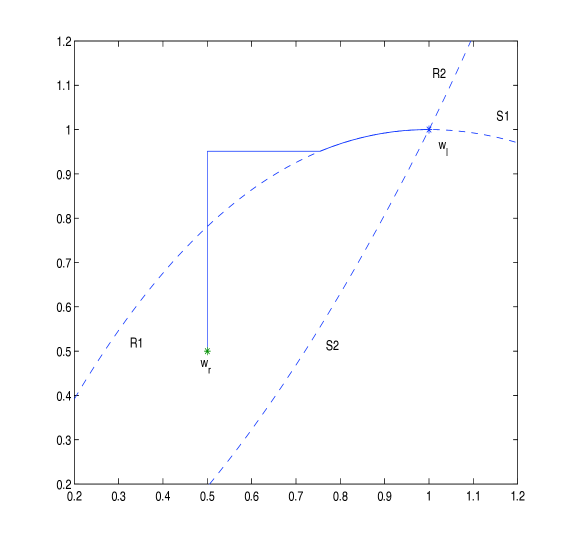
Once the jump conditions have been stated, it is possible to solve the Riemann problem for any pair of states which are sufficiently enough. Then, a family of paths satisfying (R2) and (R3) is constructed. In Figure 1 the path linking the states wl=[1,1]Tsubscript𝑤𝑙superscript11𝑇w_{l}=[1,1]^{T} and wr=[0.5,0.5]Tsubscript𝑤𝑟superscript0.50.5𝑇w_{r}=[0.5,0.5]^{T} is depicted. In this case, the solution of the Riemann problem consists of a 111-rarefaction connecting wlsubscript𝑤𝑙w_{l} to an intermediate state w~~𝑤\tilde{w} and a 222-shock linking w~~𝑤\tilde{w} to wrsubscript𝑤𝑟w_{r}. As a consequence, the path consists of the arc of the 1-integral curve linking wlsubscript𝑤𝑙w_{l} to w~~𝑤\tilde{w} and two segments connecting w~~𝑤\tilde{w} and wrsubscript𝑤𝑟w_{r} which are parallel to the axis . The set of states that can be connected to wlsubscript𝑤𝑙w_{l} by an entropy satisfying 1-wave or 2-wave are also depicted. In each case Ri𝑅𝑖Ri denotes i𝑖i-rarefactions and Si𝑆𝑖Si denotes i𝑖i-shocks.

Refer to caption
Figure 1: Path connecting the states wlsubscript𝑤𝑙w_{l} and wrsubscript𝑤𝑟w_{r} (continuous line) and set of states that can be connected to wlsubscript𝑤𝑙w_{l} by an entropy satisfying 1 or 2-wave (dashed lines).

4.2 A class of systems of balance laws

We consider PDE systems of the form:

wt+F(w)x=S(w)σx,subscript𝑤𝑡𝐹subscript𝑤𝑥𝑆𝑤subscript𝜎𝑥w_{t}+F(w)_{x}={S}(w)\sigma_{x}, (4.3)

where the unknown w(x,t)𝑤𝑥𝑡w(x,t) takes values on an open convex set 𝒪𝒪\mathcal{O} of Nsuperscript𝑁\mathbb{R}^{N}; F𝐹F and S𝑆S are regular functions from 𝒪𝒪\mathcal{O} to Nsuperscript𝑁\mathbb{R}^{N}; and σ(x)𝜎𝑥\sigma(x) is a known function from \mathbb{R} to \mathbb{R}. For an account of the existing literature on well-balanced schemes for this class of systems we refer to the lecture notes by Bouchut [4], as well as to the recent contribution by Noelle et al. [29], and Xin and Shu [33].

As pointed out in LeFloch [19] for the Euler equations in nozzle with discontinuous cross-section, such a system can be recast in the form of a nonconservative system Wt+A(W)Wx=0subscript𝑊𝑡𝐴𝑊subscript𝑊𝑥0W_{t}+A(W)W_{x}=0, by introducing

W=[wσ],A(W)=[J(w)S(w)00],formulae-sequence𝑊delimited-[]𝑤𝜎𝐴𝑊delimited-[]𝐽𝑤𝑆𝑤missing-subexpressionmissing-subexpression00W=\left[\begin{array}[]{c}w\\ \sigma\end{array}\right],\quad A(W)=\left[\begin{array}[]{c|c}J(w)&-{S}(w)\\ \hline\cr 0&0\end{array}\right],

where J(w)𝐽𝑤J(w) denotes the Jacobian matrix of F𝐹F:

J(w)=Fw(w).𝐽𝑤𝐹𝑤𝑤{J}(w)=\frac{\partial F}{\partial w}(w).

If J𝐽J has N𝑁N different real and non-vanishing eigenvalues λ1(w),,λN(w)subscript𝜆1𝑤subscript𝜆𝑁𝑤\lambda_{1}(w),\ldots,\lambda_{N}(w), then the system is strictly hyperbolic with eigenvalues

λ1(w),,λN(w),0.subscript𝜆1𝑤subscript𝜆𝑁𝑤0\lambda_{1}(w),\dots,\lambda_{N}(w),0.

Clearly, the (N+1)𝑁1(N+1)-th field is linearly degenerate and, for definiteness, we may assume that all other fields are genuinely nonlinear.

In order to define weak solutions to this nonconservative system, a family of paths

Φ(s;Wl,Wr)=[Φw(s;Wl,Wr)Φσ(s;Wl,Wr)]Φ𝑠subscript𝑊𝑙subscript𝑊𝑟delimited-[]subscriptΦ𝑤𝑠subscript𝑊𝑙subscript𝑊𝑟subscriptΦ𝜎𝑠subscript𝑊𝑙subscript𝑊𝑟\Phi(s;W_{l},W_{r})=\left[\begin{array}[]{c}\Phi_{w}(s;W_{l},W_{r})\\ \Phi_{\sigma}(s;W_{l},W_{r})\end{array}\right]

must be chosen and it is natural to impose the following requirement: if W=[w,σ]T𝑊superscript𝑤𝜎𝑇W=[w,\sigma]^{T} is a weak solution to the system and σ𝜎\sigma is a constant, then w𝑤w must be a weak solution of the system of conservation laws:

wt+F(w)x=0.subscript𝑤𝑡𝐹subscript𝑤𝑥0w_{t}+F(w)_{x}=0.

This requirement is satisfied if the family of paths fulfills the following condition:

  • (R4)

    If Wlsubscript𝑊𝑙{W}_{l} and Wrsubscript𝑊𝑟{W}_{r} are such that σl=σr=σ¯subscript𝜎𝑙subscript𝜎𝑟¯𝜎\sigma_{l}=\sigma_{r}=\bar{\sigma}, then:

    Φσ(s;Wl,Wr)=σ¯,s[0,1].formulae-sequencesubscriptΦ𝜎𝑠subscript𝑊𝑙subscript𝑊𝑟¯𝜎𝑠01{\Phi}_{\sigma}(s;{W}_{l},{W}_{r})=\bar{\sigma},\qquad s\in[0,1]. (4.4)

In fact any family of paths satisfying (R4) together with the requirements (R1) and (R3) (cf. Section 2.2), leads to the same notion of weak solution for such systems. These solutions contain two type of discontinuities :

  • Shock waves across which σ𝜎\sigma is continuous that satisfy the usual Rankine-Hugoniot conditions:

    ξ(w+w)=F(w+)F(w).𝜉superscript𝑤superscript𝑤𝐹superscript𝑤𝐹superscript𝑤\xi(w^{+}-w^{-})=F(w^{+})-F(w^{-}).
  • Stationary contact discontinuities placed at the jumps of σ𝜎\sigma and connecting two states that belong to the same integral curve of the linearly degenerate field.

For these systems, the difficulties of convergence commented above are not appreciated for the finite difference schemes introduced in Section 2.2. Moreover, the shock waves propagating in regions where σ𝜎\sigma is continuous are correctly captured independently of the choice of paths. Nevertheless, in order to correctly capture the stationary contact discontinuities related to the jumps of σ𝜎\sigma, the numerical schemes have to be based on families of paths that satisfy at least the requirement (R1). Interestingly, this is also the requirement necessary to obtain well-balanced schemes.

The Lax-Friedrichs scheme presented in Section 2.2 cannot be used as it stands for systems of balance laws as it does not preserve the equation

σt=0.subscript𝜎𝑡0\sigma_{t}=0.

In effect, it can be easily verified that the numerical scheme for the variable σ𝜎\sigma reads as follows:

σin+1=σi1n+σi+1n2.superscriptsubscript𝜎𝑖𝑛1superscriptsubscript𝜎𝑖1𝑛superscriptsubscript𝜎𝑖1𝑛2\sigma_{i}^{n+1}=\frac{\sigma_{i-1}^{n}+\sigma_{i+1}^{n}}{2}.

In [10] the following modification of the scheme was introduced to get rid of this difficulty: instead of (2.9), Mi+1/2n,±superscriptsubscript𝑀𝑖12𝑛plus-or-minusM_{i+1/2}^{n,\pm} are given by

Mi+1/2n,superscriptsubscript𝑀𝑖12𝑛\displaystyle M_{i+1/2}^{n,-} =A^i+1/2n,(ui+1nuin),absentsubscriptsuperscript^𝐴𝑛𝑖12superscriptsubscript𝑢𝑖1𝑛superscriptsubscript𝑢𝑖𝑛\displaystyle=\widehat{A}^{n,-}_{i+1/2}\cdot(u_{i+1}^{n}-u_{i}^{n}),
Mi+1/2n,+superscriptsubscript𝑀𝑖12𝑛\displaystyle M_{i+1/2}^{n,+} =A^i+1/2n,+(ui+1nuin),absentsubscriptsuperscript^𝐴𝑛𝑖12superscriptsubscript𝑢𝑖1𝑛superscriptsubscript𝑢𝑖𝑛\displaystyle=\widehat{A}^{n,+}_{i+1/2}\cdot(u_{i+1}^{n}-u_{i}^{n}),

where

A^i+1/2n,±=12(±ΔxΔtI^i+1/2n+Ai+1/2n).subscriptsuperscript^𝐴𝑛plus-or-minus𝑖1212plus-or-minusΔ𝑥Δ𝑡superscriptsubscript^𝐼𝑖12𝑛subscriptsuperscript𝐴𝑛𝑖12\widehat{A}^{n,\pm}_{i+1/2}=\frac{1}{2}\left(\pm\frac{\Delta x}{\Delta t}\widehat{I}_{i+1/2}^{n}+{A}^{n}_{i+1/2}\right).

Here, Ai+1/2nsubscriptsuperscript𝐴𝑛𝑖12{A}^{n}_{i+1/2} is a Roe linearization and

I^i+1/2n=𝒦i+1/2nId^(𝒦i+1/2n)1,superscriptsubscript^𝐼𝑖12𝑛superscriptsubscript𝒦𝑖12𝑛^𝐼𝑑superscriptsuperscriptsubscript𝒦𝑖12𝑛1\widehat{I}_{i+1/2}^{n}=\mathcal{K}_{i+1/2}^{n}\cdot\widehat{Id}\cdot(\mathcal{K}_{i+1/2}^{n})^{-1},

where 𝒦i+1/2nsuperscriptsubscript𝒦𝑖12𝑛\mathcal{K}_{i+1/2}^{n} is a matrix whose columns are eigenvectors of Ai+1/2nsuperscriptsubscript𝐴𝑖12𝑛A_{i+1/2}^{n} associated to λi+1/2,1nsuperscriptsubscript𝜆𝑖121𝑛\lambda_{i+1/2,1}^{n}, …, λi+1/2,Nnsuperscriptsubscript𝜆𝑖12𝑁𝑛\lambda_{i+1/2,N}^{n}, and Id^^𝐼𝑑\widehat{Id} is the diagonal matrix whose j𝑗j-th coefficient is 1 if λi+1/2,jn0superscriptsubscript𝜆𝑖12𝑗𝑛0\lambda_{i+1/2,j}^{n}\not=0, or 0 if λi+1/2,jn=0superscriptsubscript𝜆𝑖12𝑗𝑛0\lambda_{i+1/2,j}^{n}=0. Note that if, instead, I^i+1/2nsuperscriptsubscript^𝐼𝑖12𝑛\widehat{I}_{i+1/2}^{n} is taken to be equal to the identity matrix, then the Lax-Friedrichs scheme presented in Section 2.2 is recovered.

An important particular example of systems of balance laws is the shallow water system governing the flow of a shallow layer of inviscid homogeneous fluid through a straight channel with a constant rectangular cross-section:

ht+qx=0,𝑡𝑞𝑥0\displaystyle\frac{\partial h}{\partial t}+\frac{\partial q}{\partial x}=0, (4.5)
qt+x(q2h+g2h2)=ghdHdx.𝑞𝑡𝑥superscript𝑞2𝑔2superscript2𝑔d𝐻d𝑥\displaystyle\frac{\partial q}{\partial t}+\frac{\partial}{\partial x}\left({\frac{q^{2}}{h}+\frac{g}{2}h^{2}}\right)=gh\frac{\mbox{d}H}{\mbox{d}x}.

The variable x𝑥x makes reference to the axis of the channel and t𝑡t is time; q(x,t)𝑞𝑥𝑡q(x,t) and h(x,t)𝑥𝑡h(x,t) represent the mass-flow and the thickness, respectively; g𝑔g, the gravity; and H(x)𝐻𝑥H(x), the depth measured from a fixed level of reference.

The eigenvalues of this matrix are λ1=ucsubscript𝜆1𝑢𝑐\lambda_{1}=u-c, λ2=u+csubscript𝜆2𝑢𝑐\lambda_{2}=u+c, and 00, where c=gh𝑐𝑔c=\sqrt{gh}. In this case, the equations of the integral curves of the linearly degenerate field are given by the equations

q=const,h+q22gh2H=const.formulae-sequence𝑞𝑐𝑜𝑛𝑠𝑡superscript𝑞22𝑔superscript2𝐻𝑐𝑜𝑛𝑠𝑡q=const,\qquad h+\frac{q^{2}}{2gh^{2}}-H=const. (4.6)

The resonant regime where λ1subscript𝜆1\lambda_{1} or λ2subscript𝜆2\lambda_{2} vanish are not considered in the present paper; for a discussion of the Riemann problem see LeFloch and Thanh [27].

4.3 Two-layer shallow water system

We consider in this paragraph the system of partial differential equations governing the one-dimensional flow of two superposed immiscible layers of shallow water fluids over a flat bottom topography (see [8] for details) :

h1t+q1x=0,subscript1𝑡subscript𝑞1𝑥0\displaystyle{{\frac{\partial h_{1}}{\partial t}}+{\frac{\partial q_{1}}{\partial x}}=0,} (4.7)
q1t+x(q12h1+g2h12)=gh1h2x,subscript𝑞1𝑡𝑥superscriptsubscript𝑞12subscript1𝑔2superscriptsubscript12𝑔subscript1subscript2𝑥\displaystyle{\frac{\partial q_{1}}{\partial t}}+{\frac{\partial\ }{\partial x}}\left({\frac{q_{1}^{2}}{h_{1}}}+{\frac{g}{2}}h_{1}^{2}\right)=-gh_{1}{\frac{\partial h_{2}}{\partial x}},
h2t+q2x=0,subscript2𝑡subscript𝑞2𝑥0\displaystyle{{\frac{\partial h_{2}}{\partial t}}+{\frac{\partial q_{2}}{\partial x}}=0,}
q2t+x(q22h2+g2h22)=ρ1ρ2gh2h1x.subscript𝑞2𝑡𝑥superscriptsubscript𝑞22subscript2𝑔2superscriptsubscript22subscript𝜌1subscript𝜌2𝑔subscript2subscript1𝑥\displaystyle{{\frac{\partial q_{2}}{\partial t}}+{\frac{\partial\ }{\partial x}}\left({\frac{q_{2}^{2}}{h_{2}}}+{\frac{g}{2}}h_{2}^{2}\right)=-{\frac{\rho_{1}}{\rho_{2}}}gh_{2}{\frac{\partial h_{1}}{\partial x}}}.

In these equations, the index 1 refers to the upper layer and the index 2 to the lower one. The fluid is assumed to occupy a straight channel with constant rectangular cross-section and constant width. The coordinate x𝑥x refers to the axis of the channel, t𝑡t denotes the time variable, and g𝑔g is the gravity. Each layer is assumed to have a constant density ρisubscript𝜌𝑖\rho_{i}, i=1,2𝑖12i=1,2 (ρ1<ρ2subscript𝜌1subscript𝜌2\rho_{1}<\rho_{2}), while the unknowns qi(x,t)subscript𝑞𝑖𝑥𝑡q_{i}(x,t) and hi(x,t)subscript𝑖𝑥𝑡h_{i}(x,t) represent respectively the mass-flow and the thickness of the i𝑖i-th layer at the section of coordinate x𝑥x at time t𝑡t.

System (4.7) can be written in the form (1.1), say wt+A(w)wx=0subscript𝑤𝑡𝐴𝑤subscript𝑤𝑥0w_{t}+A(w)\,w_{x}=0, w=w(t,x)N𝑤𝑤𝑡𝑥superscript𝑁w=w(t,x)\in\mathbb{R}^{N}, with N=4𝑁4N=4 and

w=[h1q1h2q2],A(w)=[0100u12+c122u1c1200001rc220u22+c222u2],formulae-sequence𝑤delimited-[]subscript1subscript𝑞1subscript2subscript𝑞2𝐴𝑤delimited-[]0100superscriptsubscript𝑢12superscriptsubscript𝑐122subscript𝑢1superscriptsubscript𝑐1200001𝑟superscriptsubscript𝑐220superscriptsubscript𝑢22superscriptsubscript𝑐222subscript𝑢2w=\left[\begin{array}[]{c}h_{1}\\ q_{1}\\ h_{2}\\ q_{2}\\ \end{array}\right],\qquad A(w)=\left[\begin{array}[]{cccc}0&1&0&0\\ -u_{1}^{2}+c_{1}^{2}&2u_{1}&c_{1}^{2}&0\\ 0&0&0&1\\ rc_{2}^{2}&0&-u_{2}^{2}+c_{2}^{2}&2u_{2}\\ \end{array}\right],

where ui=qi/hisubscript𝑢𝑖subscript𝑞𝑖subscript𝑖u_{i}={q_{i}}/{h_{i}} represents the averaged velocity of the i𝑖i-th layer, ci=ghisubscript𝑐𝑖𝑔subscript𝑖c_{i}=\sqrt{gh_{i}}, i=1,2𝑖12i=1,2, and r=ρ1ρ2𝑟subscript𝜌1subscript𝜌2r=\frac{\rho_{1}}{\rho_{2}}. The characteristic equation of the system is

(λ22u1λ+u12gh1)(λ22u2λ+u22gh2)=rg2h1h2.superscript𝜆22subscript𝑢1𝜆superscriptsubscript𝑢12𝑔subscript1superscript𝜆22subscript𝑢2𝜆superscriptsubscript𝑢22𝑔subscript2𝑟superscript𝑔2subscript1subscript2\bigl{(}\lambda^{2}-2u_{1}\lambda+u_{1}^{2}-gh_{1}\bigr{)}\bigl{(}\lambda^{2}-2u_{2}\lambda+u_{2}^{2}-gh_{2}\bigr{)}=rg^{2}h_{1}h_{2}.

Observe that, when r=0𝑟0r=0, the eigenvalues are those corresponding to each layer separately. In this situation, the coupling terms do not affect the nature of the system in any essential manner.

In the case r1𝑟1r\cong 1 (which is the situation arising in many geophysical flows) a first-order approximation of the eigenvalues was given in [32]:

λext±superscriptsubscript𝜆extplus-or-minus\displaystyle\lambda_{\hbox{\scriptsize{ext}}}^{\pm} \displaystyle\cong u1h1+u2h2h1+h2±(g(h1+h2))1/2,plus-or-minussubscript𝑢1subscript1subscript𝑢2subscript2subscript1subscript2superscript𝑔subscript1subscript212\displaystyle{\frac{u_{1}h_{1}+u_{2}h_{2}}{h_{1}+h_{2}}}\pm\bigl{(}g(h_{1}+h_{2})\bigr{)}^{1/2}, (4.8)
λint±superscriptsubscript𝜆intplus-or-minus\displaystyle\lambda_{\hbox{\scriptsize{int}}}^{\pm} \displaystyle\cong u1h2+u2h1h1+h2±(gh1h2(h1+h2)(1(u1u2)2g(h1+h2)))1/2.plus-or-minussubscript𝑢1subscript2subscript𝑢2subscript1subscript1subscript2superscriptsuperscript𝑔subscript1subscript2subscript1subscript21superscriptsubscript𝑢1subscript𝑢22superscript𝑔subscript1subscript212\displaystyle{\frac{u_{1}h_{2}+u_{2}h_{1}}{h_{1}+h_{2}}}\pm\left(g^{\prime}{\frac{h_{1}h_{2}}{(h_{1}+h_{2})}}\Bigl{(}1-{\frac{(u_{1}-u_{2})^{2}}{g^{\prime}(h_{1}+h_{2})}}\Bigr{)}\right)^{1/2}. (4.9)

In the former expression, g=(1r)gsuperscript𝑔1𝑟𝑔g^{\prime}=(1-r)g is the reduced gravity.

It is not easy to check the genuinely nonlinear character of the 4 characteristic fields, as the eigenvalues and eigenvectors can not be written explicitely in a simple manner. Nevertheless, this fact is easily proved in the case r=0𝑟0r=0 as, in this case, the system reduces to two decoupled shallow water systems. As a consequence, using a continuity argument, this is also true at least for small values of r𝑟r.

From equation (4.9) we can observe that the internal eigenvalues may become complex. This situation occurs when they satisfy, approximately, the following inequality:

(u1u2)2g(h1+h2)>1.superscriptsubscript𝑢1subscript𝑢22superscript𝑔subscript1subscript21{\frac{(u_{1}-u_{2})^{2}}{g^{\prime}(h_{1}+h_{2})}}>1.

In this case, the system loses its hyperbolic character. These situations are related with the appearance of shear instabilities that may lead, in real flows, to intense mixing of the two layers. While, in practice, this mixture partially dissipates the energy, in numerical experiments these interface disturbances grow and overwhelm the solution. Clearly, we cannot expect to simulate these phenomena with a two-immiscible-layer model. Therefore, the above inequality in fact gives the range of validity of a model based on the equations (4.7), if viscosity effects are neglected. In this work only the case where the matrix A(w)𝐴𝑤{A}({w}) has real eigenvalues is considered, i.e. the system is supposed to be strictly hyperbolic.

The jump conditions (3.3) related to the choice of a family of paths

Φ(s;wl,wr)=[Φh1(s;wl,wr)Φq1(s;wl,wr)Φh2(s;wl,wr)Φq2(s;wl,wr)]Φ𝑠subscript𝑤𝑙subscript𝑤𝑟delimited-[]subscriptΦsubscript1𝑠subscript𝑤𝑙subscript𝑤𝑟subscriptΦsubscript𝑞1𝑠subscript𝑤𝑙subscript𝑤𝑟subscriptΦsubscript2𝑠subscript𝑤𝑙subscript𝑤𝑟subscriptΦsubscript𝑞2𝑠subscript𝑤𝑙subscript𝑤𝑟\Phi(s;w_{l},w_{r})=\left[\begin{array}[]{c}\Phi_{h_{1}}(s;w_{l},w_{r})\\ \Phi_{q_{1}}(s;w_{l},w_{r})\\ \Phi_{h_{2}}(s;w_{l},w_{r})\\ \Phi_{q_{2}}(s;w_{l},w_{r})\end{array}\right]

read

ξ(h1rh1l)=𝜉superscriptsubscript1𝑟superscriptsubscript1𝑙absent\displaystyle\xi{(h_{1}^{r}-h_{1}^{l})}= q1rq1l,superscriptsubscript𝑞1𝑟superscriptsubscript𝑞1𝑙\displaystyle{q_{1}^{r}-q_{1}^{l}}, (4.10)
ξ(q1rq1l)=𝜉superscriptsubscript𝑞1𝑟superscriptsubscript𝑞1𝑙absent\displaystyle\xi{(q_{1}^{r}-q_{1}^{l})}= (q1r)2h1r(q1l)2h1l+g2(h1r)2g2(h1l)2superscriptsuperscriptsubscript𝑞1𝑟2superscriptsubscript1𝑟superscriptsuperscriptsubscript𝑞1𝑙2superscriptsubscript1𝑙𝑔2superscriptsuperscriptsubscript1𝑟2𝑔2superscriptsuperscriptsubscript1𝑙2\displaystyle{\frac{(q_{1}^{r})^{2}}{h_{1}^{r}}-\frac{(q_{1}^{l})^{2}}{h_{1}^{l}}+\frac{g}{2}(h_{1}^{r})^{2}-\frac{g}{2}(h_{1}^{l})^{2}}
+g01Φh1(s;wl,wr)Φh2s(s;wl,wr)𝑑s,𝑔superscriptsubscript01subscriptΦsubscript1𝑠subscript𝑤𝑙subscript𝑤𝑟subscriptΦsubscript2𝑠𝑠subscript𝑤𝑙subscript𝑤𝑟differential-d𝑠\displaystyle{+g\int_{0}^{1}\Phi_{h_{1}}(s;w_{l},w_{r})\frac{\partial\Phi_{h_{2}}}{\partial s}(s;w_{l},w_{r})\,ds},
ξ(h2rh2l)=𝜉superscriptsubscript2𝑟superscriptsubscript2𝑙absent\displaystyle\xi{(h_{2}^{r}-h_{2}^{l})}= q2rq2l,superscriptsubscript𝑞2𝑟superscriptsubscript𝑞2𝑙\displaystyle{q_{2}^{r}-q_{2}^{l}},
ξ(q2rq2l)=𝜉superscriptsubscript𝑞2𝑟superscriptsubscript𝑞2𝑙absent\displaystyle\xi{(q_{2}^{r}-q_{2}^{l})}= (q2r)2h2r(q2l)2h2l+g2(h2r)2g2(h2l)2superscriptsuperscriptsubscript𝑞2𝑟2superscriptsubscript2𝑟superscriptsuperscriptsubscript𝑞2𝑙2superscriptsubscript2𝑙𝑔2superscriptsuperscriptsubscript2𝑟2𝑔2superscriptsuperscriptsubscript2𝑙2\displaystyle{\frac{(q_{2}^{r})^{2}}{h_{2}^{r}}-\frac{(q_{2}^{l})^{2}}{h_{2}^{l}}+\frac{g}{2}(h_{2}^{r})^{2}-\frac{g}{2}(h_{2}^{l})^{2}}
+gr01Φh2(s;wl,wr)Φh1s(s;wl,wr)𝑑s.𝑔𝑟superscriptsubscript01subscriptΦsubscript2𝑠subscript𝑤𝑙subscript𝑤𝑟subscriptΦsubscript1𝑠𝑠subscript𝑤𝑙subscript𝑤𝑟differential-d𝑠\displaystyle{+gr\int_{0}^{1}\Phi_{h_{2}}(s;w_{l},w_{r})\frac{\partial\Phi_{h_{1}}}{\partial s}(s;w_{l},w_{r})\,ds.}

Observe that these conditions are independent of the choice of Φqi(s:wl,wr)\Phi_{q_{i}}(s:w_{l},w_{r}), i=1,2𝑖12i=1,2.

Refer to caption
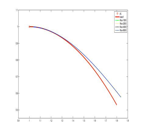
Figure 2: Test case 5.1. Hugoniot curves: exact (continuous red line) and numerical (line with dots) obtained with Roe scheme

5 Numerical experiments

5.1 A simplified system

We will demonstrate here that, in general, a difference scheme for a general nonconservative hyperbolic system (1.1) does not converge to the exact solution u𝑢u, that is, with the notation already introduced in previous sections we claim that

v=limΔ0uΔu.𝑣subscriptΔ0superscript𝑢Δ𝑢v=\lim_{\Delta\to 0}u^{\Delta}\neq u. (5.1)

This fact was first observed for nonconservative schemes for scalar equations in Hou and LeFloch [16] and, in the context of nonclassical shocks generated by diffusion and dispersion, in Hayes and LeFloch [15, 25]. Here, we observe (5.1) for finite difference approximations of nonconservative systems.
Refer to caption
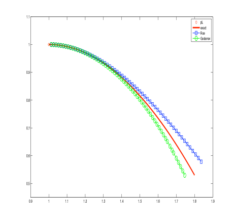
Figure 3: Test case 5.1. Hugoniot curves: exact (continuous red line), Roe (blue line with squares) and Godunov (green line with circles)

We begin with the convergence of Roe and Godunov methods for (4.1). The Roe method considered here is consistent with the family of paths given by (4.2) for every pair of states. The corresponding Roe matrix is as follows:

Ai+1/2n=[01(ui+1/2n)2+qinhi+1/2n2ui+1/2n],superscriptsubscript𝐴𝑖12𝑛delimited-[]01superscriptsuperscriptsubscript𝑢𝑖12𝑛2superscriptsubscript𝑞𝑖𝑛superscriptsubscript𝑖12𝑛2subscriptsuperscript𝑢𝑛𝑖12A_{i+1/2}^{n}=\left[\begin{array}[]{cc}0&1\\ -(u_{i+1/2}^{n})^{2}+q_{i}^{n}h_{i+1/2}^{n}&2u^{n}_{i+1/2}\end{array}\right],

where

ui+1/2n=hinuin+hi+1nui+1nhin+hi+1n,hi+1/2n=12(hin+hi+1n).formulae-sequencesuperscriptsubscript𝑢𝑖12𝑛superscriptsubscript𝑖𝑛superscriptsubscript𝑢𝑖𝑛superscriptsubscript𝑖1𝑛superscriptsubscript𝑢𝑖1𝑛superscriptsubscript𝑖𝑛superscriptsubscript𝑖1𝑛superscriptsubscript𝑖12𝑛12superscriptsubscript𝑖𝑛superscriptsubscript𝑖1𝑛u_{i+1/2}^{n}=\frac{\sqrt{h_{i}^{n}}u_{i}^{n}+\sqrt{h_{i+1}^{n}}u_{i+1}^{n}}{\sqrt{h_{i}^{n}}+\sqrt{h_{i+1}^{n}}},\quad h_{i+1/2}^{n}=\frac{1}{2}(h_{i}^{n}+h_{i+1}^{n}).

On the other hand, the Godunov method considered here is based on the family of paths described in Section 4.1: it satisfies (R2)-(R3) and coincides with (4.2) for pair of states that can be linked by a shock.

We consider the Rankine-Hugoniot curve composed by the states wrsubscript𝑤𝑟w_{r} that can connected with wl=[1;1]Tsubscript𝑤𝑙superscript11𝑇w_{l}=[1;1]^{T} by a 1-shock, which is given by:

qr=hr(1hr+12hr(hr1)).subscript𝑞𝑟subscript𝑟1subscript𝑟12subscript𝑟subscript𝑟1q_{r}=h_{r}\left(1-\sqrt{\frac{h_{r}+1}{2h_{r}}}(h_{r}-1)\right). (5.2)

Figure 2 shows a plot of the curve (5.2) in the plane hq𝑞h-q (continuous red line).

Refer to caption
(a) h at t=0.5𝑡0.5t=0.5
Refer to caption
(b) h (zoom) at t=0.5𝑡0.5t=0.5.
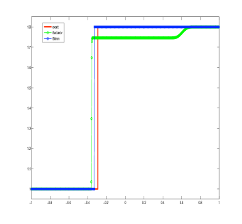
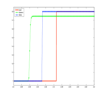
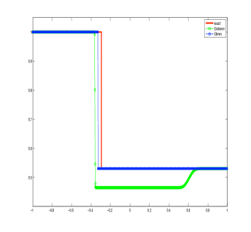
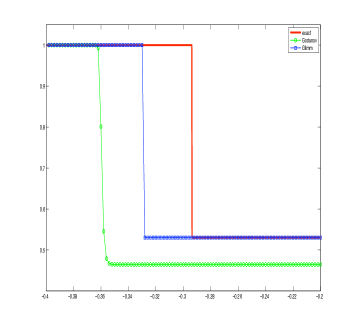
Figure 4: Test case 5.1. Solution of Riemann problem (hh) (5.3) at time t=0.5𝑡0.5t=0.5: Exact (continuous red line), Godunov (green line with circles) and Glimm (blue line with squares)
Refer to caption
(a) q at t=0.5𝑡0.5t=0.5
Refer to caption
(b) q (zoom) at t=0.5𝑡0.5t=0.5.
Figure 5: Test case 5.1. Solution of Riemann problem (q𝑞q) (5.3) at time t=0.5𝑡0.5t=0.5: Exact (continuous red line), Godunov (green line with circles) and Glimm (blue line with squares)

Next, Roe method is used to solve numerically a family of Riemann problems in which the left state is wlsubscript𝑤𝑙w_{l} and the right state wrsubscript𝑤𝑟w_{r} runs on the Hugoniot curve (5.2). The speed of propagation and the limit states of the 1-shock are computed in the numerical solution by using the first divided difference as a smooth indicator. This computation has been performed using four meshes with decreasing mesh step (Δx=0.002Δ𝑥0.002\Delta x=0.002, Δx=0.001Δ𝑥0.001\Delta x=0.001, Δx=0.0005Δ𝑥0.0005\Delta x=0.0005 and Δx=0.00025Δ𝑥0.00025\Delta x=0.00025). The CFL parameter is set to 0.90.90.9. The numerical Hugoniot curves obtained in this way (line with dots) are compared with the exact one (continuous red line) in Figure 2. It can be observed that the numerical Hugoniot curves converge, but the limit is not the exact one.

The same behavior is observed for Godunov method: the numerical Hugoniot-curves converge but the limit is not the exact one: in Figure 3 the exact Hugoniot curve (continuous red line) is compared with those computed with Roe (blue line with squares) and Godunov (green line with circles) methods with Δx=0.001Δ𝑥0.001\Delta x=0.001. The CLF parameter is set to 0.90.90.9 for Roe and 0.50.50.5 for Godunov. This choice ensures that the Godunov method corresponds to advance in time by exactly solving the Riemann problems and taking the averages of the solutions at the cells.

Finally, we compare Godunov and Glimm methods. We consider a Riemann problem with initial conditions

w(x,0)={wl=(11),x<0;wr=(1.8qr),x>0;𝑤𝑥0casessubscript𝑤𝑙11𝑥0missing-subexpressionmissing-subexpressionsubscript𝑤𝑟1.8subscript𝑞𝑟𝑥0w(x,0)=\left\{\begin{array}[]{lr}w_{l}=\left(\begin{array}[]{c}1\\ 1\end{array}\right),&x<0;\\ \\ w_{r}=\left(\begin{array}[]{c}1.8\\ q_{r}\end{array}\right),&x>0;\end{array}\right. (5.3)

where qrsubscript𝑞𝑟q_{r} is given by (5.2) for hr=1.8subscript𝑟1.8h_{r}=1.8 (qr0.530039370688997subscript𝑞𝑟0.530039370688997q_{r}\cong 0.530039370688997). The exact solution consists thus of a 1-shock linking the states. In Figures 4 and 5 the exact solution at time t=0.5𝑡0.5t=0.5 is compared with numerical solutions obtained with Godunov (green line with circles) and Glimm (blue line with squares) methods with Δx=0.001Δ𝑥0.001\Delta x=0.001 and CFL=0.50.50.5. Note how Godunov method introduces a 2-rarefaction in the computed solution.

Observe that the first equation of (4.1) is a conservation law. According to this equation, for A>0𝐴0A>0 large enough, the exact solution of the Riemann problem has to satisfy the following conservation property:

AAh(x,t)𝑑x=AAh(x,0)𝑑x+t(1qr).superscriptsubscript𝐴𝐴𝑥𝑡differential-d𝑥superscriptsubscript𝐴𝐴𝑥0differential-d𝑥𝑡1subscript𝑞𝑟\int_{-A}^{A}h(x,t)\,dx=\int_{-A}^{A}h(x,0)\,dx+t(1-q_{r}).

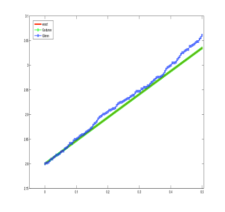
In Figure 6 we investigate the conservation property of both Godunov and Glimm methods: we fix A𝐴A and compare the exact value of the integral of hh at time tnsubscript𝑡𝑛t_{n} with its numerical approximations. Note that Godunov method satisfies the conservation property exactly.
Refer to caption
Figure 6: Test case 5.1. Evolution of the ‘mass’: exact (continuous red line), Glimm (blue line with squares) and Godunov (green line with circles)

5.2 Shallow water system

In this section we consider the discretization of the shallow water system by means of Roe and the modified Lax-Friedrichs schemes applied to the formulation (1.1) of the problem. In the first test, we check that, for continuous bottom functions H𝐻H, the shock waves are correctly captured for the schemes even if the numerical schemes are formally consistent with a simple family of paths. In the second one, stationary contact discontinuities placed at the jumps of H𝐻H are considered: we check that they are correctly captured only when the family of paths satisfies the property (R1).

5.2.1 Dam-break problem over a non-flat bottom topography

The axis of the channel is the interval [0,10]010[0,10] and the bottom topography is given by the function H(x)=10.5e(x5)2𝐻𝑥10.5superscript𝑒superscript𝑥52\displaystyle H(x)=1-0.5e^{-(x-5)^{2}}. The initial condition is q=0𝑞0q=0 and

h(x)={H(x),x4;H(x)+0.5,x<4.𝑥cases𝐻𝑥𝑥4missing-subexpressionmissing-subexpression𝐻𝑥0.5𝑥4h(x)=\left\{\begin{array}[]{ll}\displaystyle H(x),&\qquad\text{$x\geq 4$};\\ \\ H(x)+0.5,&\qquad\text{$x<4$}.\end{array}\right.

The final time is t=0.6𝑡0.6t=0.6. Free boundary conditions are considered. The CFL parameter is set to 0.90.90.9.

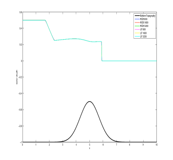
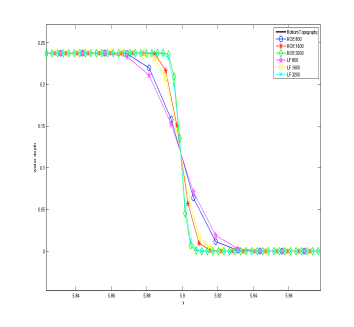
We consider a Roe scheme and a modified Lax-Friedrichs scheme which are consistent with the family of segments. Figure 7 shows the bottom topography and the free surface computed for both schemes using three meshes with increasing number of cells (800, 1600 and 3200 cells respectively). Both schemes converge to the same solution. Moreover, the speed of propagation ξ𝜉\xi and the limit states wsuperscript𝑤w^{-} and w+superscript𝑤w^{+} of the shock in the numerical solutions have been computed for both schemes by using a fine mesh of 32000 cells and the first divided difference as a smooth indicator. The value of the residual |ξ(w+w)F(w+)+F(w)|𝜉superscript𝑤superscript𝑤𝐹superscript𝑤𝐹superscript𝑤|\xi(w^{+}-w^{-})-F(w^{+})+F(w^{-})| obtained for the well-balanced Lax-Friedrichs scheme is 0.0080.0080.008 and for Roe scheme, 0.0060.0060.006.

Refer to caption
(a) Bottom topography and free surface at t=0.6.
Refer to caption
(b) Free surface (zoom) at t=0.6.
Figure 7: Test case 5.2.1. Dam-break problem: bottom topography and free surface at t=0.6.

5.2.2 Stationary contact discontinuities

In this test we study the approximation of stationary contact discontinuities. Following the discussion in Section 4.2, such a discontinuity has to connect two states belonging to a same curve of the family (4.6). As the family of segments only satisfies (R1) for the particular case of the curves

q=0,hH=const,formulae-sequence𝑞0𝐻𝑐𝑜𝑛𝑠𝑡q=0,\ h-H=const,

the Roe and the modified Lax-Friedrichs schemes based on the family of segments are only expected to capture correctly stationary contact discontinuities corresponding to water at rest over a discontinuous bottom. To check this in practice, we consider a channel whose axis is the interval [5,5]55[-5,5] and whose bottom is given by the function

H(x)={0,x<0,1,x>=0.𝐻𝑥cases0missing-subexpression𝑥01missing-subexpression𝑥0H(x)=\left\{\begin{array}[]{cll}0,&&x<0,\\ 1,&&x>=0.\end{array}\right.

We consider the initial condition:

wl=[hlq]=[14g],wr=[hr4g],formulae-sequencesubscript𝑤𝑙delimited-[]subscript𝑙𝑞delimited-[]14𝑔subscript𝑤𝑟delimited-[]subscript𝑟4𝑔w_{l}=\left[\begin{array}[]{c}h_{l}\\ q\end{array}\right]=\left[\begin{array}[]{c}1\\ \sqrt{4g}\end{array}\right],\qquad\quad w_{r}=\left[\begin{array}[]{c}h_{r}\\ \sqrt{4g}\end{array}\right],

where hrsubscript𝑟h_{r} has been calculated so that both states belong to the same integral curve (4.6) (hr0.7892441190408083subscript𝑟0.7892441190408083h_{r}\cong 0.7892441190408083). The exact solution of this Riemann problem is thus a stationary contact discontinuity.

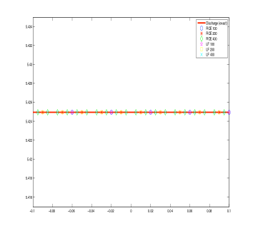
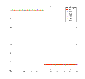
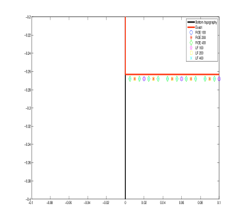
We have applied both schemes to this Riemann problem. As boundary condition, the state wlsubscript𝑤𝑙w_{l} is imposed upstream and free boundary conditions downstream. The CLF parameter is set to 0.9. Figures 8 and 9 show the stationary solutions obtained with both schemes using three meshes with increasing number of cells (100, 200 and 400 cells respectively). As expected, the numerical solutions do not converge to the exact solution. Note that both schemes converge to the same discontinuous function.
Refer to caption
(a) Bottom topography and free surface (stationary solution).
Refer to caption
(b) Bottom topography and free surface (stationary solution): zoom
Figure 8: Test case 5.2.2. Stationary contact discontinuity: Comparison between the modified Lax-Friedrichs and Roe schemes and the exact solution (free surface).
Refer to caption
Figure 9: Test case 5.2.2. Stationary contact discontinuity: Comparison between the well-balanced Lax-Friedrichs and Roe schemes and the exact solution (discharge).

Let us check what happens if the numerical schemes are based on a family of paths satisfying (R1) for every integral curve of the linearly degenerate field. We consider the family of paths constructed in [9] in order to design a Roe scheme which is well-balanced for every smooth stationary solution. The path connecting two states Wlsubscript𝑊𝑙W_{l} and Wrsubscript𝑊𝑟W_{r} consists of an arc of one of the curves of the family (4.6) and a segment lying on a plane H=const𝐻𝑐𝑜𝑛𝑠𝑡H=const: see [9] for details. Once the corresponding Roe matrix has been calculated, the construction of the modified Lax-Friedrichs scheme is straightforward.

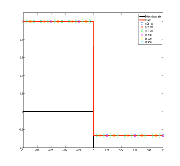
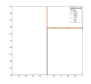
Figure 10 shows the comparison between Roe, the modified Lax-Friedrichs scheme, and the exact solution for three meshes with increasing number of cells (100, 200 and 400 cells respectively). As expected, the stationary contact discontinuity is exactly captured.
Refer to caption
(a) Bottom topography and free surface (stationary solution).
Refer to caption
(b) Bottom topography and free surface (stationary solution): zoom
Figure 10: Test case 5.2.2. Stationary contact discontinuity: Comparison between the exactly well-balanced Lax-Friedrichs and Roe schemes and the exact solution (free surface).

5.3 Two-layer shallow water system

5.3.1 Approximation of internal shocks

In this section we consider the discretization of the homogeneous two-layer shallow water system (that is, H=cst.𝐻𝑐𝑠𝑡H=cst.) by means of Roe and Lax-Friedrichs schemes. We check that the numerical solutions do not converge to the weak solutions involving shocks even when the same family of paths is used both for the definition of the jump conditions and the construction of the numerical scheme.

We begin with the family of segments for the definition of the jump condition (4.10). In this case:

01Φh1(s;wl,wr)Φh2s(s;wl,wr)𝑑s=h1l+h1r2(h2rh2l),superscriptsubscript01subscriptΦsubscript1𝑠subscript𝑤𝑙subscript𝑤𝑟subscriptΦsubscript2𝑠𝑠subscript𝑤𝑙subscript𝑤𝑟differential-d𝑠superscriptsubscript1𝑙superscriptsubscript1𝑟2superscriptsubscript2𝑟superscriptsubscript2𝑙\displaystyle\int_{0}^{1}\Phi_{h_{1}}(s;w_{l},w_{r})\frac{\partial\Phi_{h_{2}}}{\partial s}(s;w_{l},w_{r})\,ds=\frac{h_{1}^{l}+h_{1}^{r}}{2}(h_{2}^{r}-h_{2}^{l}),
01Φh2(s;wl,wr)Φh1s(s;wl,wr)𝑑s=h2l+h2r2(h1rh1l).superscriptsubscript01subscriptΦsubscript2𝑠subscript𝑤𝑙subscript𝑤𝑟subscriptΦsubscript1𝑠𝑠subscript𝑤𝑙subscript𝑤𝑟differential-d𝑠superscriptsubscript2𝑙superscriptsubscript2𝑟2superscriptsubscript1𝑟superscriptsubscript1𝑙\displaystyle\int_{0}^{1}\Phi_{h_{2}}(s;w_{l},w_{r})\frac{\partial\Phi_{h_{1}}}{\partial s}(s;w_{l},w_{r})\,ds=\frac{h_{2}^{l}+h_{2}^{r}}{2}(h_{1}^{r}-h_{1}^{l}).

In all of the cases considered here the order of the eigenvalues of the system is:

λext<λint<λint+<λext+.superscriptsubscript𝜆𝑒𝑥𝑡superscriptsubscript𝜆𝑖𝑛𝑡superscriptsubscript𝜆𝑖𝑛𝑡superscriptsubscript𝜆𝑒𝑥𝑡\lambda_{ext}^{-}<\lambda_{int}^{-}<\lambda_{int}^{+}<\lambda_{ext}^{+}.

Moreover

|λint±|<<|λext±|.much-less-thansuperscriptsubscript𝜆𝑖𝑛𝑡plus-or-minussuperscriptsubscript𝜆𝑒𝑥𝑡plus-or-minus|\lambda_{int}^{\pm}|<<|\lambda_{ext}^{\pm}|. (5.4)

We consider first a Lax-Friedrichs scheme consistent with the family of segments. Some easy calculations show that, for the particular choice of the family of segments, the last term in the modified equation (3.1) vanishes.

The goal is to compare the exact and the numerical Hugoniot curves corresponding to one of the internal characteristic fields; i.e. the fields related to the eigenvalues λint±superscriptsubscript𝜆𝑖𝑛𝑡plus-or-minus\lambda_{int}^{\pm}). We proceed as follows: the state

wr=[h1rq1rh2rq2r]=[0.3920341610254720.1988269593961961.5888290110974820.186046955388750]subscript𝑤𝑟delimited-[]superscriptsubscript1𝑟superscriptsubscript𝑞1𝑟superscriptsubscript2𝑟superscriptsubscript𝑞2𝑟delimited-[]0.3920341610254720.1988269593961961.5888290110974820.186046955388750w_{r}=\left[\begin{array}[]{c}h_{1}^{r}\\ q_{1}^{r}\\ h_{2}^{r}\\ q_{2}^{r}\end{array}\right]=\left[\begin{array}[]{c}0.392034161025472\\ -0.198826959396196\\ 1.588829011097482\\ 0.186046955388750\end{array}\right] (5.5)

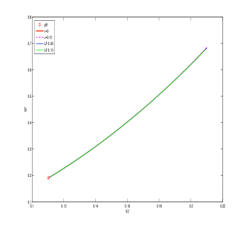
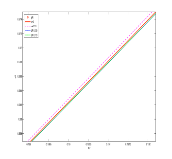
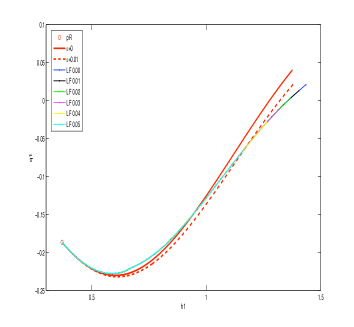
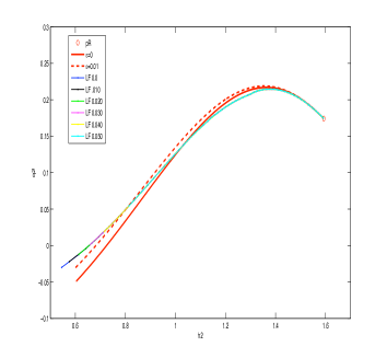
is fixed. Then, we compute the Hugoniot curve corresponding to the ‘left ’states wlsubscript𝑤𝑙w_{l} that can be connected with wrsubscript𝑤𝑟w_{r} with a 3-shock. To do this, we use the speed of the shock ξ𝜉\xi as a parameter and, for each value of ξ𝜉\xi we solve the non-linear system (4.10). In Figure 11 we show the projection (continuous blue line) of the computed Hugoniot curve onto the planes h1q1subscript1subscript𝑞1h_{1}-q_{1} (left) and h2q2subscript2subscript𝑞2h_{2}-q_{2} (right), respectively.

Next, we solve numerically a family of Riemann problems in which the right state is wrsubscript𝑤𝑟w_{r}, while wlsubscript𝑤𝑙w_{l} runs on the Hugoniot curve. Using the first divided difference as a smooth indicator, the speed of propagation and the limit states of the shock corresponding to the eigenvalue λint+superscriptsubscript𝜆𝑖𝑛𝑡\lambda_{int}^{+} is determined in the numerical solution. These calculations have been performed by using four meshes with decreasing step ( Δx=0.002Δ𝑥0.002\Delta x=0.002, 0.0010.0010.001, 0.00050.00050.0005 and 0.000250.000250.00025). The numerical Hugoniot curves so obtained are compared with the exact one in Figure 11. Observe that the numerical solutions converge, but the limit is not a weak solution according to the chosen family of paths. Nevertheless, if wrsubscript𝑤𝑟w_{r} and wlsubscript𝑤𝑙w_{l} are close enough, both curves are very close. The same behaviour can be observed if the shock speed is close to zero: this situation corresponds in the figure to the intersections of the curves.
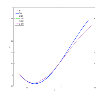
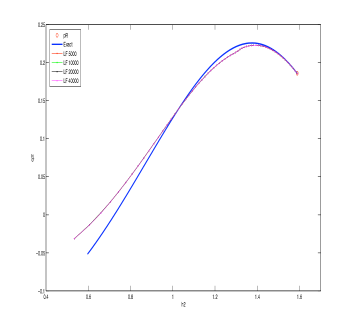
Refer to caption
(a) Hugoniot curves (projection onto the plane h1q1subscript1subscript𝑞1h_{1}-q_{1}): exact (continuous blue line) and numerical (lines with dots)
Refer to caption
(b) Hugoniot curves (projection onto the plane h2q2subscript2subscript𝑞2h_{2}-q_{2}): exact (continuous blue line) and numerical (lines with dots)
Figure 11: Test case 5.3.1. Hugoniot curves: exact (continuous blue line) and numerical (lines with dots).

A similar behavior is observed for Roe scheme: the numerical approximations converge but the limit is not a weak solution according to the family of segments. Nevertheless, as the numerical viscosity of the scheme is smaller than that corresponding to Lax-Friedrichs, the results are expected to be closer to the exact solution: in Figure 12 we compare the exact Hugoniot curve with those computed with Lax-Friedrichs and Roe schemes using a mesh with 10000 cells.
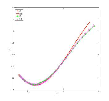
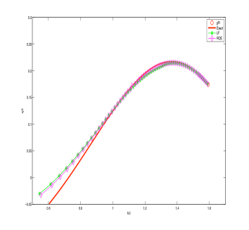
Refer to caption
(a) Hugoniot curves (projection onto the plane h1q1subscript1subscript𝑞1h_{1}-q_{1}): exact (continuous red line) and numerical (lines with dots)
Refer to caption
(b) Hugoniot curves (projection onto the plane h2q2subscript2subscript𝑞2h_{2}-q_{2}): exact (continuous red line) and numerical (lines with dots)
Figure 12: Test case 5.3.1. Hugoniot curves: exact (continuous red line) and numerical (lines with dots).

5.3.2 Approximation of external shocks

Due to the inequality (5.4) the CFL condition adjusts the numerical velocity to the external eigenvalues. As a consequence the effects of the numerical viscosity are much stronger for internal shocks and thus external shocks are expected to be better captured with Lax-Friedrichs or Roe schemes.

In order to check this, we proceed as in the previous test case: the state wrsubscript𝑤𝑟w_{r} given by

wr=[0.2573814695915670.4449016541886810.1103063440934180.190672137450279]subscript𝑤𝑟delimited-[]0.2573814695915670.4449016541886810.1103063440934180.190672137450279w_{r}=\left[\begin{array}[]{c}0.257381469591567\\ 0.444901654188681\\ 0.110306344093418\\ 0.190672137450279\end{array}\right]

is fixed, and then the Hugoniot curves corresponding to the ‘left ’states (wlsubscript𝑤𝑙w_{l}) that can be connected with wrsubscript𝑤𝑟w_{r} with a shock related to the eigenvalue λextsubscriptsuperscript𝜆𝑒𝑥𝑡\lambda^{-}_{ext} are computed by solving the non-linear system (4.10) using ξ𝜉\xi as a parameter.

In Figure 13 we compare the exact Hugoniot curve with those computed with Lax-Friedrichs and Roe scheme using a mesh with 2000 cells. Note how the curves are now much closer to each other than they were in the previous test case.
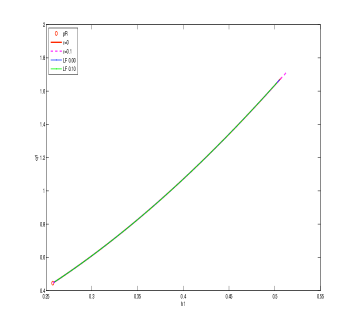
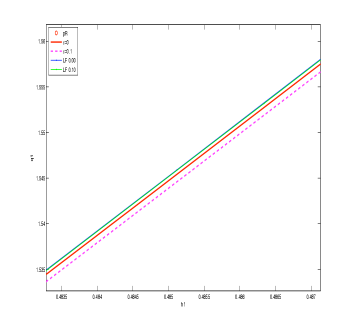
Refer to caption
(a) Hugoniot curves (projection onto the plane h1q1subscript1subscript𝑞1h_{1}-q_{1}): exact (continuous red line) and numerical (lines with dots)
Refer to caption
(b) Hugoniot curves (zoom of the projection onto the plane h1q1subscript1subscript𝑞1h_{1}-q_{1}): exact (continuous red line) and numerical (lines with dots)
Refer to caption
(c) Hugoniot curves (projection onto the plane h2q2subscript2subscript𝑞2h_{2}-q_{2}): exact (continuous red line) and numerical (lines with dots)
Refer to caption
(d) Hugoniot curves (zoom of the projection onto the plane h2q2subscript2subscript𝑞2h_{2}-q_{2}): exact (continuous red line) and numerical (lines with dots)
Figure 13: Test case 5.3.2. Hugoniot curves for Lax-Friedrichs and Roe schemes: exact (continuous red line) and numerical (lines with dots).

5.4 Influence of the family of paths

In this test we study the influence of small changes in the family of paths both in the weak and the numerical solutions. We consider now the jump conditions related to a different family of paths Φhiϵ(s;wl,wr)subscriptsuperscriptΦitalic-ϵsubscript𝑖𝑠subscript𝑤𝑙subscript𝑤𝑟\Phi^{\epsilon}_{h_{i}}(s;w_{l},w_{r}), i=1,2𝑖12i=1,2. These curves are chosen so that:

h1=Φh1ϵ(s;wl,wr),s[0,1];formulae-sequencesubscript1subscriptsuperscriptΦitalic-ϵsubscript1𝑠subscript𝑤𝑙subscript𝑤𝑟𝑠01\displaystyle h_{1}=\Phi^{\epsilon}_{h_{1}}(s;w_{l},w_{r}),\quad s\in[0,1];
h2=Φh2ϵ(s;wl,wr),s[0,1];formulae-sequencesubscript2subscriptsuperscriptΦitalic-ϵsubscript2𝑠subscript𝑤𝑙subscript𝑤𝑟𝑠01\displaystyle h_{2}=\Phi^{\epsilon}_{h_{2}}(s;w_{l},w_{r}),\quad s\in[0,1];

is a parameterization of the curve

h2=h2l+(h1h1lh1rh1l+ϵ(h1r)2(h1l)2(h1r)2(h1l)2)h2rh2l1+ϵ.subscript2superscriptsubscript2𝑙subscript1superscriptsubscript1𝑙superscriptsubscript1𝑟superscriptsubscript1𝑙italic-ϵsuperscriptsuperscriptsubscript1𝑟2superscriptsuperscriptsubscript1𝑙2superscriptsuperscriptsubscript1𝑟2superscriptsuperscriptsubscript1𝑙2superscriptsubscript2𝑟superscriptsubscript2𝑙1italic-ϵh_{2}=h_{2}^{l}+\left(\frac{h_{1}-h_{1}^{l}}{h_{1}^{r}-h_{1}^{l}}+\epsilon\frac{(h_{1}^{r})^{2}-(h_{1}^{l})^{2}}{(h_{1}^{r})^{2}-(h_{1}^{l})^{2}}\right)\frac{h_{2}^{r}-h_{2}^{l}}{1+\epsilon}.

The jump conditions are now (4.10), with

01(Φh1Φh2s)(s;wl,wr)𝑑s=(h1l)2(3+4ϵ)+2(3+2ϵ)h1lh1r+(3+4ϵ)(h1r)26(1+ϵ)(h1r+h1l),superscriptsubscript01subscriptΦsubscript1subscriptΦsubscript2𝑠𝑠subscript𝑤𝑙subscript𝑤𝑟differential-d𝑠superscriptsuperscriptsubscript1𝑙234italic-ϵ232italic-ϵsuperscriptsubscript1𝑙superscriptsubscript1𝑟34italic-ϵsuperscriptsuperscriptsubscript1𝑟261italic-ϵsuperscriptsubscript1𝑟superscriptsubscript1𝑙\int_{0}^{1}\Big{(}\Phi_{h_{1}}\,\frac{\partial\Phi_{h_{2}}}{\partial s}\Big{)}(s;w_{l},w_{r})\,ds=\frac{(h_{1}^{l})^{2}(3+4\epsilon)+2(3+2\epsilon)h_{1}^{l}h_{1}^{r}+(3+4\epsilon)(h_{1}^{r})^{2}}{6(1+\epsilon)(h_{1}^{r}+h_{1}^{l})},
01(Φh2Φh1s)(s;wl,wr)𝑑s=h1r((3+4ϵ)h2l+(3+2ϵ)h2r)+h1l((3+2ϵ)h2l+(3+4ϵ)h2l)6(1+ϵ)(h1r+h1l).superscriptsubscript01subscriptΦsubscript2subscriptΦsubscript1𝑠𝑠subscript𝑤𝑙subscript𝑤𝑟differential-d𝑠superscriptsubscript1𝑟34italic-ϵsuperscriptsubscript2𝑙32italic-ϵsuperscriptsubscript2𝑟superscriptsubscript1𝑙32italic-ϵsuperscriptsubscript2𝑙34italic-ϵsuperscriptsubscript2𝑙61italic-ϵsuperscriptsubscript1𝑟superscriptsubscript1𝑙\int_{0}^{1}\Big{(}\Phi_{h_{2}}\frac{\partial\Phi_{h_{1}}}{\partial s}\Big{)}(s;w_{l},w_{r})\,ds=\frac{h_{1}^{r}\left((3+4\epsilon)h_{2}^{l}+(3+2\epsilon)h_{2}^{r}\right)+h_{1}^{l}\left((3+2\epsilon)h_{2}^{l}+(3+4\epsilon)h_{2}^{l}\right)}{6(1+\epsilon)(h_{1}^{r}+h_{1}^{l})}.

Observe that the jump conditions of the previous tests are recovered for ϵ=0italic-ϵ0\epsilon=0.

As in Section 5.3.1, the state wrsubscript𝑤𝑟w_{r} given by (5.5) is fixed and the exact Hugoniot curves are computed for different values of ϵitalic-ϵ\epsilon. In Figure 14 the projections of the exact Hugoniot curves onto the planes h1q1subscript1subscript𝑞1h_{1}-q_{1} (left) and h2q2subscript2subscript𝑞2h_{2}-q_{2}(right) for the values ϵitalic-ϵ\epsilon = 0.00, 0.01, 0.02, 0.03, 0.04, 0.05, are shown.
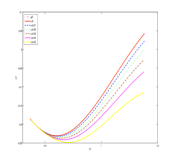
Refer to caption
(a) Hugoniot curves (projection onto the plane h1q1subscript1subscript𝑞1h_{1}-q_{1})
Refer to caption
(b) Hugoniot curves (projection onto the plane h2q2subscript2subscript𝑞2h_{2}-q_{2})
Figure 14: Test case 5.4. Hugoniot curves: ϵ{0.0, 0.01, 0.02, 0.03, 0.04, 0.05}italic-ϵ0.00.010.020.030.040.05\epsilon\in\left\{0.0,\ 0.01,\ 0.02,\ 0.03,\ 0.04,\ 0.05\right\}.

Next, we consider the Lax-Friedrichs schemes related to the new choice of the family of paths. An easy calculation shows again that, for this new family of paths, the last term of the modified equation (3.1) also vanishes. As a consequence, the second order modified equation is independent of ϵitalic-ϵ\epsilon: it coincides with the one corresponding to the family of segments.

We proceed as in the previous test case to compute the Hugoniot curves corresponding to the numerical scheme. In Figure 15 the curves obtained using a mesh with step Δx=0.001Δ𝑥0.001\Delta x=0.001 for ϵitalic-ϵ\epsilon = 0.00, 0.01, 0.02, 0.03, 0.04, 0.05, are depicted. Observe that all of the curves coincide: the Hugoniot curves obtained with the Lax-Friedrichs scheme for the different values of ϵitalic-ϵ\epsilon are reparameterizations of the same curve. This fact agrees with the fact that the second order modified equation is independent of ϵitalic-ϵ\epsilon.

Refer to caption
(a) Hugoniot curves (projection onto the plane h1q1subscript1subscript𝑞1h_{1}-q_{1})
Refer to caption
(b) Hugoniot curves (projection onto the plane h2q2subscript2subscript𝑞2h_{2}-q_{2})
Figure 15: Test case 5.4. Hugoniot curves for Lax-Friedrichs scheme with ϵ{0.0, 0.01, 0.02, 0.03, 0.04, 0.05}italic-ϵ0.00.010.020.030.040.05\epsilon\in\left\{0.0,\ 0.01,\ 0.02,\ 0.03,\ 0.04,\ 0.05\right\}: exact (red lines) and numerical (lines with dots).

Figure 16 shows the projections of the Hugoniot curve corresponding to Roe scheme for ϵitalic-ϵ\epsilon = 0.00, 0.01, 0.02, 0.03, 0.04, 0.05 (line with dots) onto the planes h1q1subscript1subscript𝑞1h_{1}-q_{1} and h2q2subscript2subscript𝑞2h_{2}-q_{2}. Note that, in this case, the obtained curves depend on ϵitalic-ϵ\epsilon, but again the numerical solutions do not converge to the weak solutions corresponding to the chosen family of paths. Nevertheless, as in the previous test case, if wrsubscript𝑤𝑟w_{r} and wlsubscript𝑤𝑙w_{l} are close enough or the shock speed is close to zero, the exact and the numerical Hugoniot curves are also close.
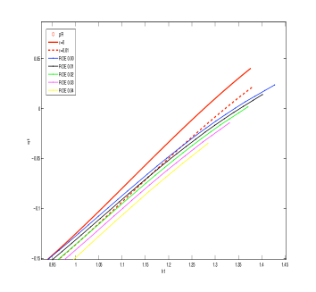
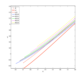
Refer to caption
(a) 3-shock hugoniot curves (projection onto the plane h1q1subscript1subscript𝑞1h_{1}-q_{1})
Refer to caption
(b) 3-shok hugoniot curves (projection onto the plane h2q2subscript2subscript𝑞2h_{2}-q_{2})
Figure 16: Test case 5.4. 3-shock hugoniot curves (zoom) for Roe scheme with ϵ{0.0, 0.01, 0.02, 0.03, 0.04, 0.05}italic-ϵ0.00.010.020.030.040.05\epsilon\in\left\{0.0,\ 0.01,\ 0.02,\ 0.03,\ 0.04,\ 0.05\right\}: exact (red lines) and numerical (lines with dots).

6 Conclusions

When a hyperbolic system with nonconservative products and genuinely nonlinear fields is discretized, in order to be sure that the numerical approximations converge to a function which is a classical solution where it is smooth and whose discontinuities are in good agreement with the physics of the problem, the following steps should be taken [19, 16]:

  • First, choose a regularization of the system which is consistent with the physics of the problem.

  • Next, determine the DLM family of paths consistent with this regularization.

  • Finally, design a numerical scheme whose solutions converge to weak solutions associated with this family of paths.

In practice, this strategy may be difficult to follow, since the actual calculation of a family of paths requires calculating regularized shock profiles associated with the given regularization. On the other hand, the convergence of the numerical solutions to the correct weak solutions is known for the Glimm scheme and the front tracking method [24], only; the implementation of these methods can be time consuming since they require the explicit knowledge of the corresponding Riemann solver.

In fact, when the nonconservative model under consideration is a simplified version of a more complex (but conservative) model —as is the case for the two-layer shallow water system— the above strategy may end up being more costly than than solving directly the more complex one. In these cases, the use of a numerical strategy based on a direct discretization of the nonconservative system by means of finite difference scheme which is formally path-consistent is advisable and may have the following advantages:

  • The numerical solutions is formally consistent with the definition of the nonconservative product in the sense of Dal Maso, LeFloch, and Murat and, in turn, in the special case that the system admits a conservative subsystem, the numerical scheme is conservative for that subsystem in the sense of Lax.

  • The approximations of the shocks provided by the schemes are consistent with a regularization of the system with higher-order terms that vanish as ΔxΔ𝑥\Delta x tends to 0. (Obviously, the main drawback is that this regularization depends on the chosen family of paths and on the numerical scheme itself. This is issue dealt with in the present paper.)

  • As originally pointed out by Hou and LeFloch [16] in the (simpler) case of scalar hyperbolic equations, the convergence error, measured in terms of our convergence error measure or in terms of the Hugoniot curves, is noticeable for very fine meshes, for discontinuities of great amplitude, and/or for large-time simulations, only.

  • This strategy is extendable to high-order methods or to multidimensional problems, as developed, together with collaborators, by Coquel [1, 2, 11] and Pares [5, 6].

The convergence error should also be compared with the experimental error. In the case of the two-layer shallow water system, the shocks captured by Roe scheme and the family of straightlines have been found [7] to be in good agreement with the experimental measurements of internal bores in the Strait of Gibraltar, despite of the simplicity of the family of paths.

In certain special situations, the convergence error measure is found to vanish identically. This is the case of systems whose nonconservative product is associated with a linearly degenerate field: for schemes that are formally consistent with a family of paths satisfying the condition (R1), then all of the discontinuities are correctly approximated and the scheme does converge to exact solutions. The discussion of linearly degenerate fields associated with nonconservative products was discussed earlier in [19, 26] from the theoretical standpoint and in [4] from the numerical standpoint. This problem may also exhibit an additional difficulty, the resonance problem, if one of the eigenvalues of the Jacobian matrix vanishes, and weak solutions may not be uniquely determined by their initial data, so that the limiting numerical solutions may depend both on the family of paths and the numerical scheme itself.

Acknowledgments

This research was partially supported by the Spanish Government Research project MTM2006-08075, by the A.N.R. (Agence Nationale de la Recherche) through the grant 06-2-134423, and by the Centre National de la Recherche Scientifique (CNRS). The authors are grateful to Frédéric Coquel for discussions on the matter of this paper.

References

  • [1] C. Berthon and F. Coquel, Nonlinear projection methods for multi-entropies Navier-Stokes systems, in ”Innovative methods for numerical solutions of partial differential equations” (Arcachon, 1998), pp. 278–304, World Sci. Publ., River Edge, NJ, 2002.
  • [2] C. Berthon and F. Coquel, Nonlinear projection methods for multi-entropies Navier-Stokes systems, Math. of Comp. 76 (2007), 1163–1194.
  • [3] C. Berthon, F. Coquel, and P.G. LeFloch, Why many theories of shock waves are necessary. Kinetic relations for nonconservative systems, in preparation.
  • [4] F. Bouchut, Nonlinear stability of finite volume methods for hyperbolic conservation laws and well-balanced schemes for sources, Frontiers in Math., Birkh user Verlag, Bäsel, 2004.
  • [5] M.J. Castro, J.M. Gallardo, and C. Parés, High-order finite volume schemes based on reconstruction of states for solving hyperbolic systems with nonconservative products. Applications to shallow-water systems, Math. of Comp. 75 (2006), 1103–1134.
  • [6] M.J. Castro, J.M. Gallardo, and C. Parés, On a well-balanced high-order finite volume scheme for shallow water equations with topography and dry areas, J. Comput. Phys. 227 (2007), 574–601.
  • [7] M.J. Castro, J.A. García, J.M. González, J. Macías, C. Parés, and M.E. Vázquez, Numerical simulation of two layer shallow water flows through channels with irregular geometry, J. Comput. Phys. 195 (2004), 202–235.
  • [8] M.J. Castro, J. Macías, and C. Parés, A Q𝑄Q-Scheme for a class of systems of coupled conservation laws with source term. Application to a two-layer 1-D shallow water system, Math. Mod. Num. Anal. 35 (2001), 107–127.
  • [9] M.J. Castro, A. Pardo, and C. Parés, Well-balanced numerical schemes based on a generalized hydrostatic reconstruction technique, Math. Mod. Meth. App. Sci. 17 (2007), 2055–2113.
  • [10] M.J. Castro, A. Pardo, C. Parés, and E.F. Toro, Coefficient-splitting numerical schemes for nonconservative hyperbolic systems and high order extensions, in preparation.
  • [11] C. Chalons and F. Coquel, Numerical capture of shock solutions of nonconservative hyperbolic systems via kinetic functions. Analysis and simulation of fluid dynamics, Adv. Math. Fluid Mech., pp. 45–68, Birkhäuser, Bäsel, 2007.
  • [12] R. Courant and K.O. Friedrichs, Supersonic flow and shock waves, John Wiley, New York, 1948.
  • [13] G. Dal Maso, P.G. LeFloch, and F. Murat, Definition and weak stability of nonconservative products, J. Math. Pures Appl. 74 (1995), 483–548.
  • [14] B.T. Hayes and P.G. LeFloch, Nonclassical shocks and kinetic relations : scalar conservation laws, Arch. Rational Mech. Anal. 139 (1997), 1–56.
  • [15] B.T. Hayes and P.G. LeFloch, Nonclassical shocks and kinetic relations: finite difference schemes, SIAM J. Numer. Anal. 35 (1998), 2169–2194.
  • [16] T.Y. Hou and P.G. LeFloch, Why nonconservative schemes converge to wrong solutions: error analysis, Math. of Comput. 62 (1994), 497–530.
  • [17] P.D. Lax and B. Wendroff, Systems of conservation laws, Comm. Pure Appl. Math. 13 (1960), 217–237.
  • [18] P.G. LeFloch, Entropy weak solutions to nonlinear hyperbolic systems in nonconservative form, Comm. Part. Diff. Equa. 13 (1988), 669–727.
  • [19] P.G. LeFloch, Shock waves for nonlinear hyperbolic systems in nonconservative form, Institute for Math. and its Appl., Minneapolis, Preprint # 593, 1989.
  • [20] P.G. LeFloch, Entropy weak solutions to nonlinear hyperbolic systems in conservative form, Proc. Intern. Conf. on Hyperbolic problems, ed. J. Ballmann and R. Jeltsch, Note on Num. Fluid Mech., Vol. 24, Viewieg, Braunschweig, 1989, pp. 362–373.
  • [21] P.G. LeFloch, On some nonlinear hyperbolic problems (in English), Habilitation à Diriger des Recherches, Université de Paris 6, 1990.
  • [22] P.G. LeFloch, Hyperbolic systems of conservation laws: The theory of classical and nonclassical shock waves, Lectures in Mathematics, ETH Zürich, Birkhäuser, 2002.
  • [23] P.G. LeFloch, Graph solutions of nonlinear hyperbolic systems, J. Hyper. Diff. Equa. 1 (2004), 643–689.
  • [24] P.G. LeFloch and T.-P. Liu, Existence theory for nonlinear hyperbolic systems in nonconservative form, Forum Math. 5 (1993), 261–280.
  • [25] P.G. LeFloch and M. Mohamadian, Why many shock wave theories are necessary. Fourth-order models, kinetic functions, and equivalent equations, J. Comput. Phys. 227 (2008), 4162–4189.
  • [26] P.G. LeFloch and M.D. Thanh, The Riemann problem for fluid flows in a nozzle with discontinuous cross-section, Comm. Math. Sci. 1 (2003), 763–796.
  • [27] P.G. LeFloch and M.D. Thanh, The Riemann problem for the shallow water equations with discontinuous topography, Comm. Math. Sc. 5 (2007), 865–885.
  • [28] M.L. Muñoz-Ruiz and C. Parés, Godunov method for nonconservative hyperbolic systems, Math. Method. Anal. Num. 41 (2007), 169–185.
  • [29] S. Noelle, Y. Xing, and C.W. Shu, High-order well-balanced finite volume WENO schemes for shallow water equation with moving water, J. Comput. Phys. 226 (2007), 29–58.
  • [30] C. Parés, Numerical methods for nonconservative hyperbolic systems: a theoretical framework, SIAM J. Numer. Anal. 44 (2006), 300–321.
  • [31] C. Parés and M.J. Castro, On the well-balance property of Roe’s method for nonconservative hyperbolic systems. Applications to shallow-water systems, Math. Model. Numer. Anal. 38 (2004), 821–852.
  • [32] J.B. Schijf and J.C. Schonfeld, Theoretical considerations on the motion of salt and fresh water, in Proc. Minn. Int. Hydraulics Conv., joint meeting IAHR Hydro. Div. ASCE. (Sept. 1953) 1953, pp. 321–333.
  • [33] Y. Xing and C.-W. Shu, High order well-balanced finite volume WENO schemes and discontinuous Galerkin methods for a class of hyperbolic systems with source terms, J. Comput. Phys. 214 (2006), 567–598.