Symmetries in collective neutrino oscillations

Abstract

We discuss the relationship between a symmetry in the neutrino flavour evolution equations and neutrino flavour oscillations in the collective precession mode. This collective precession mode can give rise to spectral swaps (splits) when conditions can be approximated as homogeneous and isotropic. Multi-angle numerical simulations of supernova neutrino flavour transformation show that when this approximation breaks down, non-collective neutrino oscillation modes decohere kinematically, but the collective precession mode still is expected to stand out. We provide a criterion for significant flavour transformation to occur if neutrinos participate in a collective precession mode. This criterion can be used to understand the suppression of collective neutrino oscillations in anisotropic environments in the presence of a high matter density. This criterion is also useful in understanding the breakdown of the collective precession mode when neutrino densities are small.

1 Introduction

Because of neutrino-neutrino forward scattering or neutrino self-interaction [1, 2, 3] neutrinos can experience collective flavour transformation in environments such as the early Universe (e.g., [4, 5, 6, 7, 8, 9]) and supernovae (e.g., [10, 11, 12, 13]) where neutrino number densities can be very large. This phenomenon is different from the conventional Mikheyev-Smirnov-Wolfenstein (MSW) effect [14, 15] in that the flavour evolution histories of neutrinos in collective oscillations are coupled together and must be solved simultaneously. The possibility and consequences of collective neutrino oscillations in supernovae were not well appreciated until the discovery that the ordinary matter can be “ignored” in such phenomena [16] and the first numerical demonstrations of “stepwise spectral swapping” (or “spectral split”) [17, 18] which is the imprint left by the collective flavour transformation on neutrino energy spectra.

Significant progress has been made towards understanding collective neutrino oscillations in supernovae (see, e.g., [19] for a brief review and references therein). In particular, Raffelt and Smirnov [20] demonstrated an adiabatic (precession) solution for the homogeneous, isotropic neutrino gas. This solution has been shown to agree in part with the results of “single-angle” simulations of supernova neutrino oscillations [21]. These single-angle simulations essentially neglect the anisotropic nature of the supernova environment by assuming that the flavour evolution histories of neutrinos along all trajectories are identical to those along a “representative” trajectory, usually taken to be the radial trajectory [10, 22]. The adiabatic precession solution requires that at any time all neutrinos reside in a pure collective oscillation mode, the “precession” mode, which, as shown by Duan et al[18, 23], would explain the spectral swap phenomenon in the single-angle simulations.

However, the real supernova environment is highly inhomogeneous and anisotropic. Here by “inhomogeneous” and “anisotropic” we are referring to the neutrino fields. Of course, the matter density distributions in the supernova environment are also likely to be inhomogeneous and anisotropic. To date there are a few “multi-angle” simulations [17, 18, 24, 25] which, like the single-angle calculations, also adopt spherically symmetric supernova models but do treat flavour evolution along different neutrino trajectories in a self-consistent way. These multi-angle calculations also exhibit spectral swaps. It is still not understood how the spectral swap phenomenon arises in the (anisotropic) multi-angle context. In fact, some studies seem to suggest that collective neutrino oscillations in the isotropic and anisotropic environments can be very different. For example, collective neutrino oscillations of the bipolar type can experience “kinematic decoherence” and be disrupted in anisotropic environments [26, 27]. Additionally, a very large matter background can result in neutrino oscillation phase differences between different neutrino trajectories in an anisotropic neutrino gas [10], and this effect recently has been shown to result in suppression of collective neutrino oscillations [28].

In this paper we discuss a SU($N_{\mathrm{f}}$) rotation symmetry in the neutrino flavour evolution equations, where $N_{\mathrm{f}}=2$ and 3 for the two-flavour and three-flavour neutrino mixing schemes, respectively. The collective precession mode for neutrino oscillations can ensue from this symmetry, even in inhomogeneous, anisotropic environments. This result explains the puzzling observations of the spectral swapping phenomenon in both the single-angle and multi-angle simulations of supernova neutrino oscillations.

The rest of this paper is organized as follows. In section 2 we lay out the general framework for neutrino flavour transformation and discuss the SU($N_{\mathrm{f}}$) rotation symmetry in the flavour evolution equations for a dense neutrino gas. In section 3 we show how the collective precession mode for neutrino oscillations can arise from this symmetry in various environments. We also give criteria for when the collection precession mode can occur. In section 4 we present a new multi-angle simulation of supernova neutrino oscillations. We analyze the results of this calculation guided by our understanding of the collective precession mode. In section 5 we give our conclusions.

2 Equations of motion and symmetries

2.1 Neutrino flavour polarization matrix

We are interested in collective flavour oscillations in neutrino gases in which neutrinos may experience only forward scattering on other particles (including other neutrinos), but where no inelastic scattering occurs. When physical conditions change only slowly with spatial dimension, the flavour content of neutrinos can be described by semi-classical matrices of densities [29, 30]

$$\left[\rho{p}(t,\bi{x})\right]_{\alpha\beta} =\sum n_{\nu,\bi{p}}(t,\bi{x})\langle\nu_{\alpha}|\psi_{\nu,\bi{p}}(t,\bi{x})\rangle\langle\psi_{\nu,\bi{p}}(t,\bi{x})|\nu_{\beta}\rangle,$$ (1)

$$\left[\bar{\rho}{p}(t,\bi{x})\right]_{\alpha\beta} =\sum n_{\bar{\nu},\bi{p}}(t,\bi{x})\langle\bar{\nu}_{\beta}|\psi_{\bar{\nu},\bi{p}}(t,\bi{x})\rangle\langle\psi_{\bar{\nu},\bi{p}}(t,\bi{x})|\bar{\nu}_{\alpha}\rangle,$$ (2)

where $\alpha$ and $\beta$ are flavour labels ($e$, $\mu$, $\tau$), $|\psi_{\nu(\bar{\nu}),\bi{p}}(t,\bi{x})\rangle$ is the state of a neutrino $\nu$ (antineutrino $\bar{\nu}$) with momentum $\bi{p}$ at time $t$ and position $\bi{x}$, $n_{\nu(\bar{\nu}),\bi{p}}$ is the corresponding neutrino number density, and the summation runs over all neutrino (antineutrino) states. Matrices of densities defined in (1) and (2) contain two separate pieces of information. One is the overall number density of neutrinos or antineutrinos with momentum $\bi{p}$ at spacetime point $(t,\bi{x})$:

$$n_{p}(t,\bi{x})\equiv\left\{\begin{array}[]{ll}\Tr\rho{p}(t,\bi{x})&\textrm{ if }p^{0}>0,\\ \Tr\bar{\rho}{p}(t,\bi{x})&\textrm{ if }p^{0}<0.\end{array}\right.$$ (3)

Here for compactness we use 4-component vector $p\equiv[p^{0},\bi{p}]$ to denote a neutrino or antineutrino momentum mode, where $p^{0}=|\bi{p}|$ for the neutrino and $-|\bi{p}|$ for the antineutrino. Because neutrinos may experience only forward scattering, $n_{p}(t,\bi{x})$ satisfies the conservation equation

$$(\partial_{t}+\hat{\bi{p}}\cdot\boldsymbol{\nabla})n_{p}(t,\bi{x})=0,$$ (4)

where $\hat{\bi{p}}\equiv\bi{p}/|\bi{p}|$ is the unit vector along the neutrino propagation direction.

The other piece of information contained in the matrix of density is the “flavour polarization” of the neutrino. This is in analogy to, e.g., the spin polarization of an electron gas. We define a traceless “neutrino flavour polarization matrix”, or “polarization matrix” for short,

$$\mathsf{P}_{p}(t,\bi{x})\equiv\left\{\begin{array}[]{ll}n_{p}^{-1}(t,\bi{x})\rho_{p}(t,\bi{x})-N_{\mathrm{f}}^{-1}\mathsf{I}&\textrm{ if }p^{0}>0,\\ -n_{p}^{-1}(t,\bi{x})\rho_{p}(t,\bi{x})+N_{\mathrm{f}}^{-1}\mathsf{I}&\textrm{ if }p^{0}<0,\end{array}\right.$$ (5)

where $\mathsf{I}$ is the identity matrix in flavour space, and $N_{\mathrm{f}}=2$ and 3 for two-flavour and three-flavour mixing schemes, respectively. In (5) we define the polarization matrices for neutrinos and antineutrinos with opposite signs, with the understanding that antiparticles are “negative particles” or “holes” in the particle sea. This sign convention will make the equations of motion (e.o.m.) more succinct and is especially appropriate in the two-flavour mixing scheme where $\mathbf{2}$ and $\bar{\mathbf{2}}$, the fundamental representations of the SU(2) group, are equivalent [16] (see section 2.2). The e.o.m. for polarization matrix $\mathsf{P}_{p}(t,\bi{x})$ can be derived easily from that for $\rho_{p}(t,\bi{x})$ [29, 30, 31] and is

$$(\partial_{t}+\hat{\bi{p}}\cdot\boldsymbol{\nabla})\mathsf{P}_{p}(t,\bi{x})=-\rmi[\mathsf{H}_{p}(t,\bi{x}),\mathsf{P}_{p}(t,\bi{x})].$$ (6)

Throughout this paper we assume a vanishing $CP$-violating phase. (See [32] for a discussion of collective neutrino oscillations with a non-vanishing $CP$-violating phase.)

The Hamiltonian for polarization matrix $\mathsf{P}_{p}(t,\bi{x})$ is

$$\mathsf{H}_{p}(t,\bi{x}) =\mathsf{H}_{p^{0}}^{\mathrm{ext}}(t,\bi{x})+\mathsf{H}_{\hat{\bi{p}}}^{\nu\nu}(n_{p^{\prime}}(t,\bi{x}),\mathsf{P}_{p^{\prime}}(t,\bi{x})|\forall p^{\prime}),$$ (7)

$$=\mathsf{H}_{p^{0}}^{\mathrm{vac}}+\mathsf{H}^{\mathrm{matt}}(t,\bi{x})+\mathsf{H}_{\hat{\bi{p}}}^{\nu\nu}(n_{p^{\prime}}(t,\bi{x}),\mathsf{P}_{p^{\prime}}(t,\bi{x})|\forall p^{\prime}).$$

The background “neutrino field”

$$\mathsf{H}_{\hat{\bi{p}}}^{\nu\nu}(n_{p^{\prime}}(t,\bi{x}),\mathsf{P}_{p^{\prime}}(t,\bi{x})|\forall p^{\prime})=\sqrt{2}G_{\mathrm{F}}\sum_{p^{\prime}}(1-\hat{\bi{p}}\cdot\hat{\bi{p}}^{\prime})n_{p^{\prime}}(t,\bi{x})\mathsf{P}_{p^{\prime}}(t,\bi{x})$$ (8)

is a function of both neutrino number densities $n_{p^{\prime}}(t,\bi{x})$ and neutrino flavour polarization matrices $\mathsf{P}_{p^{\prime}}(t,\bi{x})$, and does not depend on the energy of the test neutrino. For convenience we will drop the symbol “$\forall p^{\prime}$” with the understanding that $p^{\prime}$ in $\mathsf{H}_{\hat{\bi{p}}}^{\nu\nu}(n_{p^{\prime}}(t,\bi{x}),\mathsf{P}_{p^{\prime}}(t,\bi{x}))$ refers to all neutrino modes. In (8) we use $\sum_{p^{\prime}}$ to denote the integration over $(p^{\prime})^{0}$ and $\hat{\bi{p}}^{\prime}$:

$$\sum_{p^{\prime}}\equiv\int_{-\infty}^{\infty}\rmd(p^{\prime})^{0}\int\!\rmd\hat{\bi{p}}^{\prime}.$$ (9)

The procedure implied in equation (9) is tantamount to a sum over neutrino and antineutrino energies and trajectory directions. The “vacuum field”

$$\mathsf{H}_{p^{0}}^{\mathrm{vac}}=\frac{\mathsf{M}^{2}}{2p^{0}}$$ (10)

generates vacuum oscillations, where $\mathsf{M}$ is the neutrino mass matrix. Because the trace of a Hamiltonian has no effect on neutrino oscillations, we will take $\mathsf{H}_{p^{0}}^{\mathrm{vac}}$ to be traceless hereafter. With this convention (10) in the vacuum mass basis becomes

$$\mathsf{H}_{p^{0}}^{\mathrm{vac}}=-\frac{\Delta m^{2}_{21}}{2p^{0}}\frac{\Lambda_{3}}{2}-\left(\frac{\Delta m^{2}_{31}+\Delta m^{2}_{32}}{4p^{0}}\right)\frac{\Lambda_{8}}{\sqrt{3}},$$ (11)

where $\Delta m^{2}_{ij}=m_{i}^{2}-m_{j}^{2}$ is the difference between the squares of the mass eigenvalues corresponding to mass eigenstates $|\nu_{i}\rangle$ and $|\nu_{j}\rangle,$ and $\Lambda_{a}$ ($a=1,2,\ldots,8$) are the Gell-Mann matrices. For the two-flavour mixing scheme

$$\mathsf{H}_{p^{0}}^{\mathrm{vac}}=-\frac{\Delta m^{2}}{2p^{0}}\frac{\Lambda_{3}}{2},$$ (12)

where $\Lambda_{3}$ is the third Pauli matrix. The $2\times 2$ case is analogous to the $3\times 3$ case discussed above except $\Lambda_{a}$ ($a=1,2,3$) are the Pauli matrices. The “matter field” in the flavour basis in the supernova environment is

$$\mathsf{H}^{\mathrm{matt}}(t,\bi{x})=\lambda(t,\bi{x})\,\mathrm{diag}[1,0,0]=\sqrt{2}G_{\mathrm{F}}n_{e}(t,\bi{x})\,\mathrm{diag}[1,0,0],$$ (13)

where $G_{\mathrm{F}}$ is the Fermi constant, and $n_{e}(t,\bi{x})$ is the net electron number density. The vacuum field $\mathsf{H}_{p^{0}}^{\mathrm{vac}}$ and the matter field $\mathsf{H}^{\mathrm{matt}}(t,\bi{x})$ together constitute the total external field, $\mathsf{H}^{\mathrm{ext}}_{p^{0}}(t,\bi{x})$, which does not depend on neutrino flavours.

2.2 Vector representation of the polarization matrix

An $N_{\mathrm{f}}\times N_{\mathrm{f}}$, traceless, Hermitian matrix $\mathsf{A}$ can be written in terms of vector $\vec{A}$ as

$$\mathsf{A}=\frac{\vec{\Lambda}}{2}\cdot\vec{A}\equiv\sum_{a}\frac{\Lambda_{a}}{2}A_{a}.$$ (14)

(We have adopted the convention in [22]. We use bold-faced letters, e.g., $\bi{A}$ to denote 3-vectors in coordinate space, sans-serif letters, e.g., $\mathsf{A}$ for matrices in flavour space, and letters with an arrow, e.g., $\vec{A}$ for vectors in flavour space.) The e.o.m. for the “polarization vector” $\vec{P}_{p}(t,\bi{x})$ is [33]

$$(\partial_{t}+\hat{\bi{p}}\cdot\boldsymbol{\nabla})\vec{P}_{p}(t,\bi{x})=\vec{H}_{p}(t,\bi{x})\times\vec{P}_{p}(t,\bi{x}),$$ (15)

where the cross product between two vectors is defined by the structure constants $f_{abc}$ of the SU($N_{\mathrm{f}}$) group [34]:

$$(\vec{A}\times\vec{B})_{a}\equiv f_{abc}A_{b}B_{c}.$$ (16)

The definition of the polarization vector $\vec{P}_{p}$ given by (5) and (14) for the antineutrino has a different sign as compared with that in [29] and with the 8-dimensional Bloch vector in [33]. In addition to making the expression of $\vec{H}^{\nu\nu}_{\hat{\bi{p}}}(t,\bi{x})$ [see (8)] more compact, this convention is especially convenient in the two-flavour mixing scheme. In studying collective neutrino oscillations the corotating-frame transformation technique [16] is frequently used. A corotating-frame transformation corresponds to rewriting (15) in a reference frame that rotates about $\vec{e}_{3}$ with angular frequency $\omega_{0}$, where $\vec{e}_{3}$ is the unit basis vector corresponding to $\Lambda_{3}$ in the vacuum mass basis. According to (7) and (10) this transformation is equivalent to a change in the momentum of the neutrino $p\rightarrow p^{\prime}$ where

$$\frac{\delta m^{2}}{2(p^{\prime})^{0}}=\frac{\delta m^{2}}{2p^{0}}-\omega_{0}\quad\textrm{and}\quad\hat{\bi{p}}^{\prime}=\hat{\bi{p}}.$$ (17)

With the traditional definition, the direction of the polarization vector $\vec{P}_{p}$ must be reversed when $p^{0}$ changes sign under the transformation (17). The polarization vector defined by (5) and (14), however, is invariant under such transformations. This definition has already been adopted in some recent literature, e.g., [35].

We can define the magnitude of $\mathsf{P}_{p}$ as

$$|\mathsf{P}_{p}|\equiv|\vec{P}_{p}|\equiv\sqrt{\sum_{a}P_{a}^{2}}\leq\sqrt{\frac{2}{N_{\mathrm{f}}}(N_{\mathrm{f}}-1)}.$$ (18)

The equal sign in the above strict inequality relation applies only if the neutrino state is a pure (quantum) state, i.e., can be described by a single ket. In forward-scattering the coherence of the neutrino is not lost and, therefore, $|\mathsf{P}_{p}(t,\bi{x})|$ also obeys the conservation equation

$$(\partial_{t}+\hat{\bi{p}}\cdot\boldsymbol{\nabla})|\mathsf{P}_{p}(t,\bi{x})|=0.$$ (19)

In the two-flavour mixing scheme a notation related to the polarization vector is the neutrino flavour isospin (NFIS) [16]. It can be defined as

$$\vec{s}_{p}(t,\bi{x})\equiv\frac{\vec{P}(t,\bi{x})}{2|\vec{P}(t,\bi{x})|}$$ (20)

if the neutrino state is a pure state. It obeys the e.o.m.

$$(\partial_{t}+\hat{\bi{p}}\cdot\boldsymbol{\nabla})\vec{s}_{p}(t,\bi{x}) =\vec{s}_{p}(t,\bi{x})\times[-\vec{H}^{\mathrm{vac}}_{p^{0}}-\vec{H}^{\mathrm{matt}}(t,\bi{x})$$ (21)

$$\quad-2\sqrt{2}G_{\mathrm{F}}\sum_{p^{\prime}}(1-\hat{\bi{p}}\cdot\hat{\bi{p}}^{\prime})n_{p^{\prime}}(t,\bi{x})\vec{s}_{p^{\prime}}(t,\bi{x})].$$

Equation (21) shows that two NFIS’s $\vec{s}_{p}(t,\bi{x})$ and $\vec{s}_{p^{\prime}}(t,\bi{x})$ at the same space-time point are “antiferromagnetically” coupled. Note that we have defined Hamiltonian vector fields in the same way as [20] but differing by a minus sign from those in the original NFIS notation [16]. In supernovae the neutrinos in a given momentum mode usually are not in a pure state. Assuming that supernova neutrinos are emitted in pure flavour states at the neutrino sphere and subsequently encounter only forward-scattering, we can write

$$n_{p}(t,\bi{x})\vec{P}_{p}(t,\bi{x})=2\sum_{\alpha}n_{\alpha,p}(t,\bi{x})\vec{s}_{\alpha,p}(t,\bi{x}).$$ (22)

In (22) $\vec{s}_{\alpha,p}(t,\bi{x})$ is the NFIS that represents the flavour state of the neutrino or antineutrino at $(t,\bi{x})$ which is pure $\nu_{\alpha}$ or $\bar{\nu}_{\alpha}$ at the neutrino sphere, and $n_{\alpha,p}(t,\bi{x})$ is the associated neutrino number density. The corresponding replacements in (21) are

$$\vec{s}_{p}\rightarrow\vec{s}_{\alpha,p},\quad\vec{s}_{p^{\prime}}\rightarrow\vec{s}_{\alpha^{\prime},p^{\prime}},\quad n_{p^{\prime}}\rightarrow n_{\alpha^{\prime},p^{\prime}}\quad\textrm{and}\quad\sum_{p^{\prime}}\rightarrow\sum_{\alpha^{\prime},p^{\prime}}.$$

Equivalently, we can insist on the definition (20) and replace $n_{p}(t,\bi{x})$ in (21) by

$$n_{p}^{\prime}(t,\bi{x})\equiv n_{p}(t,\bi{x})|\vec{P}(t,\bi{x})|.$$ (23)

In the latter approach, NFIS $\vec{s}_{p}(t,\bi{x})$ represents the “average flavour state” of the neutrino, and $n_{p}^{\prime}(t,\bi{x})$ is the “net number density” of the neutrino in the flavour state represented by $\vec{s}_{p}(t,\bi{x})$.

2.3 Symmetries and conservation laws

From (8) it is easy to show that $\mathsf{H}_{\hat{\bi{p}}}^{\nu\nu}(n_{p^{\prime}}(t,\bi{x}),\mathsf{P}_{p^{\prime}}(t,\bi{x}))$ satisfies two important identities:

$$\sum_{p}n_{p}(t,\bi{x})[\mathsf{P}_{p}(t,\bi{x}),\mathsf{H}_{\hat{\bi{p}}}^{\nu\nu}(n_{p^{\prime}}(t,\bi{x}),\mathsf{P}_{p^{\prime}}(t,\bi{x}))]=0;$$ (24)

and

$$\mathsf{U}(t,\bi{x})\mathsf{H}_{\hat{\bi{p}}}^{\nu\nu}(n_{p^{\prime}}(t,\bi{x}),\mathsf{P}_{p^{\prime}}(t,\bi{x}))\mathsf{U}^{\dagger}(t,\bi{x})=\mathsf{H}_{\hat{\bi{p}}}^{\nu\nu}(n_{p^{\prime}}(t,\bi{x}),\mathsf{U}(t,\bi{x})\mathsf{P}_{p^{\prime}}(t,\bi{x})\mathsf{U}^{\dagger}(t,\bi{x})),$$ (25)

where $\mathsf{U}(t,\bi{x})$ is an arbitrary unitary matrix.

Equation (24) implies that, if

$$[\mathsf{G},\mathsf{H}_{p^{0}}^{\mathrm{ext}}(t,\bi{x})]=0,$$ (26)

where $\mathsf{G}$ is a constant $N_{\mathrm{f}}\times N_{\mathrm{f}}$ traceless Hermitian matrix, then the lepton current $L^{\mu}(t,\bi{x})$ with temporal and spatial components

$$L^{0}(t,\bi{x}) \equiv\sum_{p}n_{p}(t,\bi{x})\Tr\left[\mathsf{P}_{p}(t,\bi{x})\,\mathsf{G}\right],$$ (27)

$$\bi{L}(t,\bi{x}) \equiv\sum_{p}\hat{\bi{p}}\,n_{p}(t,\bi{x})\Tr\left[\mathsf{P}_{p}(t,\bi{x})\,\mathsf{G}\right]$$ (28)

satisfies the continuity equation

$$\partial_{\mu}L^{\mu}(t,\bi{x})=\partial_{t}L^{0}(t,\bi{x})+\boldsymbol{\nabla}\cdot\bi{L}(t,\bi{x})=0.$$ (29)

This can be easily shown using (4), (6), (7), (24) and (26):

$$\partial_{\mu}L^{\mu}(t,\bi{x}) =\rmi\sum_{p}n_{p}(t,\bi{x})\Tr\left([\mathsf{P}_{p}(t,\bi{x}),\mathsf{H}_{p}(t,\bi{x})]\,\mathsf{G}\right)$$ (30)

$$=\rmi\sum_{p}n_{p}(t,\bi{x})\Tr\left([\mathsf{P}_{p}(t,\bi{x}),\mathsf{H}_{p^{0}}^{\mathrm{ext}}(t,\bi{x})]\,\mathsf{G}\right)$$

$$=\rmi\sum_{p}n_{p}(t,\bi{x})\Tr\left(\mathsf{P}_{p}(t,\bi{x})\,[\mathsf{H}_{p^{0}}^{\mathrm{ext}}(t,\bi{x}),\mathsf{G}]\right)=0.$$

Equation (25) implies that, if (26) is true, then the e.o.m. (6) for the polarization matrix is invariant under the global (i.e., independent of $p$, $t$ and $\bi{x}$) SU($N_{\mathrm{f}}$) transformation

$$\mathsf{P}_{p}(t,\bi{x})\longrightarrow\tilde{\mathsf{P}}_{p}(t,\bi{x})\equiv\exp(-\rmi\phi\mathsf{G})\mathsf{P}_{p}(t,\bi{x})\exp(\rmi\phi\mathsf{G}),$$ (31)

where $\phi$ is an arbitrary constant scalar. This is because (26) implies

$$\exp(-\rmi\phi\mathsf{G})\mathsf{H}_{p^{0}}^{\mathrm{ext}}(t,\bi{x})\exp(\rmi\phi\mathsf{G})=\mathsf{H}_{p^{0}}^{\mathrm{ext}}(t,\bi{x}).$$ (32)

Using (6), (25) and (32) it can be shown that

$$(\partial_{t}+\hat{\bi{p}}\cdot\boldsymbol{\nabla})\tilde{\mathsf{P}}_{p}(t,\bi{x})=-\rmi\left[\mathsf{H}^{\mathrm{ext}}_{p^{0}}(t,\bi{x})+\mathsf{H}^{\nu\nu}_{\hat{\bi{p}}}(n_{p^{\prime}}(t,\bi{x}),\tilde{\mathsf{P}}_{p^{\prime}}(t,\bi{x})),\,\tilde{\mathsf{P}}_{p}(t,\bi{x})\right].$$ (33)

In the two-flavour mixing scheme it is obvious that $\Lambda_{3}$ (in the vacuum mass basis) commutes with $\mathsf{H}_{p^{0}}^{\mathrm{ext}}=\mathsf{H}_{p^{0}}^{\mathrm{vac}}$ in (12) in the absence of ordinary matter. According to the above discussion, the e.o.m. (15) for all polarization vectors $\vec{P}_{p}(t,\bi{x})$ are invariant under simultaneous rotations about $\vec{e}_{3}$. In a homogeneous and isotropic neutrino gas a collective neutrino oscillation mode, which is represented by the collective precession of all polarization vectors about $\vec{e}_{3}$, can arise because of this symmetry [23, 21]. This precession mode of collective neutrino oscillations will ultimately cause the energy spectra of neutrinos with different flavours to be swapped at a critical energy $E^{\mathrm{s}}$, a phenomenon known as the “stepwise spectral swapping” [18]. Not surprisingly, the value of $E^{\mathrm{s}}$ is determined by the conserved lepton number $L^{0}$ associated with $\Lambda_{3}$ [36, 20]. Similar conclusions have also been drawn for homogeneous, isotropic neutrino gases in the three-flavour mixing scheme [37, 38].

Approximate symmetries and conservation laws can exist for scenarios where matter densities are large. Noting that $\mathsf{H}^{\mathrm{matt}}(t,\bi{x})$ is invariant under any rotation in the $\nu_{\mu}$–$\nu_{\tau}$ subspace, one can diagonalize the $\nu_{\mu}$–$\nu_{\tau}$ submatrix of $\mathsf{H}^{\mathrm{ext}}_{p^{0}}(t,\bi{x})$ by a rotation $(\nu_{e},\nu_{\mu},\nu_{\tau})\rightarrow(\nu_{e},\nu_{\mu^{\prime}},\nu_{\tau^{\prime}})$. In this new basis the external field is written as

$$\mathsf{H}_{p^{0}}^{\mathrm{ext}}(t,\bi{x}) =\frac{1}{2p^{0}}\left[\begin{array}[]{lll}m_{ee}^{2}+2\sqrt{2}p^{0}G_{\mathrm{F}}n_{e}(t,\bi{x})&m_{e\mu^{\prime}}^{2}&m_{e\tau^{\prime}}^{2}\\ m_{e\mu^{\prime}}^{2}&m_{\mu^{\prime}\mu^{\prime}}^{2}&0\\ m_{e\tau^{\prime}}^{2}&0&m_{\tau^{\prime}\tau^{\prime}}^{2}\end{array}\right]$$ (37)

$$\simeq\frac{1}{2p^{0}}\mathrm{diag}[m_{ee}^{2}+2\sqrt{2}p^{0}G_{\mathrm{F}}n_{e}(t,\bi{x}),\,m_{\mu^{\prime}\mu^{\prime}}^{2},\,m_{\tau^{\prime}\tau^{\prime}}^{2}],$$ (38)

which is approximately diagonalized for any neutrino mode $p$ if $G_{\mathrm{F}}n_{e}(t,\bi{x})\gg|\Delta m^{2}_{ij}/(2p^{0})|$ (e.g., [39]). The approximate symmetries of the neutrino system about $\Lambda_{3}$ and $\Lambda_{8}$, therefore, exist in the new basis $(\nu_{e},\nu_{\mu^{\prime}},\nu_{\tau^{\prime}})$ instead of the vacuum mass basis [37].

3 Collective precession mode for neutrino oscillations

In this section we discuss the collective precession mode in the two-flavour mixing scheme. This collective mode solution can arise in various environments because of the symmetry discussed in section 2.3. Generalization to the full three-flavour mixing scheme is straightforward when the polarization matrix representation is used [37].

3.1 Stationary, homogeneous and isotropic environments

First we shall use the symmetry viewpoint to discuss neutrino oscillations in the collective precession mode in stationary, homogeneous, isotropic environments. In such environments no physical quantity depends on the neutrino propagation direction $\hat{\bi{p}}$ and neither the external field $\mathsf{H}_{p^{0}}^{\mathrm{ext}}$ nor the neutrino number density $n_{p^{0}}$ varies with space or time. Also in this case, the polarization matrices $\mathsf{P}_{p^{0}}(t)$ are uniform and isotropic, which means the neutrino self-interaction potential

$$\mathsf{H}^{\nu\nu}(n_{(p^{\prime})^{0}},\mathsf{P}_{(p^{\prime})^{0}}(t))=\sqrt{2}G_{\mathrm{F}}\sum_{(p^{\prime})^{0}}n_{(p^{\prime})^{0}}\mathsf{P}_{(p^{\prime})^{0}}(t)$$ (39)

does not depend on the momentum of the test neutrino. Suppose that the set of variables $\{\Omega,\tilde{\mathsf{P}}_{p^{0}}|\forall p^{0}\}$ solve the following equations

$$\left[\mathsf{H}_{p^{0}}^{\mathrm{ext}}+\mathsf{H}^{\nu\nu}(n_{(p^{\prime})^{0}},\tilde{\mathsf{P}}_{(p^{\prime})^{0}})+\Omega\frac{\Lambda_{3}}{2},\tilde{\mathsf{P}}_{p^{0}}\right]=0,$$ (40)

$$\sum_{p^{0}}n_{p^{0}}\Tr\left(\tilde{\mathsf{P}}_{p^{0}}\Lambda_{3}\right)=L^{0},$$ (41)

where $\Omega$ is a scalar independent of $p^{0}$, $\tilde{\mathsf{P}}_{p^{0}}$ are traceless Hermitian matrices, and $L^{0}$ is a constant. Here we adopt the the vacuum mass basis $(\nu_{1},\nu_{2})$ if $\mathsf{H}^{\mathrm{matt}}(t)$ is negligible, and the flavour basis $(\nu_{e},\nu_{\mu^{\prime}})$ (which is also the matter basis) if $\mathsf{H}^{\mathrm{matt}}(t)$ is dominant. Therefore,

$$\mathsf{H}^{\mathrm{ext}}_{p^{0}}\simeq-(\omega_{p^{0}}-\lambda)\frac{\Lambda_{3}}{2}\simeq\left\{\begin{array}[]{ll}-\frac{\Delta m^{2}}{2p^{0}}\frac{\Lambda_{3}}{2}&\textrm{ if }\lambda\textrm{ is negligible,}\\ -\left(\frac{\Delta m^{\prime 2}}{2p^{0}}-\lambda\right)\frac{\Lambda_{3}}{2}&\textrm{ if }\lambda\textrm{ is very large,}\end{array}\right.$$ (42)

where $\Delta m^{\prime 2}=m_{\mu^{\prime}\mu^{\prime}}^{2}-m_{ee}^{2}$ [see (38)]. In either case we have

$$[\mathsf{H}_{p^{0}}^{\mathrm{ext}},\,\Lambda_{3}]=0.$$ (43)

Using (25), (40) and (43) we can show easily that

$$\mathsf{P}_{p^{0}}(t)=\exp\left[\rmi(\Omega t-\phi_{0})\frac{\Lambda_{3}}{2}\right]\tilde{\mathsf{P}}_{p^{0}}\exp\left[-\rmi(\Omega t-\phi_{0})\frac{\Lambda_{3}}{2}\right]$$ (44)

is a solution to the e.o.m. [(6) without spatial dependence]:

$$\frac{\rmd}{\rmd t}\mathsf{P}_{p^{0}}(t) =\rmi\left[\Omega\frac{\Lambda_{3}}{2},\,\mathsf{P}_{p^{0}}(t)\right]$$ (45)

$$=-\rmi\left[\mathsf{H}_{p^{0}}^{\mathrm{ext}}+\mathsf{H}^{\nu\nu}(n_{(p^{\prime})^{0}},\mathsf{P}_{(p^{\prime})^{0}}(t)),\,\mathsf{P}_{p^{0}}(t)\right],$$

where $\phi_{0}$ is a constant. The solution obtained from (40), (41) and (44) is called the “precession solution”.

Equation (40) is effectively a set of $3\times N_{\mathrm{en}}$ coupled nonlinear integral equations, where

$$N_{\mathrm{en}}\equiv\sum_{p^{0}}1$$ (46)

is the number of neutrino/antineutrino energy modes. Raffelt and Smirnov [20] pointed out that (40) can be reduced to two nonlinear integral equations. This can be shown as follows. We define

$$\tilde{\mathsf{H}}_{p^{0}}\equiv\mathsf{H}_{p^{0}}^{\mathrm{ext}}+\mathsf{H}^{\nu\nu}(n_{(p^{\prime})^{0}},\tilde{\mathsf{P}}_{(p^{\prime})^{0}})+\Omega\frac{\Lambda_{3}}{2}.$$ (47)

This Hamiltonian $\tilde{\mathsf{H}}_{p^{0}}$ commutes with $\tilde{\mathsf{P}}_{p^{0}}$ if (40) is true. This means that $\vec{\tilde{P}}_{p^{0}}$ is either aligned or antialigned with the vector field $\vec{\tilde{H}}_{p^{0}}$:

$$\vec{\tilde{P}}_{p^{0}}=\frac{\epsilon_{p^{0}}|\vec{\tilde{P}}_{p^{0}}|}{|\vec{\tilde{H}}_{p^{0}}|}\vec{\tilde{H}}_{p^{0}},$$ (48)

where $\epsilon_{p^{0}}=+1$ ($-1$) if $\vec{\tilde{P}}_{p^{0}}$ is aligned (antialigned) with $\vec{\tilde{H}}_{p^{0}}$.

Using (39), (42), and (48) one can obtain [20]

$$\sum_{p^{0}}\frac{\epsilon_{p^{0}}\,n_{p^{0}}|\vec{\tilde{P}}_{p^{0}}|}{\sqrt{[(\omega_{p^{0}}-\lambda-\Omega)/\mu(n_{\nu}^{\mathrm{tot}})-\langle\tilde{P}_{3}\rangle]^{2}+\langle\tilde{P}_{1}\rangle^{2}}} =n_{\nu}^{\mathrm{tot}},$$ (49)

$$\sum_{p^{0}}\frac{\epsilon_{p^{0}}\,n_{p^{0}}\,\omega_{p^{0}}|\vec{\tilde{P}}_{p^{0}}|}{\sqrt{[(\omega_{p^{0}}-\lambda-\Omega)/\mu(n_{\nu}^{\mathrm{tot}})-\langle\tilde{P}_{3}\rangle]^{2}+\langle\tilde{P}_{1}\rangle^{2}}} =(\lambda+\Omega)n_{\nu}^{\mathrm{tot}},$$ (50)

where

$$n_{\nu}^{\mathrm{tot}}\equiv\sum_{p^{0}}n_{p^{0}}$$ (51)

is the total neutrino number density,

$$\mu(n_{\nu}^{\mathrm{tot}})\equiv\sqrt{2}G_{\mathrm{F}}n_{\nu}^{\mathrm{tot}},$$ (52)

and

$$\langle\vec{\tilde{P}}\rangle\equiv\frac{1}{n_{\nu}^{\mathrm{tot}}}\sum_{p^{0}}n_{p^{0}}\vec{\tilde{P}}_{p^{0}}$$ (53)

is the average polarization vector. Note that we have chosen an appropriate value of $\phi_{0}$ so that $\langle\tilde{P}_{2}\rangle=0$. Given the set of parameters $\{\lambda,|\vec{P}_{p^{0}}|=|\vec{\tilde{P}}_{p^{0}}|,n_{p^{0}},\epsilon_{p^{0}}|\forall p^{0}\}$, (41), (49) and (50) can be solved for the set of quantities $\{\Omega,\langle\tilde{P}_{1}\rangle,\langle\tilde{P}_{3}\rangle\}$ which, in turn, determine $\vec{\tilde{P}}_{p^{0}}$ through (48).

It is obvious from (49) and (50) that $\Omega$ has a simple dependence on $\lambda$:

$$\Omega(\lambda)=\Omega|_{\lambda=0}-\lambda.$$ (54)

In other words, in the presence of a large matter density, $\Omega|_{\lambda=0}$ can be calculated as if there is no ordinary matter (but with $\omega_{p^{0}}=\Delta m^{\prime 2}/2p^{0}$), and then $\Omega$ can be obtained using (54). We note that $\langle\vec{\tilde{P}}\rangle$ is independent of $\lambda$ and, therefore, in this case neutrino flavour transformation does not depend on the matter density except for an extra rotation in (44). This result is expected using the corotating-frame technique [16].

We note that (40) [or (48)–(50)] and (41) are not guaranteed to have a solution or solutions. However, if one can solve these equations, then a “precession solution” (44) automatically obtains because of (43). This precession solution corresponds to the collective precession of polarization vectors about the $\vec{e}_{3}$ axis.

3.2 Slowly-varying, homogeneous and isotropic environments

Once the collective precession mode discussed in section 3.1 is established in the homogeneous, isotropic neutrino gas, it can be expected that, as $\lambda(t)$ and $n_{\nu}^{\mathrm{tot}}(t)$ vary slowly with time $t$ (but with $n_{p^{0}}(t)/n_{\nu}^{\mathrm{tot}}(t)$ fixed for all $p^{0}$), the collective mode continues and transforms adiabatically. In other words, we still have

$$\mathsf{P}_{p^{0}}(t)=\exp\left[-\rmi\phi(t)\frac{\Lambda_{3}}{2}\right]\tilde{\mathsf{P}}_{p^{0}}(t)\exp\left[\rmi\phi(t)\frac{\Lambda_{3}}{2}\right],$$ (55)

except that $\tilde{\mathsf{P}}_{p^{0}}(t)=\tilde{\mathsf{P}}_{p^{0}}(n_{\nu}^{\mathrm{tot}}(t))$ has a weak dependence on $t$ through $n_{\nu}^{\mathrm{tot}}(t)$. Because neutrinos encounter only forward-scatterings and, therefore, $n_{p^{0}}(t)/n_{\nu}^{\mathrm{tot}}(t)$ is constant, we have

$$\frac{\rmd}{\rmd t}\langle\tilde{P}_{3}(t)\rangle=\frac{\rmd}{\rmd t}\left[\frac{1}{n_{\nu}^{\mathrm{tot}}(t)}\sum_{p^{0}}n_{p^{0}}(t)\Tr\left(\mathsf{P}_{p^{0}}(t)\,\Lambda_{3}\right)\right]=0.$$ (56)

Similar to (49) and (50) we have

$$\sum_{p^{0}}\frac{\epsilon_{p^{0}}\,n_{p^{0}}(t)\,|\vec{\tilde{P}}_{p^{0}}|}{\sqrt{\{[\omega_{p^{0}}-\lambda(t)+\phi^{\prime}(t)]/\mu(t)-\langle\tilde{P}_{3}(t)\rangle\}^{2}+\langle\tilde{P}_{1}(t)\rangle^{2}}}=n_{\nu}^{\mathrm{tot}}(t),$$ (57)

$$\sum_{p^{0}}\frac{\epsilon_{p^{0}}\,n_{p^{0}}(t)\,\omega_{p^{0}}|\vec{\tilde{P}}_{p^{0}}|}{\sqrt{\{[\omega_{p^{0}}-\lambda(t)+\phi^{\prime}(t)]/\mu(t)-\langle\tilde{P}_{3}(t)\rangle\}^{2}+\langle\tilde{P}_{1}(t)\rangle^{2}}}=[\lambda(t)-\phi^{\prime}(t)]n_{\nu}^{\mathrm{tot}}(t),$$ (58)

where $\mu(t)=\mu(n_{\nu}^{\mathrm{tot}}(t))$ depends on $t$ through $n_{\nu}^{\mathrm{tot}}(t)$. In (57) and (58) $\epsilon_{p^{0}}$ is constant for the adiabatic process, and $|\vec{\tilde{P}}_{p^{0}}|$ does not vary with time because the coherence in neutrino mixing is maintained.

Using (56)–(58) $\langle\vec{\tilde{P}}(t)\rangle$ and $\phi(t)$ can be found. The polarization vectors $\vec{\tilde{P}}_{p^{0}}(t)$ can then be found by using

$$\vec{\tilde{P}}_{p^{0}}(t)=\frac{\epsilon_{p^{0}}|\vec{\tilde{P}}_{p^{0}}|}{|\vec{\tilde{H}}_{p^{0}}(t)|}\vec{\tilde{H}}_{p^{0}}(t),$$ (59)

where

$$\vec{\tilde{H}}_{p^{0}}(t)=\vec{H}^{\mathrm{ext}}_{p^{0}}(\lambda(t))+\mu(t)\langle\vec{\tilde{P}}(t)\rangle-\phi^{\prime}(t)\frac{\Lambda_{3}}{2}.$$ (60)

The full adiabatic precession solution is then obtained using (55).

3.3 Stationary, homogeneous but anisotropic environments

We now consider a neutrino gas in a stationary, homogeneous environment. By stationary and homogeneous we mean that neither $\lambda$ or $n_{p}$ varies with space or time. We note that the environment is anisotropic if $n_{p}$ depends on the neutrino propagation direction $\hat{\bi{p}}$. We also note that $\mathsf{P}_{p}(t,\bi{x})$ can vary with time and/or space even if the environment is stationary and homogeneous. Like in section 3.1 we assume that the set of quantities $\{\Omega,\bi{K},\tilde{\mathsf{P}}_{p}|\forall p\}$ is a solution to

$$\left[\mathsf{H}_{p^{0}}^{\mathrm{ext}}+\mathsf{H}^{\nu\nu}_{\hat{\bi{p}}}(n_{p^{\prime}},\tilde{\mathsf{P}}_{p^{\prime}})+(\Omega-\hat{\bi{p}}\cdot\bi{K})\frac{\Lambda_{3}}{2},\tilde{\mathsf{P}}_{p}\right]=0,$$ (61)

$$\sum_{p}n_{p}\Tr\left(\tilde{\mathsf{P}}_{p}\Lambda_{3}\right)=L^{0},$$ (62)

$$\sum_{p}\hat{\bi{p}}\,n_{p}\Tr\left(\tilde{\mathsf{P}}_{p}\Lambda_{3}\right)=\bi{L},$$ (63)

where $\Omega$ and $L^{0}$ are constant scalars, $\bi{K}$ and $\bi{L}$ are constant vectors, and $\tilde{\mathsf{P}}_{p}$ are traceless Hermitian matrices. Using (25), (43) and (61) we can show easily that

$$\mathsf{P}_{p}(t,\bi{x})=\exp\left[\rmi(\Omega t-\bi{K}\cdot\bi{x}-\phi_{0})\frac{\Lambda_{3}}{2}\right]\tilde{\mathsf{P}}_{p}\exp\left[-\rmi(\Omega t-\bi{K}\cdot\bi{x}-\phi_{0})\frac{\Lambda_{3}}{2}\right]$$ (64)

is a solution to the e.o.m. (6):

$$(\partial_{t}+\hat{\bi{p}}\cdot\boldsymbol{\nabla})\mathsf{P}_{p}(t,\bi{x}) =\rmi\left[(\Omega-\hat{\bi{p}}\cdot\bi{K})\frac{\Lambda_{3}}{2},\,\mathsf{P}_{p}(t,\bi{x})\right]$$ (65)

$$=-\rmi\left[\mathsf{H}_{p^{0}}^{\mathrm{ext}}+\mathsf{H}_{\hat{\bi{p}}}^{\nu\nu}(n_{p^{\prime}},\mathsf{P}_{p^{\prime}}(t,\bi{x})),\,\mathsf{P}_{p}(t,\bi{x})\right],$$

where $\phi_{0}$ is a constant.

Like in the stationary, homogeneous and isotropic case, (61)–(63) are not guaranteed to have a solution or solutions. If such a solution does exist, however, the symmetry in the neutrino flavour evolution equations automatically gives a collective precession mode solution for neutrino oscillations (64).

Equation (61) implies that $\vec{\tilde{P}}_{p}$ is either aligned or antialigned with the vector field

$$\vec{\tilde{H}}_{p} \equiv\vec{H}^{\mathrm{ext}}_{p^{0}}+\vec{H}_{\hat{\bi{p}}}^{\nu\nu}(n_{p^{\prime}},\vec{\tilde{P}}_{p^{\prime}})+(\Omega-\hat{\bi{p}}\cdot\bi{K})\frac{\Lambda_{3}}{2}$$ (66)

$$=\vec{H}^{\mathrm{ext}}_{p^{0}}+\sum_{\hat{\bi{p}}^{\prime}}\mu_{\hat{\bi{p}}\cdot\hat{\bi{p}}^{\prime}}(n_{\nu}^{\mathrm{tot}})\langle\vec{\tilde{P}}_{\hat{\bi{p}}}\rangle+(\Omega-\hat{\bi{p}}\cdot\bi{K})\frac{\Lambda_{3}}{2},$$

and

$$\vec{\tilde{P}}_{p}=\frac{\epsilon_{p}|\vec{\tilde{P}}_{p}|}{|\vec{\tilde{H}}_{p}|}\vec{\tilde{H}}_{p},$$ (67)

where $\epsilon_{p}=\pm 1$ for alignment and anti-alignment, respectively,

$$n_{\nu}^{\mathrm{tot}}\equiv\sum_{p}n_{p},$$ (68)

$$\mu_{\hat{\bi{p}}\cdot\hat{\bi{p}}^{\prime}}(n_{\nu}^{\mathrm{tot}})\equiv\sqrt{2}G_{\mathrm{F}}(1-\hat{\bi{p}}\cdot\hat{\bi{p}}^{\prime})n_{\nu}^{\mathrm{tot}},$$ (69)

and

$$\langle\vec{\tilde{P}}_{\hat{\bi{p}}}\rangle\equiv\frac{1}{n_{\nu}^{\mathrm{tot}}}\sum_{p^{0}}n_{p}\vec{\tilde{P}}_{p}$$ (70)

is the polarization vector averaged across the neutrino/antineutrino energy spectrum and depends on $\hat{\bi{p}}$. Averaging (67) over $p^{0}$ we obtain

$$\langle\vec{\tilde{P}}_{\hat{\bi{p}}}\rangle=\frac{1}{n_{\nu}^{\mathrm{tot}}}\sum_{p^{0}}\frac{\epsilon_{p}\,n_{p}|\vec{\tilde{P}}_{p}|}{|\vec{\tilde{H}}_{p}|}\vec{\tilde{H}}_{p}.$$ (71)

According to (66), $\vec{\tilde{H}}_{p}$ depends on $\langle\vec{\tilde{P}}_{\hat{\bi{p}}}\rangle$, not on each individual $\vec{\tilde{P}}_{p}$. Therefore, (62), (63) and (71) are a closed set of $(3\times N_{\mathrm{ang}}+4)$ coupled nonlinear integral equations from which we can solve for $\{\Omega,\bi{K},\langle\vec{\tilde{P}}_{\hat{\bi{p}}}\rangle|\forall\hat{\bi{p}}\}$ given a specified set of parameters $\{\lambda,|\vec{P}_{p}|=|\vec{\tilde{P}}_{p}|,n_{p},\epsilon_{p}|\forall p\}$. Here

$$N_{\mathrm{ang}}\equiv\sum_{\hat{\bi{p}}}1$$ (72)

is the number of neutrino (angular) trajectories.

As in the stationary, homogeneous and isotropic case, we are able to sum out the energy modes in obtaining the precession solution and, therefore, reduce the number of equations in the closed set by a factor of $\sim N_{\mathrm{en}}$. Nevertheless, (71) can become very difficult to solve if $N_{\mathrm{ang}}$ is more than a few. We also note that, in a stationary, homogeneous and anisotropic environment, for a precession solution $\langle\vec{P}_{\hat{\bi{p}}}(t,\bi{x})\rangle$ and $\vec{P}_{p}(t,\bi{x})$ do not necessarily lie in the same plane as they would in an isotropic environment.

3.4 Slowly-varying, anisotropic environments

Finally, we consider a neutrino gas in an environment where both $\lambda(t,\bi{x})$ and $n_{p}(t,\bi{x})$ vary slowly with time and/or space. Like the slowly-varying, homogeneous and isotropic case, we expect the collective precession mode for neutrino oscillations to be of the form

$$\mathsf{P}_{p}(t,\bi{x})=\exp\left[-\rmi\phi(t,\bi{x})\frac{\Lambda_{3}}{2}\right]\tilde{\mathsf{P}}_{p}(t,\bi{x})\exp\left[\rmi\phi(t,\bi{x})\frac{\Lambda_{3}}{2}\right].$$ (73)

In (73) $\tilde{\mathsf{P}}_{p}(t,\bi{x})=\tilde{\mathsf{P}}_{p}(\lambda(t,\bi{x}),n_{p^{\prime}}(t,\bi{x}))$ has a weak dependence on time and space which arises from the matter density and neutrino number densities. The set of quantities $\{\phi(t,\bi{x}),\tilde{\mathsf{P}}_{p}(t,\bi{x}))|\forall p\}$ is a solution to the following equations:

$$\left[\mathsf{H}^{\mathrm{ext}}_{p^{0}}+\mathsf{H}^{\nu\nu}_{\hat{\bi{p}}}(n_{p^{\prime}}(t,\bi{x}),\tilde{\mathsf{P}}_{p^{\prime}}(t,\bi{x}))-(\partial_{t}+\hat{\bi{p}}\cdot\boldsymbol{\nabla})\phi(t,\bi{x})\frac{\Lambda_{3}}{2},\,\tilde{\mathsf{P}}_{p}(t,\bi{x})\right]=0,$$ (74)

$$\partial_{t}L^{0}(t,\bi{x})+\boldsymbol{\nabla}\cdot\bi{L}(t,\bi{x})=0,$$ (75)

where

$$L^{0}(t,\bi{x})=\sum_{p}n_{p}(t,\bi{x})\Tr\left[\tilde{\mathsf{P}}_{p}(t,\bi{x})\,\Lambda_{3}\right],$$ (76)

$$\bi{L}(t,\bi{x})=\sum_{p}\hat{\bi{p}}\,n_{p}(t,\bi{x})\Tr\left[\tilde{\mathsf{P}}_{p}(t,\bi{x})\,\Lambda_{3}\right].$$ (77)

As discussed in section 3.3 equation set (74) can be reduced by a factor of $N_{\mathrm{en}}$ by summing it across the neutrino/antineutrino energy spectrum.

For the collective precession mode we expect that all polarization vectors $\vec{P}_{p}(t,\bi{x})$ precess collectively about $\vec{e}_{3}$. This collective precession is fully described by $\phi(t,\bi{x})$ in (73), and $\vec{\tilde{P}}_{p}(t,\bi{x})$ must not rotate about $\vec{e}_{3}$. This additional constraint makes (74) and (75) generally unsolvable unless all $\vec{\tilde{P}}_{p}(t,\bi{x})$ lie in the same plane, just as in the homogeneous, isotropic case. Because (74) determines $\phi(t,\bi{x})$ up to an arbitrary constant $\phi_{0}$, we choose an appropriate value of $\phi_{0}$ so that

$$\Tr[\tilde{\mathsf{P}}_{p}(t,\bi{x})\,\Lambda_{2}]\equiv 0$$ (78)

for any neutrino mode $p$ at any $(t,\bi{x})$.

It will prove to be helpful to explore static systems in more detail. In static systems all physical quantities including polarization vectors are independent of time $t$. In such a system the collective precession mode (73) describes a wavy distribution of neutrino polarization $\mathsf{P}_{p}(\bi{x})$. If $\bi{K}(\bi{x})=\boldsymbol{\nabla}\phi(\bi{x})$ is constant, then $\vec{P}_{p}(\bi{x})$ rotates about $\vec{e}_{3}$ clockwise for a complete cycle as the neutrino travels along its world line for a distance of $2\pi/|\hat{\bi{p}}\cdot\bi{K}|$. (In the normal mass hierarchy case, the polarization vector $\vec{P}_{p}(t,\bi{x})$ for a neutrino with $p^{0}>0$ rotates about $\vec{e}_{3}$ counterclockwise along its world line.) To gain some insight into the vector $\bi{K}(\bi{x})$ we sum (74) over all neutrino modes and obtain

$$\bi{K}(\bi{x})\cdot\sum_{p}\hat{\bi{p}}\,n_{p}(\bi{x})\tilde{P}_{p,1}(\bi{x})=\sum_{p}[\lambda(\bi{x})-\omega_{p^{0}}]n_{p}(t,\bi{x})\tilde{P}_{p,1}(\bi{x}).$$ (79)

Equation (79) shows that $\bi{K}(\bi{x})$ describes an average oscillation behaviour for neutrinos propagating along some average direction characteristic of the neutrino (lepton) flux. The direction of $\bi{K}(\bi{x})$ can be determined easily if the system is fully symmetric about an axis, e.g., the $\hat{\bi{z}}$ axis, at $\bi{x}$. In this case $\bi{K}(\bi{x})\cdot\hat{\bi{p}}$, the angular precession frequency of any neutrino propagating along the direction $\hat{\bi{p}}$, must be the same as that for neutrinos propagating along a different direction $\hat{\bi{p}}^{\prime}$ as long as $\hat{\bi{p}}\cdot\hat{\bi{z}}=\hat{\bi{p}}^{\prime}\cdot\hat{\bi{z}}$. This means that $\bi{K}(\bi{x})$ must be parallel to $\hat{\bi{z}}$.

We note that the collective precession mode discussed here is different from the self-maintained coherence of neutrino oscillations in the non-spherical geometry which is discussed in [22]. What is proposed in [22] is based on the assumption that all neutrino flavour polarization vectors $\vec{P}_{p}(\bi{x})$ are perfectly aligned or anti-aligned with each other. This assumption forms the basis of the single-angle approximation in the non-spherical geometry which allows the computation of neutrino flavour evolution along the “streamlines”. Here streamlines are aligned along the direction of the neutrino number flux

$$\bi{F}(\bi{x})\equiv\sum_{p}\hat{\bi{p}}\,n_{p}(\bi{x}).$$ (80)

In the collective precession mode, polarization vectors are not required to be aligned (and, in fact, cannot be perfectly aligned) with each other. The vector $\bi{K}(\bi{x})$ is generally not parallel to the neutrino streamlines, either.

Because it takes little time for neutrinos to traverse the region of high neutrino fluxes in supernovae, all current numerical calculations for supernova neutrino oscillations are carried out as if all physical conditions such as neutrino fluxes and the matter profile are static. Computations with various physical conditions that correspond to supernova evolution over time can be pieced together to give a dynamic picture of neutrino flavour transformation in supernovae (e.g., [40, 41]). Generally, the static collective mode parameters computed with physical inputs at various epochs will not be the same. This will give a time dependence to $\phi(t,\bi{x})$ which actually could, at least in principle, be derived from (74) and (75). The dynamic collective precession mode (73) describes a wave-like distribution of neutrino polarization whose “phase” $\phi(t,\bi{x})$ travels with velocity

$$\bi{V}(t,\bi{x})\equiv\Omega(t,\bi{x})\frac{\bi{K}(t,\bi{x})}{|\bi{K}(t,\bi{x})|^{2}},$$ (81)

where $\Omega(t,\bi{x})=-\dot{\phi}(t,\bi{x})$. It is clear that the static assumption is valid if

$$\frac{|\Omega|}{|\bi{K}|}\simeq(1.4\times 10^{-5})\left(\frac{\tau_{\mathrm{dyn}}}{1\,\mathrm{s}}\right)^{-1}\left(\frac{\Delta m^{2}}{3\times 10^{-3}\,\mathrm{eV}^{2}}\right)^{-1}\left(\frac{E_{\star}}{5\,\mathrm{MeV}}\right)\ll 1.$$ (82)

In (82) we have taken $|\Omega|\simeq 2\pi/\tau_{\mathrm{dyn}}$ and $|\bi{K}|=\Delta m^{2}/(2E_{\star})$, where $\tau_{\mathrm{dyn}}$ is the typical time scale for the variation of the relevant physical conditions in supernovae.

3.5 Criteria for collection neutrino oscillations

In section 3.4 we have assumed that at any space-time point the collective precession mode for neutrino oscillations is the same as that in a stationary, homogeneous environment. Therefore, the collective precession mode in a time-varying, inhomogeneous environment can be established only if the variation of the physical conditions are “gentle”, so that the collective precession mode derived from the stationary, homogeneous approximation in the neighborhoods of different space-time points can be connected smoothly. To be more specific, we require that

$$\frac{|(\partial_{t}+\hat{\bi{p}}\cdot\boldsymbol{\nabla})\theta_{p}(t,\bi{x})|}{|\vec{\tilde{H}}_{p}(t,\bi{x})|}\ll 1,$$ (83)

where

$$\theta_{p}(t,\bi{x})\equiv\arccos\left(\frac{\vec{\tilde{H}}_{p}(t,\bi{x})\cdot\vec{e}_{3}}{|\vec{\tilde{H}}_{p}(t,\bi{x})|}\right).$$ (84)

Equation (83) is similar to the adiabatic condition used for the collective precession mode in homogeneous, isotropic neutrino gases [20]. Unlike the adiabatic condition used in the MSW mechanism, (83) (or the adiabatic condition in [20]) is applicable only after the adiabatic precession solution has been determined. This is because neutrinos themselves contribute to the total flavour evolution Hamiltonian and, therefore, help set the adiabatic condition.

A more practical criterion, which leads to a necessary condition for significant collective neutrino oscillations to occur, can be obtained by comparing the magnitudes of

$$\tilde{\mathsf{H}}_{p}^{\mathrm{ext}}(\bi{x})\equiv\mathsf{H}_{p^{0}}^{\mathrm{ext}}(\bi{x})-\hat{\bi{p}}\cdot\bi{K}(\bi{x})\frac{\Lambda_{3}}{2}=[\lambda(\bi{x})-\omega_{p^{0}}-\hat{\bi{p}}\cdot\bi{K}(\bi{x})]\frac{\Lambda_{3}}{2}$$ (85)

and

$$\tilde{\mathsf{H}}_{\hat{\bi{p}}}^{\nu\nu}(\bi{x})\equiv\mathsf{H}_{\hat{\bi{p}}}^{\nu\nu}(n_{p^{\prime}}(\bi{x}),\tilde{\mathsf{P}}_{p^{\prime}}(\bi{x}))=\sqrt{2}G_{\mathrm{F}}\sum_{p^{\prime}}(1-\hat{\bi{p}}\cdot\hat{\bi{p}}^{\prime})n_{p^{\prime}}(\bi{x})\tilde{\mathsf{P}}_{p^{\prime}}(\bi{x}).$$ (86)

Here we have made the static assumption. If

$$|\tilde{\mathsf{H}}_{p}^{\mathrm{ext}}(\bi{x})|\gg|\tilde{\mathsf{H}}_{\hat{\bi{p}}}^{\nu\nu}(\bi{x})|,$$ (87)

then (74) requires that $\vec{\tilde{P}}_{p}(\bi{x})$ is either aligned or antialigned with $\vec{e}_{3}$. In other words, no significant flavour oscillations can occur in this case, even if neutrinos are in the collective precession mode. We can get a crude estimate for (85) and (86) if all the $\vec{\tilde{P}}_{p}(\bi{x})$ are taken to be aligned or antialigned with one another and we take [see (79)]

$$\bi{K}(\bi{x})\simeq\left(\sum_{p}[\lambda(\bi{x})-\omega_{p^{0}}]n_{p}(t,\bi{x})\epsilon_{p}|\vec{\tilde{P}}_{p}(\bi{x})|\right)\frac{\sum_{p}\hat{\bi{p}}\,n_{p}(\bi{x})\epsilon_{p}|\vec{\tilde{P}}_{p}(\bi{x})|}{\left|\sum_{p}\hat{\bi{p}}\,n_{p}(\bi{x})\epsilon_{p}|\vec{\tilde{P}}_{p}(\bi{x})|\right|^{2}}$$ (88)

in computing $\tilde{\mathsf{H}}_{p}^{\mathrm{ext}}(\bi{x})$, where $\epsilon_{p}=+1$ ($-1$) if $\vec{\tilde{P}}_{p}(\bi{x})\cdot\vec{e}_{3}>0$ ($\vec{\tilde{P}}_{p}(\bi{x})\cdot\vec{e}_{3}<0$) near the neutrino source. If (87) is satisfied for most neutrinos in some region, then no significant collective neutrino oscillations are expected to occur in that region.

In (87), $|\tilde{\mathsf{H}}_{p}^{\mathrm{ext}}(\bi{x})|$ measures how big the difference is between the collective precession frequency along the world line of a neutrino in mode $p$ and the intrinsic precession frequency of the neutrino when there is no neutrino self-interaction. On the other hand, $|\tilde{\mathsf{H}}_{\hat{\bi{p}}}^{\nu\nu}(\bi{x})|$ measures the strength of the neutrino self-interaction which makes collective neutrino oscillations possible. Therefore, (87) can be intuitively understood as the condition under which neutrino self-interaction is not strong enough to entrain a neutrino mode $p$ whose intrinsic precession frequency is too different from the collective one.

The condition in (87) implies that a large matter density can suppress collective neutrino oscillations in anisotropic environments. This is in contrast to the expected behaviour in the homogeneous, isotropic case, or a supernova model where the single-angle approximation is employed. Matter density-driven suppression of collective oscillations can be understood as follows. Using (88) and assuming $\vec{\tilde{P}}_{p}(\bi{x})$ to be either aligned or antialigned with $\vec{e}_{3}$ (i.e., neutrinos are in pure flavour states) we obtain

$$\bi{K}(\bi{x})\simeq\sqrt{2}G_{\mathrm{F}}n_{e}(\bi{x})L^{0}(\bi{x})\frac{\bi{L}(\bi{x})}{|\bi{L}(\bi{x})|^{2}},$$ (89)

where we have ignored vacuum oscillation frequencies. From (86) we have

$$\tilde{\mathsf{H}}_{\hat{\bi{p}}}^{\nu\nu}\simeq\sqrt{2}G_{\mathrm{F}}[L^{0}(\bi{x})-\hat{\bi{p}}\cdot\bi{L}(\bi{x})]\frac{\Lambda_{3}}{2}.$$ (90)

Using (85), (89) and (90) we can rewrite (87) as

$$n_{e}(\bi{x})\gg\left|L^{0}(\bi{x})-\hat{\bi{p}}\cdot\bi{L}(\bi{x})\right|\times\left|1-\frac{\hat{\bi{p}}\cdot\bi{L}(\bi{x})}{|\bi{L}(\bi{x})|^{2}}L^{0}(\bi{x})\right|^{-1}.$$ (91)

Equation (91) gives the criterion for a matter density that is large enough to suppress collective neutrino oscillations in the anisotropic environment. Far away from the neutrino source we have $L^{0}(\bi{x})\simeq|\bi{L}(\bi{x})|$ and

$$n_{e}(\bi{x})\gg L^{0}(\bi{x})\simeq[n_{\nu_{e}}^{\mathrm{tot}}(\bi{x})-n_{\nu_{\mu^{\prime}}}^{\mathrm{tot}}(\bi{x})-n_{\bar{\nu}_{e}}^{\mathrm{tot}}(\bi{x})+n_{\bar{\nu}_{\mu^{\prime}}}^{\mathrm{tot}}(\bi{x})],$$ (92)

where $n_{\nu_{\alpha}(\bar{\nu}_{\alpha})}^{\mathrm{tot}}$ is the number density of the neutrinos or antineutrinos that are initially in the $\alpha$ flavour state at the neutrino source. The suppression of collective neutrino oscillations by the large matter density in the supernova environment was first shown in [28].

4 Collective neutrino oscillations in supernovae

In section 3 we have demonstrated that the collective precession mode for neutrino oscillations can arise because of symmetries in the neutrino flavour evolution equations. There is no guarantee that the adiabatic precession solution to (74) and (75) exists or that the corresponding collective oscillation mode is stable. Intuitively, however, we do expect such a collective neutrino oscillation mode to stand out under suitable conditions while other non-collective oscillation modes decohere kinematically. In fact, it has been shown [18] that the stepwise-spectral-swapping phenomenon can be the result of collective precession of polarization vectors or neutrino flavour isospins (NFIS’s) when the single-angle approximation is valid. In this section we present a new multi-angle simulation which is engineered to have collective neutrino oscillations occur closer to the neutrino sphere than in previous simulations. Unlike previous calculations, the aspects of this simulation are more difficult to capture with a single-angle approximation calculation. Nevertheless, our new simulation provides compelling evidence for the existence of the collective precession mode close to the neutrino sphere. We will also highlight the qualitative, multi-angle features in the calculation which can be explained using the criteria discussed in section 3.5.

4.1 Collective precession mode

In the new calculation we adopt the same “neutrino bulb” model as in [18] with the radius of the neutrino sphere taken to be $R=10$ km. We also take similar neutrino energy spectra at the neutrino sphere, but with $\langle E_{\nu_{e}}\rangle=10$ MeV, $\langle E_{\bar{\nu}_{e}}\rangle=12$ MeV, and $\langle E_{\nu_{x}}\rangle=\langle E_{\bar{\nu}_{x}}\rangle=13$ MeV, respectively. Here $|\nu_{x}\rangle$ ($|\bar{\nu}_{x}\rangle$) corresponds to an appropriate linear combination of $|\nu_{\mu}\rangle$ and $|\nu_{\tau}\rangle$ ($|\bar{\nu}_{\mu}\rangle$ and $|\bar{\nu}_{\tau}\rangle$). We take the effective vacuum mixing angle to be $\theta_{\mathrm{v}}=0.1$, and the mass-squared difference to be $\Delta m^{2}=-3\times 10^{-3}\,\mathrm{eV}^{2}$ (inverted neutrino mass hierarchy). Note that in the effective $2\times 2$ mixing scheme which we employ, $\theta_{\mathrm{v}}\simeq\theta_{13}$ and $|\Delta m^{2}|$ is approximately the atmospheric neutrino mass-squared difference $\Delta m^{2}_{\mathrm{atm}}$ [42]. We adopt a simple analytical profile for the electron number density [13]:

$$n_{e}(r)=(9.2\times 10^{30}\,\mathrm{cm}^{-3})\left(\frac{100}{S}\right)^{4}\left(\frac{10\,\mathrm{km}}{r}\right)^{3},$$ (93)

where $r$ is the distance to the center of the proto-neutron star, and the density profile is parametrized by $S$, the entropy per baryon in units of Boltzmann’s constant $k_{\mathrm{B}}$. In the simulation we discuss here we take $S=250$.

Because the neutrino bulb model possesses spherical symmetry, the common azimuthal angle $\phi(r)$ for all NFIS’s in the collective precession mode, if it exists, must depend only on $r$. As a result, the NFIS’s for various neutrino trajectories must precess in phase about $\vec{e}_{3}$ along $r$.

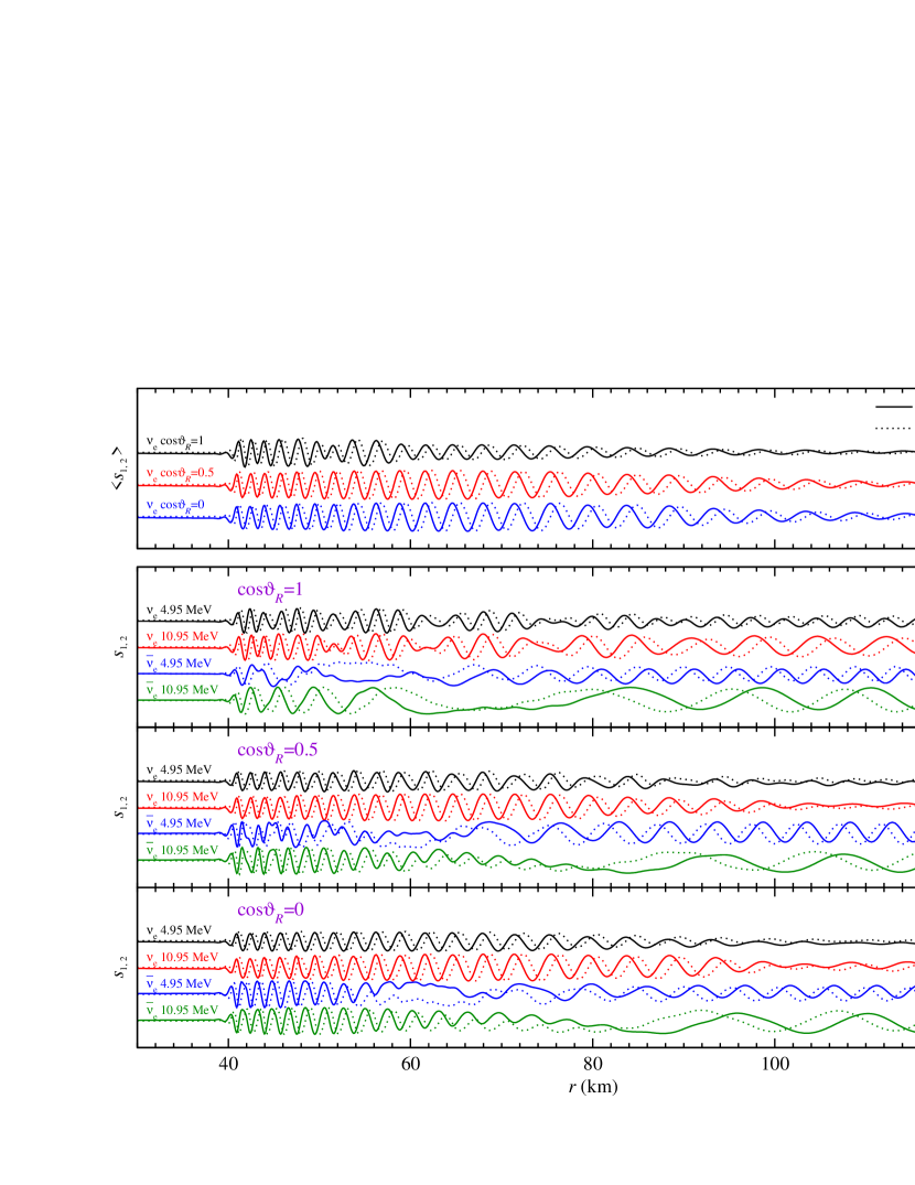
Figure 1: Oscillations of $s_{1}(r)$ (solid lines) and $s_{2}(r)$ (dotted lines), the projection of the NFIS on $\vec{e}_{1}$ and $\vec{e}_{2}$, respectively, as functions of $r$. The curves in the top panel are for neutrinos emitted as $\nu_{e}$ and propagating along trajectories with $\cos\vartheta_{R}=1$, $0.5$ and $0$, respectively. Here $\langle s_{1(2)}\rangle$ represents an average over the initial $\nu_{e}$ energy spectrum. Clearly $\langle\vec{s}(r)\rangle$ for various neutrino trajectories precesses about $\vec{e}_{3}$ in phase along $r$. The curves in the bottom panels show $s_{1,2}$ for individual energy and angle bins (as labelled). The neutrinos or antineutrinos corresponding to these curves start as pure $\nu_{e}$ or $\bar{\nu}_{e}$, as labelled. Note that $s_{1}(r)$ and $s_{2}(r)$ are phase-locked at low to modest radii and again at larger radii. This suggests that the NFIS’s for both neutrinos and antineutrinos precess with a common frequency at low to modest radii but precess with energy-dependent vacuum oscillation frequencies at larger radii. In addition, at large radii, the NFIS’s for antineutrinos precess in the opposite direction with respect to those for neutrinos.

In figure 1(a) we plot $\langle s_{1(2)}(r)\rangle$, the energy-averaged NFIS component, where $s_{1(2)}(r)\equiv\vec{s}_{p}(r)\cdot\vec{e}_{1(2)}$, as a function of $r$ for neutrinos emitted as pure $\nu_{e}$ and propagating along a few representative trajectories. We here do not distinguish between the vacuum mass basis and the flavour basis because $\theta_{\mathrm{v}}\ll 1$. Because of the spherical symmetry, it suffices to label different neutrino trajectories by neutrino emission angle $\vartheta_{R}$, which can be defined to be

$$\cos\vartheta_{r}(\hat{\bi{p}})\equiv\hat{\bi{p}}\cdot\hat{\bi{r}}$$ (94)

evaluated at $r=R$, with $\hat{\bi{r}}$ being the radial direction. (Note that we use $\theta$ and $\vartheta$ to denote angles in flavour space and coordinate space, respectively.) Figure 1(a) indeed shows that, as neutrino oscillations start at $r\simeq 40$ km, $\langle\vec{s}(r)\rangle$ begin to precess in phase about $\vec{e}_{3}$ along $r$. This is a clear signature of the existence of the collective precession mode in our numerical result.

In figures 1(b–d) we plot $s_{1,2}(r)$ for a dozen individual angular and energy bins for both neutrinos and antineutrinos. We observe that $s_{1}(r)$ and $s_{2}(r)$ for most neutrinos and antineutrinos are phase-locked at low to modest radii and again at larger radii. The phase-lock at the low to modest radii occurs because the neutrinos and antineutrinos participate in the collective precession mode, and the phase-lock at larger radii occurs because they experience vacuum oscillations. We note that the precession of NFIS’s in vacuum oscillations is energy dependent, and can be in the opposite direction to the sense of precession in the collective precession mode. This behaviour is especially prominent for the antineutrino modes in figure 1(d).

Two important trends in the breakdown of the collective precession mode merit further elaboration. One of these trends is that along each neutrino trajectory antineutrinos always drop out of the collective mode earlier than neutrinos, and antineutrinos with smaller energies drop out earlier than those with larger energies. This trend can be explained using the criterion in (87). Using (79) and the spherical symmetry of the supernova model we obtain

$$K(r)\equiv|\bi{K}(r)|=\lambda(r)C(r)-\langle\omega(r)\rangle,$$ (95)

where

$$C(r)\equiv\frac{\sum_{p}n_{p}(r)\tilde{P}_{p,1}(r)}{\sum_{p}\cos\vartheta_{r}(\hat{\bi{p}})\,n_{p}(r)\tilde{P}_{p,1}(r)}>1,$$ (96)

and

$$\langle\omega(r)\rangle\equiv\frac{\sum_{p}\omega_{p^{0}}n_{p}(r)\tilde{P}_{p,1}(r)}{\sum_{p}\cos\vartheta_{r}(\hat{\bi{p}})\,n_{p}(r)\tilde{P}_{p,1}(r)}.$$ (97)

Combining (85) and (95) we have

$$|\tilde{\mathsf{H}}^{\mathrm{ext}}_{p}(r)| =|\lambda(r)[C(r)\cos\vartheta_{r}-1]-[\langle\omega(r)\rangle\cos\vartheta_{r}-\omega_{p^{0}}]|,$$ (98)

$$\simeq|\omega_{p^{0}}-\langle\omega(r)\rangle|\qquad\textrm{if }r\gg R.$$ (99)

Note that in the inverted neutrino mass hierarchy case considered here, we have $\omega_{p^{0}}=\Delta m^{2}/(2p^{0})<0$ for neutrinos ($p^{0}>0$) and $\omega_{p^{0}}>0$ for antineutrinos ($p^{0}<0$). Because there are more neutrinos than antineutrinos, we expect $\langle\omega(r)\rangle<0$ in this calculation. From (99) one sees that $|\tilde{\mathsf{H}}^{\mathrm{ext}}_{p}(r)|$ is generally larger for antineutrinos, and the smaller the energy of the antineutrino is, the larger $|\tilde{\mathsf{H}}^{\mathrm{ext}}_{p}(r)|$ is. Therefore, along the same neutrino trajectory (and with the same value of $|\tilde{\mathsf{H}}^{\nu\nu}_{\vartheta_{R}}(r)|$), (87) is satisfied at lower radii for the antineutrinos with smaller energies. These antineutrinos must drop out of the collective precession mode earlier than other neutrinos do.

The second trend is that neutrinos and antineutrinos propagating along the radial trajectory ($\cos\vartheta_{R}=1$) drop out of the collective precession mode earlier than those with the same energies but propagating along the tangential trajectory ($\cos\vartheta_{R}=0$). This can also be explained using criterion (87). As a crude estimate of the strength of the neutrino self-interaction we can assume that NFIS’s are aligned or antialigned with each other and, therefore,

$$|\tilde{\mathsf{H}}^{\nu\nu}_{\vartheta_{R}}(r)| \propto 1-\sqrt{1-\left(\frac{R}{r}\right)^{2}}-\frac{1}{2}\left(\frac{R}{r}\right)^{2}\cos\vartheta_{r},$$ (100)

$$\simeq\frac{1}{2}\left(\frac{R}{r}\right)^{2}(1-\cos\vartheta_{r})+\frac{1}{8}\left(\frac{R}{r}\right)^{4}\quad\textrm{if }\left(\frac{R}{r}\right)^{2}\ll 1.$$ (101)

Clearly $|\tilde{\mathsf{H}}^{\nu\nu}_{\vartheta_{R}}(r)|$ is the weakest along the radial trajectory ($\cos\vartheta_{r}=\cos\vartheta_{R}=1$) for which (87) is satisfied first for a given neutrino energy.

4.2 Stepwise spectral swapping

In figure 2 we plot survival probabilities $P_{\nu\nu}(E,\vartheta_{R})$ at $r=200$ km as functions of both neutrino energy $E$ and emission angle $\vartheta_{R}$ for both neutrinos and antineutrinos. As in previous calculations, figure 2 shows that $\nu_{e}$ and $\nu_{x}$ swap their energy spectra at energies above $\sim 8$ MeV, a phenomenon termed as “stepwise spectral swapping” or “spectral split”.

$\begin{array}[]{@{}c@{\hspace{0.02 \textwidth}}c@{}}\includegraphics*[scale={0.38},keepaspectratio]{fig2a.eps}\hfil\hskip 8.67424pt&\includegraphics*[scale={0.38},keepaspectratio]{fig2b.eps}\end{array}$

Figure 2: The neutrino survival probabilities $P_{\nu\nu}(E,\vartheta_{R})$ as functions of neutrino energy $E$ and emission angle $\vartheta_{R}$ at $r=200$ km. The left panel is for neutrinos and the right panel is for antineutrinos. Shading code for $P_{\nu\nu}(E,\vartheta_{R})$ is given at right.

For the single-angle approximated supernova model or for homogeneous, isotropic neutrino gases the stepwise-spectral-swapping phenomenon can be explained as the result of the collective precession mode [18, 23, 20]. If all neutrinos in a homogeneous, isotropic neutrino gas remain in the collective precession mode to the very end, then the polarization vector becomes

$$\vec{P}_{p^{0}}=\epsilon_{p^{0}}\,\mathrm{sgn}(\omega_{\mathrm{pr}}^{0}-\omega_{p^{0}})\,\vec{e}_{3},$$ (102)

where $\epsilon=+1$ ($-1$) if $\vec{P}_{p^{0}}(t)$ is aligned (antialigned) with $\vec{\tilde{H}}_{p^{0}}(t)$, and $\omega_{\mathrm{pr}}^{0}$ is the common angular precession velocity of $\vec{P}_{p^{0}}(t)$ about $\vec{e}_{3}$ when $n_{\nu}^{\mathrm{tot}}\rightarrow 0$. As a result, the neutrino survival probability becomes

$$P_{\nu\nu}(E)\simeq\left\{\begin{array}[]{ll}1&\textrm{ for neutrinos with }E<E^{\mathrm{s}},\\ 0&\textrm{ for neutrinos with }E>E^{\mathrm{s}},\\ 0&\textrm{ for antineutrinos},\end{array}\right.$$ (103)

where

$$E^{\mathrm{s}}=\left|\frac{\Delta m^{2}}{2\omega_{\mathrm{pr}}^{0}}\right|.$$ (104)

The stepwise-spectral-swapping phenomenon in an anisotropic environment, such as shown in figure 2, can be understood through the collective precession mode discussed in section 3.4 in a way similar to above argument based on (102)–(104), except for the replacement $\omega_{\mathrm{pr}}^{0}\rightarrow-K|_{r\rightarrow\infty}$. In reality, however, neutrinos and antineutrinos are not indefinitely entrained in the collective precession mode. The breakdown in collective behaviour results in some interesting features as shown in figure 2. For example, as explained in section 4.1, antineutrinos, especially those with low energies and/or propagating along the radial trajectory, do not participate as well in the collective mode as other neutrinos do. Therefore, the simplistic prescription in equation (103) works better for neutrinos than for antineutrinos. In fact, according to figure 2, this prescription breaks down for antineutrinos with energies $\sim 5$ MeV and/or for those propagating along the radial trajectory. In addition, antineutrinos with energies $E\lesssim 0.8$ MeV do not participate in collective oscillations at all and are almost fully converted through the conventional matter-driven MSW mechanism. Antineutrinos with energies $E\sim 5$ MeV do participate in collective oscillations. However, they encounter MSW resonances after they leave the collective precession mode and, as a result, are (partially) converted back to their original flavours.

Another important detail in figure 2 is that the critical energy $E^{\mathrm{s}}$ is actually different for neutrinos propagating along different trajectories. In contrast, $K(r)$ is the same along these trajectories. Two main factors contribute to the variation of $E^{\mathrm{s}}$ from trajectory to trajectory. The first factor is that the collective precession frequency $K(r)\cos\vartheta_{r}$ along a neutrino world line depends on the neutrino propagation direction. It is largest along the radial trajectory and the smallest along the tangential trajectory. The second factor is that neutrinos propagating along different trajectories drop out of the collective precession mode at different radii. Neutrinos propagating along more radially-directed trajectories stop participating in collective oscillations at smaller distances from the proto-neutron star, but neutrinos propagating along more tangential trajectories stay in collective oscillations out to larger distances. Our numerical calculations show that the collective precession frequency always decreases as neutrino fluxes decrease. Therefore, both contributions lead to a smaller $E^{\mathrm{s}}$ for the radial trajectory and a larger $E^{\mathrm{s}}$ for the tangential trajectory. Indeed, the left panel of figure 2 shows that $E^{\mathrm{s}}$ for the radial and tangential trajectories differ by $\sim 0.7$ MeV.

5 Conclusions

We have demonstrated the existence of the SU($N_{\mathrm{f}}$) rotation symmetry in the neutrino flavour evolution equations. This symmetry can facilitate the establishment of the collective precession mode for neutrino flavour oscillations in various environments. The stepwise-spectral-swapping phenomenon can develop from such a collective neutrino oscillation mode in, e.g., supernovae. We have also given criteria for significant neutrino flavour oscillations to occur if neutrinos are entrained in the collective precession mode. These criteria can be used to understand the suppression of collective neutrino oscillations in anisotropic environments in the presence of a large matter density [28]. These criteria also illuminate the process of the breakdown of collective oscillations when neutrino densities are low. The results obtained in both our new simulation and previous multi-angle calculations for supernova neutrino oscillations can be understood in terms of the collective precession mode and the criteria we have provided.

There remains much to be learned about the collective precession mode for neutrino oscillations. This collective mode can not exist when there is no solution to (74) and (75). A related interesting observation is that collective oscillations, if any, for a symmetric system with equal numbers of neutrinos and antineutrinos are quickly disrupted in the presence of even an infinitesimal anisotropy and flavour equipartition is obtained as a result [26]. In the flavour pendulum analogy [36], the asymmetry of neutrinos and antineutrinos constitutes the internal spin of the flavour pendulum. The existence of this internal spin causes the flavour pendulum to undergo the precession which represents the collective precession mode for neutrino oscillations. There exists no collective precession mode in a symmetric neutrino system — this explains the finding in [26]. Meanwhile, it has been shown in [27] that a typical asymmetry in the neutrino and antineutrino fluxes in the supernova environment will suppress multi-angle decoherence and, therefore, make the collective precession mode for neutrino oscillations possible.

References

References

- [1] Fuller G M, Mayle R W, Wilson J R and Schramm D N 1987 Astrophys. J. 322 795
- [2] Nötzold D and Raffelt G 1988 Nucl. Phys. B 307 924
- [3] Pantaleone J T 1992 Phys. Rev. D 46 510
- [4] Samuel S 1993 Phys. Rev. D 48 1462
- [5] Kostelecký V A and Samuel S 1995 Phys. Rev. D 52 621 (Preprint arXiv:hep-ph/9506262)
- [6] Samuel S 1996 Phys. Rev. D 53 5382 (Preprint arXiv:hep-ph/9604341)
- [7] Pastor S, Raffelt G G and Semikoz D V 2002 Phys. Rev. D 65 053011 (Preprint arXiv:hep-ph/0109035)
- [8] Dolgov A D et al. 2002 Nucl. Phys. B 632 363 (Preprint arXiv:hep-ph/0201287)
- [9] Abazajian K N, Beacom J F and Bell N F 2002 Phys. Rev. D 66 013008 (Preprint arXiv:astro-ph/0203442)
- [10] Qian Y Z and Fuller G M 1995 Phys. Rev. D 51 1479 (Preprint arXiv:astro-ph/9406073)
- [11] Pastor S and Raffelt G 2002 Phys. Rev. Lett. 89 191101 (Preprint arXiv:astro-ph/0207281)
- [12] Balantekin A B and Yüksel H 2005 New J. Phys. 7 51 (Preprint arXiv:astro-ph/0411159)
- [13] Fuller G M and Qian Y Z 2006 Phys. Rev. D 73 023004 (Preprint arXiv:astro-ph/0505240)
- [14] Wolfenstein L 1978 Phys. Rev. D 17 2369
- [15] Mikheyev S P and Smirnov A Y 1985 Yad. Fiz. 42 1441 [Sov. J. Nucl. Phys. 42 913]
- [16] Duan H, Fuller G M and Qian Y Z 2006 Phys. Rev. D 74 123004 (Preprint arXiv:astro-ph/0511275)
- [17] Duan H, Fuller G M, Carlson J and Qian Y Z 2006 Phys. Rev. Lett. 97 241101 (Preprint arXiv:astro-ph/0608050)
- [18] Duan H, Fuller G M, Carlson J and Qian Y Z 2006 Phys. Rev. D 74 105014 (Preprint arXiv:astro-ph/0606616)
- [19] Duan H and Kneller J P 2009 Preprint arXiv:0904.0974
- [20] Raffelt G G and Smirnov A Y 2007 Phys. Rev. D 76 081301(R) (Preprint arxiv:0705.1830)
- [21] Duan H, Fuller G M and Qian Y Z 2007 Phys. Rev. D 76 085013 (Preprint arxiv:0706.4293)
- [22] Dasgupta B, Dighe A, Mirizzi A and Raffelt G G 2008 Phys. Rev. D 78 033014 (Preprint arXiv:0805.3300)
- [23] Duan H, Fuller G M, Carlson J and Qian Y Z 2007 Phys. Rev. D 75 125005 (Preprint arXiv:astro-ph/0703776)
- [24] Duan H, Fuller G M, Carlson J and Qian Y Z 2007 Phys. Rev. Lett. 99 241802 (Preprint arxiv:0707.0290)
- [25] Fogli G L, Lisi E, Marrone A and Mirizzi A 2007 JCAP 0712 010 (Preprint arxiv:0707.1998)
- [26] Raffelt G G and Sigl G G R 2007 Phys. Rev. D 75 083002 (Preprint arXiv:hep-ph/0701182)
- [27] Esteban-Pretel A, Pastor S, Tomas R, Raffelt G G and Sigl G 2007 Phys. Rev. D 76 125018 (Preprint arxiv:0706.2498)
- [28] Esteban-Pretel A et al. 2008 Phys. Rev. D 78 085012 (Preprint arXiv:0807.0659)
- [29] Sigl G and Raffelt G 1993 Nucl. Phys. B 406 423
- [30] Strack P and Burrows A 2005 Phys. Rev. D 71 093004 (Preprint arXiv:hep-ph/0504035)
- [31] Cardall C Y 2008 Phys. Rev. D 78 085017 (Preprint arXiv:0712.1188)
- [32] Gava J and Volpe C 2008 Phys. Rev. D 78 083007 (Preprint arXiv:0807.3418)
- [33] Dasgupta B and Dighe A 2008 Phys. Rev. D 77 113002 (Preprint arXiv:0712.3798)
- [34] Kim C W, Kim J and Sze W K 1988 Phys. Rev. D 37 1072
- [35] Raffelt G G 2008 Phys. Rev. D 78 125015 (Preprint arXiv:0810.1407)
- [36] Hannestad S, Raffelt G G, Sigl G and Wong Y Y Y 2006 Phys. Rev. D 74 105010 (Preprint arXiv:astro-ph/0608695)
- [37] Duan H, Fuller G M and Qian Y Z 2008 Phys. Rev. D 77 085016 (Preprint arXiv:0801.1363)
- [38] Dasgupta B, Dighe A, Mirizzi A and Raffelt G G 2008 Phys. Rev. D 77 113007 (Preprint arXiv:0801.1660)
- [39] Dighe A S and Smirnov A Y 2000 Phys. Rev. D 62 033007 (Preprint arXiv:hep-ph/9907423)
- [40] Schirato R C and Fuller G M 2002 Preprint arXiv:astro-ph/0205390
- [41] Kneller J P, McLaughlin G C and Brockman J 2008 Phys. Rev. D 77 045023 (Preprint arxiv:0705.3835)
- [42] Amsler C et al. (Particle Data Group) 2008 Phys. Lett. B 667 1