Coulomb corrections in quasi-elastic scattering: tests of the effective-momentum approximation

Abstract

Coulomb corrections for quasi-elastic scattering of electrons by nuclei are calculated using eikonal distorted waves. Corrections to the lowest-order eikonal approximation are included in order to obtain accurate results. Spin-dependent eikonal phase shifts are evaluated and they yield very small corrections to the longitudinal and transverse cross sections at electron energies of 500 MeV or higher. Because of this the Rosenbluth procedure is accurate for separation of the longitudinal and transverse response functions. The effective-momentum approximation is also found to be accurate with regard to removal of the remaining Coulomb effects from the distorted waves. Calculations are presented for electron scattering from ${}^{208}Pb$ and ${}^{56}Fe$ nuclei at energies of 500 MeV and 800 MeV and momentum transfers $q$ = 550 MeV/c and 900 MeV/c.

I Introduction

Measurements of cross sections for quasi-elastic electron scattering provide basic tests of our understanding of nuclei. Experiments have been performed at the MIT Bates Laboratory  Altemus83 ; Deady83 ; Hotta84 ; Deady86 ; Blatchley86 ; Dytman88 ; Dow88 ; Yates93 ; Williamson97 , at the Saclay Laboratory Barreau83 ; Meziani84 ; Meziani85 ; Marchand85 ; Zghiche94 ; Gueye99 and at SLAC Baran88 ; Chen91 ; Meziani92 in order to explore this reaction. A recent review of quasi-elastic scattering provides a guide to the experimental and theoretical results Benhar08 . Generally it is assumed that the reaction is dominated by the exchange of one hard photon between the electron and a nucleon in the nucleus. Many soft photons also are exchanged and their effects are described by distorted waves based on the Coulomb potential in the initial and final states of the electron. An important issue is to account for the effects of the Coulomb interaction in a manner that allows extraction of the nuclear response functions, $R_{L}$ and $R_{T}$, which correspond to plane-wave matrix elements of the longitudinal and transverse parts of the currents. After the nucleon form factor is divided out, the longitudinal response function at a fixed and sufficiently large value of the momentum transfer, q, is expected to satisfy a Coulomb sum rule, i.e., $\int d\omega S_{L}(q,\omega)\approx Z$, where Z is the number of protons. Such a sum rule should hold under general conditions for a nonrelativistic description of nuclear wave functions and currents provided only that $q$ is sufficiently large to make the effects of correlations small. Although the response functions are affected by the final-state interactions (FSI), the sum rule should not be affected by them because it relies on a sum over a complete set of final states of the nucleus. When relativistic effects in the nuclear current are taken into account, there are minor relativistic corrections to the sum rule but it remains useful. However, attempts to verify it experimentally have produced puzzling results and controversy about Coulomb corrections.

In order to obtain the longitudinal response function, it is conventional to perform a Rosenbluth separation after dividing the cross section by the Mott cross section $\sigma_{M}$ and some kinematical factors,

$$\frac{1}{\sigma_{M}}\frac{d\sigma}{d\Omega d\omega}~{}\epsilon~{}\frac{q^{4}}{Q^{4}}=\epsilon~{}R_{L}^{expt}(q,\omega)+\frac{1}{2}\Biggr{(}\frac{q^{2}}{Q^{2}}\Biggr{)}~{}\ R_{T}^{expt}(q,\omega)$$ (1)

with $Q^{2}=\omega^{2}-q^{2}$ and where $\sigma_{M}=4\alpha^{2}E_{f}^{2}cos^{2}(\frac{1}{2}\theta_{e})/Q^{4}$. The longitudinal virtual-photon polarization is defined as

$$\epsilon=\Biggr{(}1+\frac{2q^{2}}{Q^{2}}tan^{2}\frac{\theta_{e}}{2}\Biggr{)}^{-1}.$$ (2)

At fixed $q$ and $\omega$, it varies from 0 to 1 as the electron scattering angle $\theta_{e}$ varies from 180 to 0 degrees. Measurements of the cross section at different values of $\epsilon$ for fixed values of $q$ and $\omega$ allow a separation of the experimental response functions, $R_{L}^{expt}$ and $R_{T}^{expt}$. The $R_{L}^{expt}$ that is extracted from experimental cross section as in Eq. (1) can differ from the desired $R_{L}$, which is the plane-wave matrix element of the longitudinal current, for two reasons. One is that Coulomb corrections associated with spin-dependent effects in the electron wave functions can cause the contributions of the longitudinal and transverse currents to have different dependence on $\theta_{e}$ than is assumed in the Rosenbluth separation. Co87 The other is that Coulomb distorted waves alter the response. These Coulomb corrections should be removed before the Coulomb sum rule can be evaluated. In addition, nucleon form factors should be divided out of the longitudinal response function. A standard approach to modeling the Coulomb corrections is to use the distorted wave Born approximation (DWBA). One solves the Dirac equation for the electron distorted waves in the presence of the Coulomb potential for both the initial and final states of the electron. Jin9294 ; Udias93 ; Udias95 ; Kim01 When these distorted waves are combined with nuclear wave functions obtained from a model of nuclear structure, and appropriate current operators, cross sections may be calculated and compared with experimental results. The DWBA analysis involves extensive numerical calculations. Owing to the infinite range of the Coulomb potential, partial-wave expansions converge very slowly, the more so as the energy increases.

A number of works have used the eikonal approximation in order to simplify the analysis at high energies. The use of the eikonal approximation also must be accompanied by inclusion of ”focusing factors” that are not present in the eikonal wave functions. Yennie65 ; Lenz71 ; Rosenfelder80 Czyz and Gottfried Czyz63 used the eikonal approximation to analyze electron scattering but that work did not include focusing factors. An analysis based on the Schrodinger equation showed that the corrections to the eikonal approximation generally produce a focusing factor in the wave function. Baker72 Work by Giusti et al. also is based on the eikonal approximation Giusti87 ; Giusti88 and some recents works have combined the eikonal approximation with semi-classical focusing factors in order to assess Coulomb corrections in quasi-elastic scattering. Aste04a ; Aste04b

A very simple effective-momentum approximation (EMA) for treating the Coulomb corrections was developed by RosenfelderRosenfelder80 and Triani et al. Traini01 ; Traini88 . In the EMA the effects of the Coulomb potential are incorporated as shifts of the initial and final electron momentum values that should be used in a plane-wave Born approximation (PWIA) analysis. The shifted electron momenta are the effective momenta. They imply a corresponding shift of the photon momentum, $q\rightarrow q_{eff}$.

Interpretations of quasi-elastic data depend upon many experimental details and different experiments have produced significantly different values of the Coulomb sum rule. Morgenstern01 ; Benhar08 In addition to possible experimental differences, there are theoretical differences in the analysis of the Coulomb corrections because the DWBA analysis based on partial waves has been used for some experiments and the EMA analysis has been used for others. Sometimes it is assumed that the nucleon form factors can be pulled out of the matrix element and evaluated at the momentum transfer of the electron. Kim01 At other times the form factors are evaluated at the effective photon momentum, $q_{eff}$.

In order to address questions about the theoretical differences in the treatment of Coulomb distorted waves, we developed a systematic eikonal expansion in Ref. Tjon&Wallace06 that provides more accurate eikonal wave functions for a DWBA analysis. The accuracy is good enough to eliminate concerns about use of the eikonal approximation at the energies of interest. Moreover the ”focusing factors” arise naturally as part of the corrections to the eikonal approximation and the ad-hoc procedure of incorporating them is replaced by a systematic procedure. The eikonal expansion was found to converge rapidly at electron energies of interest. It has the advantage of providing insight into the nature of the Coulomb corrections because the focusing factors, the eikonal phase shifts that determine the momentum shifts and spin-dependent effects can be isolated for study.

In order to assess the accuracy of the EMA using the eikonal wave functions, we used in Ref. Tjon&Wallace06 a very simple model of the nuclear wave functions and we neglected the spin-dependent Coulomb corrections for simplicity. In order to compare full DWBA calculations of $R_{L}$ with the results based on the EMA, the DWBA results were fit to the EMA formula,

$$R_{L}({\bf q},\omega)=A~{}R_{L}^{PWIA}({\bf q}_{eff},\omega),$$ (3)

where the effective photon momentum is given by

$${\bf q}_{eff}=\hat{k}_{i}\Big{[}k_{i}-\delta k\Big{]}-\hat{k}_{f}\Big{[}k_{f}-\delta k\Big{]}.$$ (4)

There are two parameters in our EMA fits: the momentum-shift $\delta k$ and the overall normalization constant $A\approx 1$. Usually the parameter $A$ is assumed to be unity when experimental data are fit using Eq. (3). In model calculations that assumption can be checked because the PWIA response is known in the model. A factor $f_{EMA}$ can be used to relate $\delta k$ to the Coulomb potential at $r=0$, as follows,

$$f_{EMA}=\frac{\delta k}{V_{c}(0)}.$$ (5)

The factor $f_{EMA}$ is approximately the same for different nuclei. We found momentum shifts in Fig. 7 of Ref. Tjon&Wallace06 that correspond to $f_{EMA}(\omega)\approx 0.7$ near the peak of the response function for 500 MeV $e^{-}$ scatttering. Larger values of $f_{EMA}$ up to about 1 were found at the smallest and largest $\omega$ values but the response is small at those points. Although fits of the DWBA results can be made more precise by allowing $\delta k$ to depend on the energy loss, $\omega$, in this work we use a constant shift $\delta k$. That yields reasonable results and is simpler and thus preferable for the analysis of experimental data.

If the momentum-shift $\delta k$ and normalization constant $A$ are determined theoretically for a given nucleus such that the DWBA response is well described by the EMA fit of Eq. (3), then one may equate $R_{L}({\bf q},\omega)$ at fixed electron beam energy, $E$, and fixed momentum transfer ${\bf q}$ to a constant $A$ times the PWIA response function evaluated at the effective momentum transfer. That would remove the Coulomb effects to a reasonable approximation and allow the PWIA response to be extracted from experimental data. We expect similar Coulomb corrections for a variety of nuclear models. Aste08 The goal is to remove them with minimal reliance on any nuclear model. However, it must first be determined how well $R_{L}$ can be extracted from experimental data.

The spin-dependence of the eikonal wave functions was omitted in our previous paper, which left unanswered the question of the accuracy with which the desired response functions might be extracted from experimental cross sections. That is the first issue addressed in this paper. In Sec. II we restate the essential results of the eikonal expansion for Dirac wave functions and focus on the spin-dependent eikonal corrections. These are shown to provide very small differences to quasi-elastic cross sections, i.e., the helicity matrix elements of the electron current are very close to those based on the PWIA. The consequence is that when both initial and final electron energies are 200 MeV or more, the usual Rosenbluth separation provides an accurate separation of $R_{L}$ and $R_{T}$, well within the limits of experimental accuracy. Although the Rosenbluth separation should be accurate, there remain significant Coulomb effects within $R_{L}$. They can be treated with reasonable accuracy by use of the effective momentum approximation.

In order to determine more realistic values of the momentum shift, $\delta k$, shell model wave functions are used to describe the nucleus in this work. Our calculations are simplified by use of an approximation that is introduced by us in Ref. TjW08 and described in Section III, and which is denoted EMAr. That approximation applies the effective momentum approximation to the hard-photon propagator and form factors in order to reduce the numerical evaluation to a three-dimensional integration that provides a careful treatment of the full ${\bf r}$-dependence of the Coulombic effects from the electron wave functions. In the EMAr analysis, the nuclear current is handled in terms of a hadronic tensor, which can be extended to include the neutron contributions to cross sections. A comparison of the full DWBA and EMAr calculations for the 1s shell of ${}^{208}Pb$ shows close agreement of the results.

Section IV presents numerical calculations for quasi-elastic scattering by ${}^{208}Pb$ and ${}^{56}Fe$ using kinematics that are relevant to a recent experiment at Jefferson Laboratory. The nuclear model used is simple and a number of significant effects are omitted from the calculations, such as final-state interactions Horikawa80 , correlations, Benhar89 ; Sick07 and pion and $\Delta$ production vanOrden ; Dekker , but the calculated cross sections are expected to be roughly similar to experimental ones. The main goal is to determine suitable fitting parameters for use in applying Eq. (3) to experimental data so as to determine $R_{L}^{PWIA}$. Conclusions are presented in Section V.

II Quasi-elastic response functions

Because electron energies of interest generally are much greater than the electron mass, and the Coulomb potential and photon exchange are vector interactions, electron helicity is conserved to a very high degree of accuracy in quasi-elastic scattering. For example, using 500 MeV electrons one finds that the helicity is conserved except for terms of relative order $m_{e}^{2}/E^{2}\approx 10^{-6}$. In this work we keep only the effects that are consistent with helicity conservation.

The distorted-wave Born approximation is used with eikonal wave functions for the electron. For outgoing-wave (+) or incoming-wave (-) boundary conditions, the Dirac wave functions for potential $V(r)$ are written as Tjon&Wallace06

$$\Psi^{(\pm)}_{k,\lambda}({\bf r}) = \begin{pmatrix}u^{(\pm)}({\bf r})\cr 2\lambda u^{(\pm)}({\bf r})\end{pmatrix}\xi_{\lambda},$$

$$u^{(\pm)}({\bf r}) = \left(1-\frac{V}{E_{2}}\right)^{1/2}e^{ikz}e^{i\chi^{(\pm)}}e^{-\omega^{(\pm)}}e^{i\sigma_{e}\bar{\gamma}^{(\pm)}},$$ (6)

where $\xi_{\lambda}$ is a two-component helicity spinor and $\lambda=\pm\frac{1}{2}$ is the helicity eigenvalue. The lower components of the Dirac spinor are simply $2\lambda$ times the upper components because the electron mass is neglected. The wave propagates in the $z$-direction, which is along the asymptotic momentum ${\bf k}$, and an impact vector ${\bf b}$ is defined as the part of ${\bf r}$ that is perpendicular to the $\hat{z}$-direction. The eikonal phases $\chi^{(\pm)}$, $\omega^{(\pm)}$ and $\bar{\gamma}^{(\pm)}=\gamma^{(\pm)}\pm i\delta^{(\pm)}$ are obtained from integrals over the potential along the z-direction as shown in Ref. Tjon&Wallace06 . The spin matrix in the eikonal phase is $\sigma_{e}=\sigma\cdot\hat{b}\times\hat{z}$, the energy is $E$ and $E_{2}=E+m$.

II.1 DWBA analysis

The DWBA cross section for knockout of a nucleon of momentum ${\bf p}$ involves a two-dimensional integration over the angles of the knocked-out nucleon as follows,

$$\frac{1}{\sigma_{M}}\frac{d\sigma}{d\Omega d\omega}=\frac{Q^{4}}{cos^{2}(\frac{\theta_{e}}{2})}\sum_{nlm}\int d\Omega_{p}\frac{pE_{p}}{(2\pi)^{5}}\bigr{|}{\cal M}_{nlm}\bigr{|}^{2}.$$ (7)

Omitting the final-state interactions of the nucleon, the matrix element for quasi-elastic knockout involves a six-dimensional integration,

$${\cal M}_{nlm} = \frac{1}{(2\pi)^{2}}\int d^{3}q^{\prime}\int d^{3}r\overline{\Psi}_{k_{f},\lambda_{f}}^{(-)*}({\bf r})\gamma^{\mu}e^{-i{\bf q^{\prime}}\cdot{\bf r}}\Psi_{k_{i},\lambda_{i}}^{(+)}({\bf r})\frac{j_{N\mu}({\bf q^{\prime}},{\bf p})}{{\bf q^{\prime}}^{2}-\omega^{2}}\psi_{nlm}({\bf q^{\prime}}-{\bf p})$$ (8)

$$= \frac{1}{(2\pi)^{2}}\int d^{3}q^{\prime}\int d^{3}re^{i({\bf q}-{\bf q^{\prime}})\cdot{\bf r}}h_{e}^{\mu}({\bf r})f_{f}f_{i}e^{i\chi}\frac{j_{N\mu}({\bf q^{\prime}},{\bf p})}{{\bf q^{\prime}}^{2}-\omega^{2}}\psi_{nlm}({\bf q^{\prime}}-{\bf p})$$

where $j_{N\mu}({\bf q^{\prime}},{\bf p})$ is the nucleon current, $h_{e}^{\mu}$ is a four-vector of helicity matrix elements of the electron current and $\psi_{nlm}({\bf q^{\prime}}-{\bf p})$ is the momentum-space wave function of a nucleon in the nucleus with quantum numbers n (radial), l (angular momentum) and m (z-component of angular momentum). Subscripts $i$ and $f$ refer to the initial and final electron states with asymptotic momenta ${\bf k}_{i}$ and ${\bf k}_{f}$ that provide the respective z-directions for incoming and outgoing waves. The exchanged photon has energy $\omega$ and momentum ${\bf q^{\prime}}$, the initial electron helicity is $\lambda_{i}$ and the final electron helicity is $\lambda_{f}$. The momentum transferred by the electron is ${\bf q}={\bf k}_{i}-{\bf k}_{f}$ and it differs from the momentum ${\bf q^{\prime}}$ of the photon because of the Coulomb effects. Nucleon form factors within the nucleon current depend on the photon momentum, $q^{\prime}$, that is integrated. The sum of eikonal phases for incoming and outgoing waves is $\chi=\chi_{f}^{(-)}({\bf r})+\chi_{i}^{(+)}({\bf r})$ and the focusing factors are defined by

$$f_{i}({\bf r}) = \Biggr{(}1-\frac{V}{E_{2i}}\Biggr{)}^{1/2}e^{-\omega_{i}^{(+)}},$$

$$f_{f}({\bf r}) = \Biggr{(}1-\frac{V}{E_{2f}}\Biggr{)}^{1/2}e^{-\omega_{f}^{(-)}},$$ (9)

where $E_{2i}=E_{i}+m$ and $E_{2f}=E_{f}+m$.

The Coulomb potential for scattering from a ${}^{208}Pb$ nucleus is shown in Fig. 1. The solid line shows the potential based on a fit of experimental data for the charge density de_Vries87 and the dash line shows the simple potential used in our calculations, namely,

$$V_{c}(r)=\frac{-V_{0}}{(r^{2}+R^{2})^{1/2}}.$$ (10)

The simple potential allows an analytical evaluation of the eikonal phases. The parameters $V_{0}$ and $R$ are chosen so that the simple potential has the same value as the empirical potential at $r=0$ and the same average value as the potential based on experimental data in the sense that $\int dr\rho_{expt}(r)V_{c}(r)=\int dr\rho_{expt}(r)V_{expt}(r)$. This ensures that $V_{c}(r)$ provides a good fit in the range where the nuclear density is significant (the dot-dash line shows one-tenth the nuclear charge density for reference).

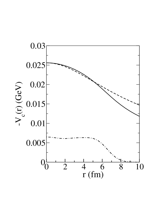
Figure 1: Coulomb potential for ${}^{208}Pb$. The solid line shows the potential based on the empirically determined charge density. de_Vries87 The dash line shows the approximate potential used in this work based on parameter values $V_{0}$ = 0.0256 GeV and $R=$7.1 fm. The dash-dot line shows one-tenth the charge density, $0.1\rho_{ch}(r)$, for ${}^{208}Pb$.

Eikonal phases based on the Coulomb potential of Eq. (10) are shown in Fig. 2. The phases $\chi_{i}^{(+)}$ and $\omega_{i}^{(+)}$ are shown as a function of impact parameter $|{\bf b}|$ at $z=0$ and the nucleus is located at ${\bf b}=0$, $z=0$. Note that $\chi_{i}^{(+)}$ and $\chi_{f}^{(-)}$ each have the same behavior at $z=0$ and the total phase $\chi=\chi_{i}^{(+)}+\chi_{f}^{(-)}$ is approximately double the values shown. Figure 2 shows that the eikonal expansion produces well converged results for the wave function at electron energy equal to 500 MeV for scattering from ${}^{208}Pb$.

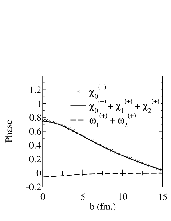
Figure 2: Eikonal phases at $z=0$ for 500 MeV electron scattering from ${}^{208}Pb$.

Coulomb corrections affect the helicity matrix elements of the electron current because of the spin-dependent eikonal phases involving $\bar{\gamma}^{(\pm)}$ as follows,

$$h_{e}^{\mu}({\bf r})=\delta_{\lambda_{f}\lambda_{i}}\xi^{{\dagger}}_{\lambda_{f}}(\theta_{e})e^{i\sigma_{e_{f}}\bar{\gamma}_{f}^{(-)*}}\Big{\{}1,2\lambda_{i}\vec{\sigma}\Big{\}}e^{i\sigma_{e_{i}}\bar{\gamma}_{i}^{(+)}}\xi_{\lambda_{i}}.$$ (11)

As shown in Tjon&Wallace06 , the required helicity matrix elements are given by

$$h_{e}^{0} = A_{2\lambda_{i}}cos{1\over 2}\theta_{e}+C_{2\lambda_{i}}sin{1\over 2}\theta_{e}\longrightarrow cos{1\over 2}\theta_{e},$$

$$h_{e}^{x} = B_{2\lambda_{i}}sin{1\over 2}\theta_{e}+D_{2\lambda_{i}}cos{1\over 2}\theta_{e}\longrightarrow sin{1\over 2}\theta_{e},$$

$$h_{e}^{y} = 2i\lambda_{i}\Bigr{(}A_{2\lambda_{i}}sin{1\over 2}\theta_{e}-C_{2\lambda_{i}}cos{1\over 2}\theta_{e}\Bigr{)}\longrightarrow 2i\lambda_{i}sin{1\over 2}\theta_{e},$$

$$h_{e}^{z} = B_{2\lambda_{i}}cos{1\over 2}\theta_{e}-D_{2\lambda_{i}}sin{1\over 2}\theta_{e}\longrightarrow cos{1\over 2}\theta_{e}.$$

The Rosenbluth separation implicitly assumes that the helicity matrix elements take the plane-wave values that are shown following the arrows in Eq. (LABEL:eq:helicityfacs). One sees in Eq. (LABEL:eq:helicityfacs) that the spin-dependent Coulomb effects cause each component of the four-vector of electron helicity matrix elements to involve both $cos{1\over 2}\theta_{e}$ and $sin{1\over 2}\theta_{e}$. This property carries over to the longitudinal and transverse currents. Consequently, $R_{L}^{expt}$ and $R_{T}^{expt}$ extracted using the Rosenbluth separation each involve admixtures of the longitudinal and transverse currents.

The spin-orbit parts of the eikonal phases enter the helicity matrix elements in the following four combinations as shown in Ref. Tjon&Wallace06 ,

$$A_{2\lambda_{i}}\equiv cos\bar{\gamma}_{f}^{(-)*}cos\bar{\gamma}_{i}^{(+)}-sin\bar{\gamma}_{i}^{(+)}sin\bar{\gamma}_{f}^{(-)*}e^{2i\lambda_{i}(\phi_{i}-\phi_{f})},$$

$$B_{2\lambda_{i}}\equiv cos\bar{\gamma}_{f}^{(-)*}cos\bar{\gamma}_{i}^{(+)}+sin\bar{\gamma}_{i}^{(+)}sin\bar{\gamma}_{f}^{(-)*}e^{2i\lambda_{i}(\phi_{i}-\phi_{f})},$$

$$C_{2\lambda_{i}}\equiv cos\bar{\gamma}_{f}^{(-)*}sin\bar{\gamma}_{i}^{(+)}e^{2i\lambda_{i}\phi_{i}}+cos\bar{\gamma}_{i}^{(+)}sin\bar{\gamma}_{f}^{(-)*}e^{-2i\lambda_{i}\phi_{f}},$$

$$D_{2\lambda_{i}}\equiv cos\bar{\gamma}_{f}^{(-)*}sin\bar{\gamma}_{i}^{(+)}e^{2i\lambda_{i}\phi_{i}}-cos\bar{\gamma}_{i}^{(+)}sin\bar{\gamma}_{f}^{(-)*}e^{-2i\lambda_{i}\phi_{f}}.$$

(13)

Figure 3 shows the eikonal phases $\gamma^{(+)}$ and $\delta^{(+)}$ that are the real and imaginary parts of $\bar{\gamma}^{(+)}$. There is a simple relation between the phases as follows,

$$\bar{\gamma}^{(\pm)}({\bf r})=\gamma^{(\pm)}({\bf r})\pm i\delta^{(\pm)}({\bf r})=\frac{1}{2(E+m)}\frac{d}{db}\Big{(}\chi^{(\pm)}({\bf r})\pm i\omega^{(\pm)}({\bf r})\Big{)}.$$ (14)

This relation has been corrected from the one given in Ref. Tjon&Wallace06 because a factor $\frac{1}{2}$ was omitted there.

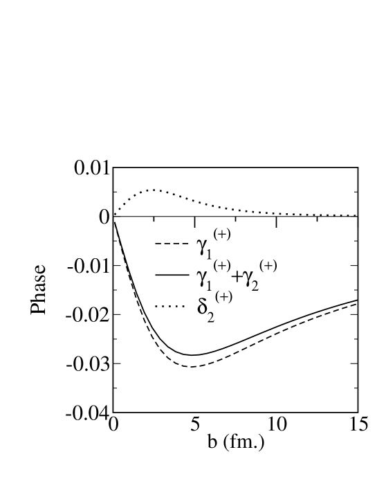
Figure 3: Spin phases for 500 MeV electron scattering from ${}^{208}Pb$.

Our previous numerical calculations omitted the spin-dependent Coulomb corrections, using instead the PWIA helicity matrix elements that are indicated following the arrows in Eq. (LABEL:eq:helicityfacs). In this work we include the spin-dependent Coulomb corrections and find the important result that they provide negligible corrections to quasi-elastic cross sections. This can be understood qualitatively as follows. For a 500 MeV electron scattering from the Coulomb potential of a ${}^{208}Pb$ nucleus, the phase $\bar{\gamma}^{(+)}=\gamma^{(+)}+i\delta^{(+)}$ typically has magnitude of 0.03 or less as shown in Fig. 3. It vanishes at zero impact parameter. Consequently, the coefficients $A_{2\lambda_{i}}\approx 1+{\cal O}(\bar{\gamma})^{2}$ and $B_{2\lambda_{i}}\approx 1+{\cal O}(\bar{\gamma})^{2}$ are very close to unity. The coefficients $C_{2\lambda_{i}}$ and $D_{2\lambda_{i}}$ have contributions that are first order in $\bar{\gamma}$. They also involve phase factors $e^{2i\lambda_{i}\phi_{i}}$ or $e^{2i\lambda_{i}\phi_{f}}$, where $tan\phi_{f}=tan\phi_{i}/\Big{(}cos\frac{\theta_{e}}{2}-sin\frac{\theta_{e}}{2}/(tan\theta_{i}cos\phi_{i})\Big{)}$ with $\theta_{i}$ and $\phi_{i}$ being the angles of the vector ${\bf r}$ relative to the polar axis along $\hat{k}_{i}$. When current matrix elements are integrated over ${\bf r}$ and summed over helicities, cancellations stemming from these phase factors cause the contributions to be very small. Current matrix elements are Fourier transforms and the $\phi_{i,f}$ dependent phase factors can receive support in the integration. However, the quasi-free cross sections involve an additional integration over angles of the knocked-out proton. The net effect is to reduce substantially the contributions from terms that involve the azimuthal angles $\phi_{i,f}$. Our numerical results show that cross sections calculated with the spin-dependent Coulomb corrections included are closer than one part per thousand to ones calculated using the PWIA helicity matrix elements. An example of this is shown in Figure 4, which shows the ratio of longitudinal response functions (calculated from Eq. (30)) with and without the spin-dependent Coulomb corrections at 500 MeV electron energy. Only for large energy loss, where the final state electron energy becomes small, does the ratio differ from unity by more that a few parts in ten thousand. For reference, the dotted line shows the variation of $1+.0001R_{L}$. Note that for energy loss $\omega$ = 300 MeV, the final electron energy is 200 MeV, but the ratio of cross sections with and without the Coulomb spin corrections differs from unity by less that one part per thousand. As the energy loss increases, the Coulomb spin corrections become relatively more important but the response function is decreasing to zero. The net effect is that the absolute error in the response function is about one part in ten thousand of the maximum value of $R_{L}$.

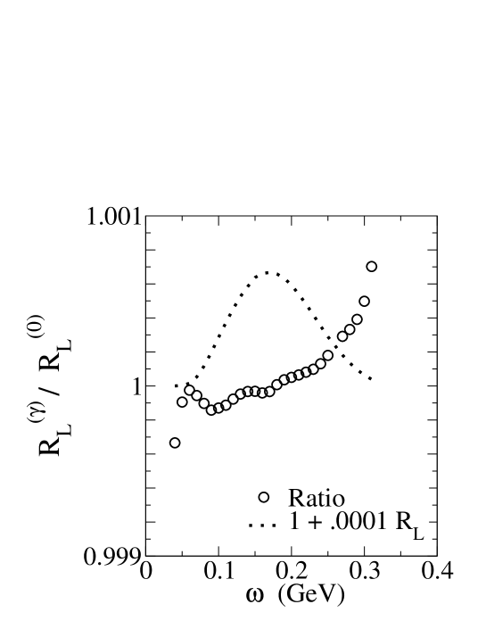
Figure 4: Circles show the ratio of the longitudinal response function $R_{L}^{(\gamma)}$ that includes the spin-dependent Coulomb corrections to the longitudinal response function $R_{L}^{(0)}$ that omits them for 500 MeV electron scattering from ${}^{208}Pb$ at q=550 MeV/c. The dotted line shows $1+.0001R_{L}$. Note that the effects of the spin-dependent Coulomb corrections are largest for $\omega$-values where the response function is a small fraction of its maximum value.

This is important because the helicity matrix elements govern the dependence of the cross sections on the electron scattering angle, $\theta_{e}$, at fixed $q$. When the PWIA helicity matrix elements provide an accurate approximation, the angle dependence is the same as in PWIA cross sections, and the Rosenbluth separation can be used to extract the longitudinal and transverse current matrix elements. We find negligible mixing of actual longitudinal and transverse current matrix elements in the response functions extracted using the Rosenbluth separation for all the cases evaluated in this paper.

Significant Coulombic effects remain in the $R_{L}$ and $R_{T}$ response functions that can be extracted by use of the Rosenbluth separation because of the spin-independent Coulomb effects. They may be treated using an effective momentum approximation.

III Effective photon momentum approximation

Because the effective-momentum approximation was found to be accurate in our prior work, in this work we approximate the photon momentum ${\bf q^{\prime}}$ that appears in the photon propagator and the nucleon current of Eq. (8) by an effective momentum ${\bf q}_{eff}$ as follows,

$$\frac{j_{\mu}^{N}({\bf p},{\bf q^{\prime}})}{{\bf q^{\prime}}^{2}-\omega^{2}} \rightarrow\frac{j_{\mu}^{N}({\bf p},{\bf q}_{eff})}{{\bf q}^{2}_{eff}-\omega^{2}},$$ (15)

where ${\bf q}_{eff}$ is given in Eq. (4). Note that this approximation also evaluates the nucleon form factors within the nucleon current at the effective photon momentum. This is a minimal use of the effective-momentum approximation designed to reduce the computation to a three-dimensional form, i.e., the approximation allows the photon propagator and the nuclear current to be factored out of the integral over ${\bf q^{\prime}}$, which is then performed to obtain $\int\frac{d^{3}q^{\prime}}{(2\pi)^{3}}e^{-i{\bf q^{\prime}}\cdot{\bf r}}\psi_{nlm}({\bf q^{\prime}}-{\bf p})=e^{-i{\bf p}\cdot{\bf r}}\psi_{nlm}({\bf r})$. This yields

$${\cal M}_{nlm}\longrightarrow{\cal M}^{EMAr}_{nlm}=\frac{2\pi}{Q^{2}_{eff}}j_{\mu}^{N}({\bf p},{\bf q}_{eff})\,{\cal M}^{\mu}_{nlm}$$ (16)

where $Q^{2}_{eff}={\bf q}^{2}_{eff}-\omega^{2}$ and we define

$${\cal M}^{\mu}_{nlm}=\int d^{3}re^{i({\bf Q}-{\bf p})\cdot{\bf r}}e^{i\chi({\bf r})}\,f_{i}({\bf r})f_{f}({\bf r})\,h_{e}^{\mu}({\bf r})\,\psi_{nlm}({\bf r}).$$ (17)

This procedure has been discussed in Ref TjW08 and is called the EMAr approximation. It has the advantage over the usual EMA of not approximating the r-dependence of the eikonal phases and focusing factors that provide the Coulomb corrections to the electron wave functions. The three-dimensional integration of Eq. (17) provides a good correspondence with the full DWBA analysis at much lower computational cost. Procedures to determine appropriate values of $\delta k$, and thus the effective photon momentum that is factored out of the integral, are discussed further on.

III.1 Hadronic tensor

In the EMAr analysis, the bound-state nucleon’s wave function is taken to be a product of a Dirac spinor, $u({\bf p}-{\bf q})$, times a nonrelativistic wave function for a nucleon, i.e., $(M/(E_{{\bf p}-{\bf q}})^{1/2}u({\bf p}-{\bf q})\psi_{nlm}({\bf p}-{\bf q})$, and the knocked-out nucleon’s wave function is a Dirac spinor, $(M/E_{p})^{1/2}u({\bf p})$. The relevant nucleon current is

$$j^{N}_{\mu}=K^{1/2}\bar{u}({\bf p})\Big{[}\gamma_{\mu}F_{1}+\frac{i\kappa}{2M}F_{2}\sigma_{\mu\nu}q^{\nu}\Big{]}u({\bf p}-{\bf q}),$$ (18)

where $F_{1}(Q^{2})$ and $F_{2}(Q^{2})$ are nucleon form factors, $\kappa$ is the anomalous magnetic moment and $K=M^{2}/(E_{p}E_{{\bf p}-{\bf q}})$ is a normalization factor arising from the spinors. The EMAr cross section for knock-out of a nucleon of momentum ${\bf p}$ by absorption of a photon then takes the form

$$\frac{1}{\sigma_{M}}\frac{d\sigma}{d\Omega d\omega}=\frac{Q^{4}}{cos^{2}(\frac{\theta_{e}}{2})}\sum_{nlm}\int d\Omega_{p}\frac{4pE_{p}}{(2\pi)^{3}}\frac{K}{(q^{2}_{eff}-\omega^{2})^{2}}{\cal M}^{\mu}_{nlm}W_{\mu\nu}(p,q_{eff}){\cal M}^{\nu{\dagger}}_{nlm}$$ (19)

where the hadronic tensor is,

$$W_{\mu\nu}(p,q)=\frac{1}{2}Tr\Bigr{[}\frac{p\!\!\!/+M}{2M}\Bigr{(}\gamma_{\mu}F_{1}+i\frac{\kappa}{2M}F_{2}\sigma_{\mu\alpha}q^{\alpha}\Bigr{)}\frac{p\!\!\!/-q\!\!\!/+M}{2M}\Bigr{(}\gamma_{\nu}F_{1}+i\frac{\kappa}{2M}F_{2}\sigma_{\nu\beta}q^{\beta}\Bigr{)}\Bigr{]}.$$ (20)

Carrying out the trace over nucleon spins produces

$$W_{\mu\nu}(p,q)=\frac{1}{2}g_{\mu\nu}F_{1}^{2}+\frac{p_{\mu}(p-q)_{\nu}+(p-q)_{\mu}p_{\nu}-p\cdot(p-q)g_{\mu\nu}}{2M^{2}}F_{1}^{2}$$

$$+\Bigr{(}\frac{\kappa}{2M^{2}}F_{1}F_{2}+\frac{\kappa^{2}}{8M^{2}}F_{2}^{2}\Bigr{)}\Big{(}q^{2}g_{\mu\nu}-q_{\mu}q_{\nu}\Big{)}$$

$$+\frac{\kappa^{2}}{8M^{2}}F_{2}^{2}\Bigr{[}-q_{\mu}q_{\nu}\big{(}p^{2}+p\cdot q\big{)}+2\big{(}q_{\mu}p_{\nu}+p_{\mu}q_{\nu}\big{)}\big{(}q^{2}-p\cdot q\big{)}+\big{(}2p\cdot q-q^{2}\big{)}p\cdot qg_{\mu\nu}$$

$$-q^{2}\big{(}2p_{\mu}p_{\nu}-p^{2}g_{\mu\nu}\big{)}\Bigr{]}.$$ (21)

The hadronic tensor is gauge invariant when the momenta are on mass shell, i.e., $p^{2}=M^{2}$ and $(p-q)^{2}=M^{2}$. These conditions require that $p\cdot q=\frac{1}{2}q^{2}$. We also use $E_{p}=M+\omega$ for an initial nucleon at rest, leading to $K=M^{2}/[M(M+\omega)]$. Using the on-mass-shell kinematics and $Q^{2}=-q^{2}$ leads to the gauge invariant form that is used in this work,

$$W_{\mu\nu}(p,q)=\frac{1}{M^{2}}\Bigr{(}p_{\mu}-\frac{1}{2}q_{\mu}\Bigr{)}\Bigr{(}p_{\nu}-\frac{1}{2}q_{\nu}\Bigr{)}\Bigr{(}F_{1}^{2}+\frac{\kappa^{2}Q^{2}}{4M^{2}}F_{2}^{2}\Bigr{)}+\frac{q^{2}g_{\mu\nu}-q_{\mu}q_{\nu}}{4M^{2}}\Big{(}F_{1}+\kappa F_{2}\Big{)}^{2}.$$ (22)

This form of the hadronic tensor is evaluated at $q^{\mu}\rightarrow(\omega,{\bf q}_{eff)}$ in the EMAr analysis.

III.2 Cross sections and response function

The form of the hadronic tensor shows that the cross sections involve an incoherent sum of two parts, which is a consequence of averaging over nucleon spins. The cross sections may be written concisely in terms of the Sachs form factors,

$$G_{E} = F_{1}-\frac{\kappa Q^{2}}{4M^{2}}F_{2}$$

$$G_{M} = F_{1}+\kappa F_{2}$$ (23)

using the combination of form factors,

$$\widetilde{G}_{E}^{2}=\frac{G_{E}^{2}+\frac{Q^{2}}{4M^{2}}G_{M}^{2}}{1+\frac{Q^{2}}{4M^{2}}},$$ (24)

in place of $F_{1}^{2}+\frac{\kappa^{2}Q^{2}}{4M^{2}}F_{2}^{2}$. Using current conservation, which takes the effective forms $\vec{{\cal M}_{nlm}}\cdot\hat{\bf q}_{eff}=(\omega/q_{eff}){\cal M}^{0}_{nlm}$ and ${\bf h}_{e}\cdot\hat{q}_{eff}=(\omega/q_{eff})h_{e}^{0}$, the longitudinal components of the electron and nuclear currents can be expressed in terms of the correspond charge components. In so doing we arrive at

$$\frac{1}{\sigma_{M}}\frac{d\sigma}{d\Omega d\omega}=\frac{Q^{4}}{cos^{2}(\frac{\theta_{e}}{2})}\sum_{nlm}\int d\Omega_{p}\frac{pE_{p}}{(2\pi)^{3}}\frac{K}{(Q^{2}_{eff})^{2}}\Biggr{[} \Biggr{|}\frac{M+{1\over 2}\omega}{M}{\cal M}^{0}_{nlm}\Big{(}1-\frac{\omega^{2}}{{\bf q}^{2}_{eff}}\Big{)}-\frac{{\bf p}}{M}\cdot\vec{{\cal M}}^{T}_{nlm}\Biggr{|}^{2}\widetilde{G}_{E}^{2}(Q^{2}_{eff})$$ (25)

$$-{\cal M}_{nlm}^{\mu}g_{\mu\nu}{\cal M}_{nlm}^{\nu{\dagger}}\frac{Q_{eff}^{2}}{4M^{2}}G_{M}^{2}(Q^{2}_{eff})\Biggr{]}.$$

The transverse amplitude arising from the vector part of the convection current is

$$\vec{{\cal M}}^{T}_{nlm}=\vec{{\cal M}}_{nlm}-\Big{(}\vec{{\cal M}}_{nlm}\cdot\hat{\bf q}_{eff}\Big{)}\hat{\bf q}_{eff}.$$ (26)

As has been shown, it is a good approximation to omit the spin-dependent eikonal effects. Then the helicity four-vector simplifies to the plane-wave form,

$$h_{e}^{\mu PW}=\delta_{\lambda_{f}\lambda_{i}}\Big{\{}cos\frac{\theta_{e}}{2},sin\frac{\theta_{e}}{2},2\lambda_{i}sin\frac{\theta_{e}}{2},cos\frac{\theta_{e}}{2}\Big{\}}.$$ (27)

It follows that

$$|{\cal M}_{nlm}^{0}|^{2} \propto cos^{2}\frac{\theta_{e}}{2},$$

$$|\vec{{\cal M}}_{nlm}^{T}|^{2} \propto sin^{2}\frac{\theta_{e}}{2}$$

$${\cal M}_{nlm}^{\mu}g_{\mu\nu}{\cal M}_{nlm}^{\nu{\dagger}} \propto h_{e}^{\mu PW}g_{\mu\nu}h_{e}^{\nu PW}=-2sin^{2}\frac{\theta_{e}}{2}.$$ (28)

The interference terms between ${\cal M}_{nlm}^{0}$ and $\vec{\cal M}^{T}_{nlm}$ vanish by symmetry and the quasi-elastic cross section takes the form of Eq. (1) with response function $R_{L}$ being proportional to the square of the matrix element of the time-component of the current. The longitudinal cross section is obtained as

$$\frac{1}{\sigma_{M}}\frac{d\sigma_{L}}{d\Omega d\omega}=\frac{Q^{4}}{cos^{2}(\frac{\theta_{e}}{2})}\sum_{nlm}\int d\Omega_{p}\frac{pE_{p}}{(2\pi)^{3}}\frac{K}{(Q^{2}_{eff})^{2}}\Biggr{[}\Biggr{|}\frac{M+{1\over 2}\omega}{M}{\cal M}^{0}_{nlm}\Big{(}1-\frac{\omega^{2}}{{\bf q}^{2}_{eff}}\Big{)}\Biggr{|}^{2}\widetilde{G}_{E}^{2}(Q^{2}_{eff}).$$ (29)

This analysis suggests that to extract the longitudinal response function, one should perform the Rosenbluth separation as in Eq. (1) except that a factor ${\bf q}_{eff}^{4}/Q_{eff}^{4}$ should be used in place of the $q^{4}/Q^{4}$ kinematical factor in order to cancel the $1-\omega^{2}/{\bf q}_{eff}^{2}$ factor in the matrix element. Applying the factors ${\bf q}_{eff}^{4}/Q_{eff}^{4}$ and $1/\sigma_{M}$ to the longitudinal contribution of Eq. (25) yields

$$R_{L}^{EMAr}=\Biggr{[}\frac{(M+{1\over 2}\omega)^{2}}{M(M+\omega)}\Biggr{]}\Biggr{[}\frac{Q^{4}}{Q^{4}_{eff}cos^{2}(\frac{\theta_{e}}{2})}\Biggr{]}\Biggr{[}\widetilde{G}^{2}_{E}(Q^{2}_{eff})\Biggr{]}\sum_{nlm}\int d\Omega_{p}\frac{pE_{p}}{(2\pi)^{3}}\Big{|}{\cal M}_{nlm}^{0}\Big{|}^{2}$$ (30)

The first prefactor arises from the relativistic wave function normalization factor, K, and the current, where $p^{0}=M+\omega$ and $q^{0}=\omega$ have been used. The second prefactor should cancel to a large extent with similar factors in the ${\cal M}^{0}_{nlm}$ amplitude. In particular, the helicity matrix element $h_{e}^{0}\approx cos(\frac{\theta_{e}}{2})$ cancels to a high degree. To the extent that the focusing factors from the electron wave functions in the DWBA matrix element can be approximated at ${\bf r}=0$, they give approximately a factor $\frac{k_{i}^{eff}k_{f}^{eff}}{k_{i}k_{f}}$ to the matrix element, which should cancel with $Q^{4}/Q^{4}_{eff}=\Big{(}\frac{k_{i}k_{f}}{k_{i}^{eff}k_{f}^{eff}}\Big{)}^{2}$ from the prefactor. Because the EMAr analysis involves an integration over ${\bf r}$ with the full coordinate dependence, the focusing factors can differ from the approximate result. For example, the contributions from radial wave functions that vanish at $r=0$, as in the shells with $L>0$, depend on the focusing factors away from the origin. Consequently, accurate values of $\delta k$ are not known a priori such that the second prefactor cancels the Coulomb effects owing to focusing factors. A procedure is needed to determine them.

In order to test the Coulomb sum rule, one should remove the nucleon form factor. Consistent with the photon momentum in the nuclear current being shifted, the form factors evaluated at $Q^{2}_{eff}$ should be divided out of the cross section, giving

$$S_{L}(q,\omega)=\frac{1}{Z}\frac{R_{L}(q,\omega)}{\widetilde{G}^{2}_{E}(Q^{2}_{eff})},$$

$$\int d\omega S_{L}(q,\omega)\approx 1.$$ (31)

III.3 Comparison of EMAr and DWBA analyses

The six-dimensional (6D) integration of Eq. (8) should be performed for nuclear models in order to obtain the full DWBA response function. Similar calculations of the EMAr response function should then be normalized, by choice of the $Q_{eff}$ value in the prefactor of the EMAr amplitude, such that the magnitude of the peak DWBA response is reproduced by the EMAr analysis. However, the full six-dimensional integration in the matrix element together with the two-dimensional integration over angles of the final momenta is extremely time consuming when many shells contribute to the response. In this work, a limited form of the full DWBA analysis has been performed based on the wave function of a single shell, the 1s shell of the ${}^{208}Pb$ nucleus. We then normalize the EMAr analysis to the DWBA analysis for the 1s-shell. Figure 5 shows the PWIA, EMAr and DWBA response functions based on the 1s shell. In the full DWBA calculation, the nucleon form factor $F({\bf q^{\prime}}^{2}-\omega^{2})$, the photon propagator, $1/({\bf q^{\prime}}^{2}-\omega^{2})$, and the current-conservation factor $\Big{(}1-\omega^{2}/{\bf q^{\prime}}^{2}\Big{)}$ have been evaluated at the running photon momentum that is integrated as in Eq.(8). The response function is obtained by dividing the resulting longitudinal cross section by the corresponding factors evaluated at the effective photon momentum, $\widetilde{G}_{E}(q_{eff}^{2}-\omega^{2})\Big{(}1-\omega^{2}/q_{eff}^{2}\Big{)}/(q_{eff}^{2}-\omega^{2})$. In the EMAr analysis, there is an exact cancellation of these factors.

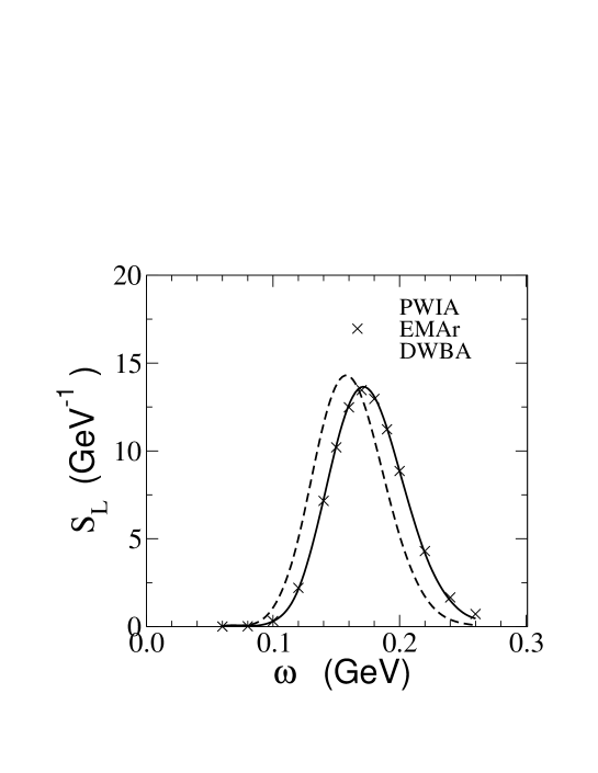
Figure 5: Response function for the 1s shell based on the PWIA, EMAr and full 6D calculations for ²⁰⁸Pb at E_i = 500 Mev and $q=550$ MeV/c.

The DWBA and EMAr results agree very well for the shift of the peak response relative to the peak of the PWIA response function. This is confirmed by fits of each of these responses to the EMA form of Eq. (3) using the parameters shown in Table 1. The shift of the 1s-shell peak response relative to the PWIA peak response is fit by $\delta k$ of -22.0 MeV for the full DWBA case (labeled 6D-F_exact in the table) and by -22.0 MeV for the EMAr response function. The magnitude of the peak EMAr response function is about 1.5% lower than that for the DWBA response function as shown by the A fit parameters in the table.

Table 1: EMA fit parameters for the 1s shell response functions at E=500 MeV and $q$=550 MeV/c. $\delta$k is in MeV.

	$~{}\delta$k	$f_{EMA}$	A
$EMAr$	-22.0	0.80	0.985
$6D-F_{exact}$	-22.0	0.80	1.00
$6D-F_{eff}$	-22.0	0.80	1.00

In order to test one of the assumptions of the EMA or EMAr analysis, we also calculated full DWBA cross sections with the form factor and current-conservation factor evaluated at $q_{eff}$ and removed from the integral over the photon momentum. However, the photon propagator was left within the integral. This allows a comparison of results for $S_{L}^{(DWBA)}$ with the nonlocality of the form factor integrated over versus otherwise identical results with the form factor evaluated at the effective momentum transfer and taken out of the integral. In the latter case the form factor simply cancels out of the result. When $S_{L}^{(DWBA)}$ is calculated with the form factor evaluated at $q_{eff}$ and factored out of the integral, thus canceling, the result is fit using the parameters in the line of Table 1 labeled 6D-F_eff. When $S^{(DWBA)}_{L}$ is calculated with the form factor integrated over and then divided out at $q_{eff}$, the result is fit using the parameter values in the line labeled 6D-F_exact in the table. Both calculations are found to produce essentially the same response functions, $S_{L}^{DWBA}$, in the sense that the same fitting parameters describe both equally well. Thus, there is not any evidence for errors associated with evaluating the form factor at $q_{eff}$ and factoring it out of the integral. This is a nontrivial and important result because the form factor reduces the cross sections by about a factor 4 for q=0.55 GeV/c. There would be a significant difference if the form factor evaluated at the momentum transfer of the electron were divided out in Eq.(31) as has been assumed to be the correct procedure in some works. Use of the momentum transfer of the electron, q, versus the effective photon momentum, $q_{eff}$, leads to a difference in cross sections by a factor $\widetilde{G}_{E}^{2}(q^{2}-\omega^{2})/\widetilde{G}_{E}^{2}(q_{eff}^{2}-\omega^{2})\approx 1.23$ for ${}^{208}Pb$ at $q$ = 0.55 GeV/c and $\omega$ = 0.17 GeV. We find very clear evidence from this analysis that the form factor should be evaluated at the effective photon momentum transfer rather than the momentum transfer of the electron when response functions are extracted from data.

We draw the following conclusions from these tests. The EMAr approximation provides a good approximation to the full 6D DWBA analysis. It reproduces the shift of the DWBA response relative to the PWIA response very well, i.e., the momentum shift $\delta$k is the same: ($\delta$k${}^{(6D}=\delta$k^(EMAr)). When the focus factors are kept within the integration over $r$ as in the EMAr analysis, they do not cancel precisely with the prefactor $Q^{4}/Q^{4}_{eff}$. The $r$-integration provides a normalization reduction of about 1.5%, i.e., A = 0.985 in fits of the EMAr results to the EMA form. In the 6D analysis with the nonlocality of the photon propagator also included in the integration over photon momentum, but everything else the same as in the EMAr calculation, there is no normalization correction, i.e., A = 1.00 in fits to the EMA form. We conclude that the nonlocality of the photon propagator produces a normalization 1.5% greater than the normalization of the EMAr response function: ( $R_{L}^{(6D)}\approx 1.015R_{L}^{(EMAr)}$ ), thus canceling the normalization reduction of the EMAr result. In order to include the nonlocality of the photon propagator, the normalization of the EMAr response for ${}^{208}Pb$ should be increased by the factor 1.015. It then agrees with the normalization of the full DWBA result because the nonlocality of the photon propagator cancels the reduction that arises in the EMAr result. The renormalized EMAr result is found to give excellent agreement with the full DWBA results for both the shift and the normalization. When the nucleon form factor and current-conservation factors also are kept in the integration over photon momentum, there is no additional change of the normalization compared with evaluating those factors at $q_{eff}$.

III.4 Comparison of EMAr and EMA calculations

The three-dimensional integral of Eq. (17) is dominated by a stationary phase point that may be obtained by approximating the eikonal phase $\chi({\bf r})\approx\chi(0)+{\bf r}\cdot\nabla\chi(0)+\cdots$. The effective momentum is then

$${\bf q}_{eff}={\bf q}+\nabla\chi(0)$$ (32)

and the integral for the time-component of the current takes the form [using $h_{e}^{0}=cos\frac{1}{2}\theta_{e}$]

$${\cal M}^{0,EMAr^{\prime}}_{nlm}=cos\frac{1}{2}\theta_{e}e^{i\chi(0)}\int d^{3}re^{i({\bf q}_{eff}-{\bf p})\cdot{\bf r}}f_{i}({\bf r})f_{f}({\bf r})\psi_{nlm}({\bf r}).$$ (33)

Generally it is found that the use of $q_{eff}$ overestimates the Coulomb corrections unless $\nabla\chi(0)$ is reduced by a factor in order to simulate an average value over the nucleus, i.e.,

$${\bf q}_{eff}={\bf q}+f_{EMA}\nabla\chi(0).$$ (34)

We refer to this stationary-point analysis with the full r-dependence of the focus factors left within the integral as EMAr’ and use $f_{EMA}$ = 0.8, as is consistent with fits of the EMAr result. When the focus factors are also approximated using

$$f_{i}({\bf r})f_{f}({\bf r}) \approx \Big{(}1-f_{EMA}V(0)/k_{i}\Big{)}\Big{(}1-f_{EMA}V(0)/k_{f}\Big{)}$$ (35)

$$= \frac{k_{i,eff}k_{f,eff}}{k_{i}k_{f}}$$

then they are cancelled by the $1/Q_{eff}^{2}$ factor in the response function. That approximation leads to the usual EMA result,

$${\cal M}^{0,EMA}_{nlm} =cos\frac{1}{2}\theta_{e}\frac{k_{i,eff}k_{f,eff}}{k_{i}k_{f}}\psi_{nlm}({\bf q}_{eff}-{\bf p}).$$ (36)

The effective momentum approximations provide a good reproduction of the full $6D$ analysis for both the longitudinal response function, $R_{L}$, and the transverse response function, $R_{T}$, as shown in Figures 6 and 7. The EMAr’ stationary-point analysis using $f_{EMA}=0.8$ produces essentially the same results as the EMAr that includes the integration over the variation of $\chi({\bf r})$. The EMA result is also very close to the results based on EMAr and EMAr’. Thus, it is clear that the integration over r that is incorporated in the EMAr analysis provides results that differ only in the fine details. The usual EMA analysis is almost as good once one has in hand a reasonable value of $f_{EMA}$ to use. Some numerical values are given in Table 2 in order to provide a more quantitative comparison of the approximations with the $6D$ calculation.

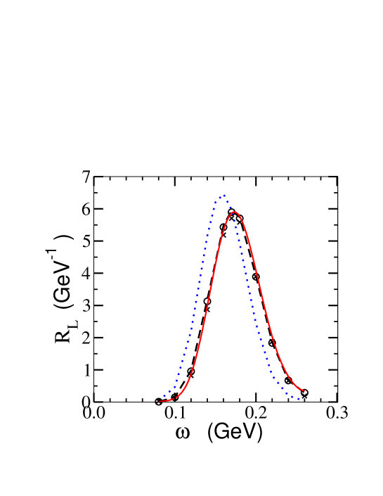
Figure 6: Longitudinal response function for the 1s-shell of ${}^{208}Pb$ based on the PWIA (dotted line), EMA (o symbols), EMAr’ (dash line), EMAr (solid line) and full 6D calculations (x symbols) at E_i = 500 Mev and $q=550$ MeV/c.

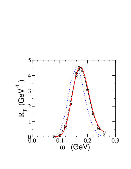
Figure 7: Transverse response function for the 1s-shell ${}^{208}Pb$ based on the PWIA (dotted line), EMA (o symbols), EMAr’ (dash line), EMAr (solid line) and full 6D calculations (x symbols) at E_i = 500 Mev and $q=550$ MeV/c.

Table 2: Numerical values for $R_{L}$ and $R_{T}$ for the 1s-shell of ${}^{208}Pb$ at E=500 MeV and $q$=550 MeV/c.

$\omega$	$R_{L}^{(PWIA)}$	$R_{L}^{(EMA)}$	$R_{L}^{(EMAr)}$	$R_{L}^{(EMAr^{\prime})}$	$R_{L}^{(6D)}$
0.10	0.47	0.15	0.12	0.15	0.13
0.16	6.5	5.4	5.3	5.5	5.2
0.20	2.5	3.9	4.1	3.9	3.9
$\omega$	$R_{T}^{(PWIA)}$	$R_{T}^{(EMA)}$	$R_{T}^{(EMAr)}$	$R_{T}^{(EMAr^{\prime})}$	$R_{T}^{(6D)}$
0.10	0.33	0.11	0.09	0.11	0.09
0.16	4.6	4.1	4.1	4.2	3.9
0.20	1.9	3.1	3.2	3.1	3.1

IV Cross section calculations

Numerical calculations using the EMAr analysis have been performed including all shells of shell-model wave functions with the harmonic oscillator parameter adjusted so that the correct nuclear charge radius is obtained. Table 3 shows the parameter values used. Harmonic oscillator wave functions are used for the shell model. In coordinate space they are

$$\psi_{nlm}({\bf r})=NY_{lm}(\Omega_{r})r^{l}\,_{1}F_{1}(-(n-l)/2,l+3/2,r\sqrt{2}/\beta)\,e^{-(r/\beta)^{2}}$$ (37)

with normalization constants $N$ determined by $\int d^{3}r|\psi({\bf r})|^{2}=1$. Furthermore, $Y_{lm}$ are the well known spherical harmonics and ${}_{1}F_{1}$ the confluent hypergeometric functions.

Table 3: Parameters used in calculations: $\beta$ is the harmonic oscillator parameter; $V_{0}$ and $R$ are the Coulomb potential parameters.

Nucleus	$~{}\beta$(fm)	$V_{0}$ (GeV)	$R$ (fm)
${}^{208}Pb$	3.564	0.0256	7.10
${}^{56}Fe$	2.854	0.0124	3.97

Neutron contributions to cross sections are required in order to include the magnetic scattering. They are assumed to be proportional to the proton contributions and are included by using suitable form factors, i.e.,

$$\widetilde{G}_{E}^{2}\longrightarrow\widetilde{G}_{Ep}^{2}+\frac{N}{Z}\widetilde{G}_{En}^{2},$$

$$G_{M}^{2}\longrightarrow G_{Mp}^{2}+\frac{N}{Z}G_{Mn}^{2}$$ (38)

times the proton contributions, where subscripts $p$ and $n$ refer to the proton and neutron, respectively. Dipole form factors $1/(1+Q^{2}/0.71GeV^{2})^{2}$ are used for the variation of $F_{1}$ and $F_{2}$ with $Q^{2}$.

Figure 8 shows cross sections for ${}^{208}Pb$ at 500 MeV electron energy. The momentum transfer is held fixed at 550 MeV/c and therefore the scattering angle varies with energy loss $\omega$ from about $70^{\small o}$ to about $100^{\small o}$. The figure shows the plane-wave (PWIA) cross sections as light lines and the EMAr results for Coulomb distorted cross sections as heavy lines. Generally the Coulomb corrections shift the peaks to larger energy loss. In our calculations, the average binding energy of 8 MeV was used for all shells. Figure  9 shows similar cross sections at 800 MeV electron energy with the momentum transfer held fixed at 900 MeV/c. In this case the scattering angle varies from about $70^{\small o}$ to about $105^{\small o}$. At the higher momentum transfer, the longitudinal cross section is seen to be a small fraction of the total cross section even without the pionic contributions.

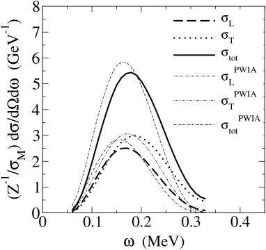
Figure 8: Ratio of EMAr and PWIA longitudinal, transverse and total cross sections to Z times the Mott cross section for 500 MeV electron scattering from ${}^{208}Pb$ at q=550 MeV/c.

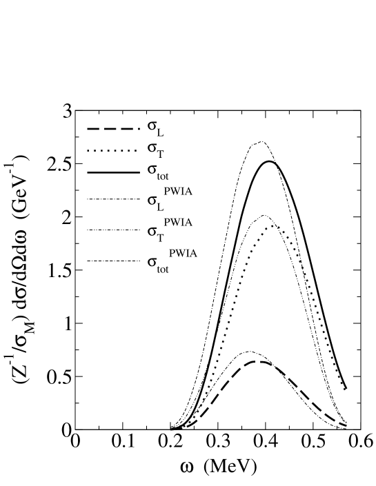
Figure 9: Ratio of EMAr and PWIA longitudinal, transverse and total cross sections to Z times the Mott cross section for 800 MeV electron scattering from ${}^{208}Pb$ at q=900 MeV/c.

Longitudinal response functions for ²⁰⁸Pb are shown in Figure 10. In this figure, the PWIA response functions shown obey the Coulomb sum rule in the form

$$\int d\omega\frac{S_{L}^{PWIA}(\omega,q)}{1+\frac{\omega^{2}}{4M(M+\omega}}=1,$$ (39)

where the kinematical factor in the denominator cancels the kinematical factors due to wave functions normalizations and currents. The correction is modest: the denominator factor is about 1.01 at $\omega=0.2$ GeV and 1.03 at $\omega=0.4$ GeV.

Note that the contributions owing to correlations in the nuclear wave functions are omitted in our calculations. If they are small at the q values shown, the Coulomb sum rule should be satisfied approximately. Our wave functions are approximate and final-state interactions of the knocked-out nucleon have been omitted. Cross sections presented in this work are not expected to be very close to experimental results, however, the nuclear model used is expected to be adequate for testing the accuracy with which Coulombic effects can be removed.

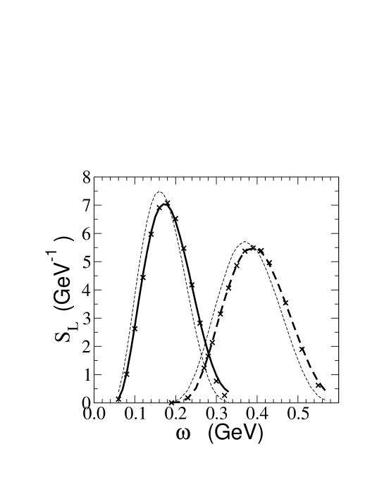
Figure 10: EMAr longitudinal response functions divided by Z and the nucleon form factor for ²⁰⁸Pb at E_i = 500 Mev and $q=550$ MeV/c (solid line) and at E_i = 800 Mev and $q=900MeV/c$ (dashed line). The corresponding PWIA response functions without Coulomb effects included are shown by the light dashed lines. Fits of the response functions using Eq. (3) are shown by the $\times$ symbols and the parameters of the fits are given in Table 4.

We have fit the EMAr longitudinal response functions to the EMA form as in Eq. (3) using the same value of $q_{eff}$ in the prefactor of Eq. (30) as in the PWIA response function. The fits of the EMAr response function based on all shells yield similar values for $A$ and a little smaller values for $\delta$k compared with fits of the 1s shell response function. The fit parameters are summarized in Table 4.

Table 4: EMA fit parameters for the EMAr response functions at energy $E$ in GeV and momentum transfer $q$ in GeV/c. The value of $\delta$k is in MeV.

Nucleus	$E$	$q$	$\delta$k	$f_{EMA}$	$A^{EMAr}$	$A^{DWBA}$
${}^{208}Pb$	0.5	0.55	-21.0	0.82	0.98	$\approx$1.00
${}^{208}Pb$	0.8	0.90	-19.5	0.76	0.985	$\approx$1.00
${}^{58}Fe$	0.5	0.55	-8.8	0.71	0.99	$\approx$1.00
${}^{58}Fe$	0.8	0.90	-9.5	0.77	1.00	$\approx$1.00

Accounting for the nonlocality of the photon propagator as in the results based on the ${}^{208}Pb$ 1s-shell DWBA response, the $A^{EMAr}$ factors are renormalized by the factor 1.015 to estimate factors $A^{DWBA}$ for a full DWBA analysis that includes all shells. Our results support the use of the EMA fits of experimental data as in Eq. (3) using $A=1$. The $f_{EMA}$ factors are a little smaller when all shells are included. That is understandable because higher shells include ones with wave functions that vanish at $r=0$. For those shells, the distortion effects in the electron waves contribute at radii away from $r=0$ where the Coulomb potential is weaker. The results for the 1s shell show that both EMAr and DWBA yield the same value of $\delta$k. The momentum shifts should be equal also for response functions based on the sum over all shells.

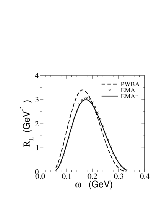
Figure 11: EMAr longitudinal response functions divided by Z for ²⁰⁸Pb at E_i = 500 Mev and $q=550$ MeV/c (solid line). The corresponding PWIA response function without Coulomb effects included is shown by the dashed line and the EMA calculation using $f_{EMA}=0.8$ and $A=1.0$ is shown by the $\times$ symbols.

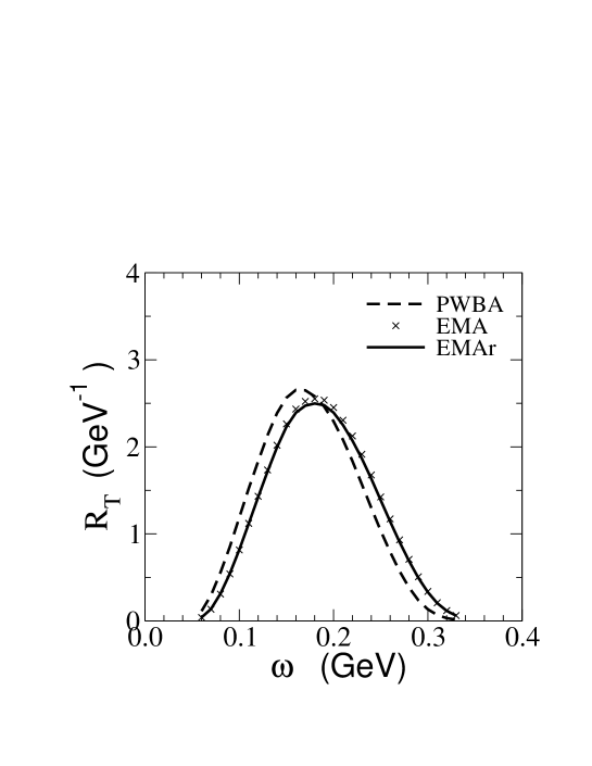
Figure 12: EMAr transverse response functions divided by Z for ²⁰⁸Pb at E_i = 500 Mev and $q=550$ MeV/c (solid line). The corresponding PWIA response function without Coulomb effects included is shown by the dashed line and the EMA calculation using $f_{EMA}=0.8$ and $A=1.0$ is shown by the $\times$ symbols.

Figures 11 and 12 show the longitudinal and transverse response functions $R_{L}$ and $R_{T}$ that do not have form factors divided out for Pb at q=550 MeV/c. Results are shown for the PWIA, EMA and EMAr calculations, where the EMA results are not a fit but rather are a straightforward calculation using $f_{EMA}=0.8$ and $A=1.0$. The Coulomb effects of the EMAr analysis are well approximated by the EMA calculation. As has been discussed, the overall magnitude of the EMA response is higher than the EMAr response by about 2% because the $A$ parameter has not been used.

Figure 13 shows cross sections for ${}^{56}Fe$ at 500 MeV electron energy and q= 550 MeV/c and Figure 14 shows cross sections at 800 MeV electron energy and q = 900 MeV/c. Coulomb effects are somewhat smaller for the ${}^{56}Fe$ nucleus because the Coulomb potential is smaller. Response functions for the ${}^{56}Fe$ target are shown in Figure 15. Fits of the response functions to the EMA form of Eq. (3) yield the fitting parameters shown in Table 4. The shifts are given in this case by $f_{EMA}=$ 0.71 (500 MeV) and 0.77 (800 MeV).

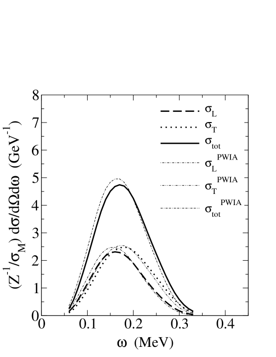
Figure 13: Ratio of EMAr and PWIA longitudinal, transverse and total cross sections to Z times the Mott cross section for 500 MeV electron scattering from ${}^{56}Fe$ at q=550 MeV/c.

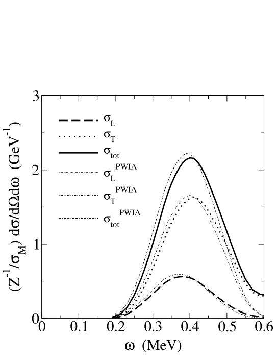
Figure 14: Ratio of EMAr and PWIA longitudinal, transverse and total cross sections to Z times the Mott cross sections for 800 MeV electron scattering from ${}^{56}Fe$ at q=900 MeV/c.

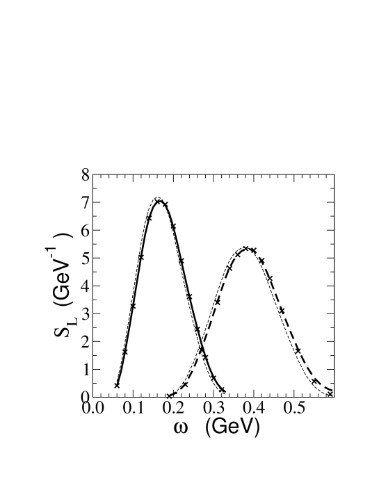
Figure 15: EMAr longitudinal response functions divided by Z and the nucleon form factor for ⁵⁶Fe at E_i = 500 Mev and $q=550$ MeV/c (solid line) and at E_i = 800 Mev and $q=900MeV/c$ (dashed line). The corresponding PWIA response functions without Coulomb effects included are shown by the light dashed lines. Fits of the response functions using Eq. (3) are shown by the $\times$ symbols and values of the fitting parameters are given in Table 4.

V Conclusions

In this work we have tested some assumptions that have been used in the analysis of experimental data for quasielastic scattering from nuclei. The main focus is to use a known nuclear model (in this case the shell model) in order to test how well the Coulomb corrections can be removed from DWBA cross sections using the effective-momentum approximation (EMA). The goal is to extract PWIA response functions from the DWBA cross sections. It is assumed that the Coulomb corrections are not much affected by the nuclear model used.

At the electron beam energies considered in the work, namely 500 MeV and higher, the Coulomb effects in quasielastic scattering from nuclei can be described accurately using the eikonal distorted waves that include higher-order corrections. The eikonal analysis has simplifying features because one can isolate the phases that cause shifts of the electron momenta, the focusing factors and the spin phases that affect the L/T separation. We have used the analytical phases up to order $1/k^{2}$ in the eikonal expansion that were developed in Ref. Tjon&Wallace06 . As one check on the numerics, the eikonal phases were computed two ways: by direct numerical integration of the defining equations and by use of the analytical formulas. Both give the same results. For the cases considered in this work, the eikonal wave functions provide very well converged results. As a check of the three-dimensional integration used in the EMAr analysis, the PWIA results were computed two ways: using analytical Fourier transforms of the nucleon’s bound state wave functions and by three-dimensional numerical integration. The latter calculations are the same as those for the EMAr amplitude except that the Coulomb effects are omitted. With suitable integration grids the results are essentially the same at an accuracy better than 1% near the peak of response functions and errors at larger $\omega$ can be 1% or 2% of the peak value of the response function. Generally the errors in numerical results are insignificant in the plots.

Full DWBA computations are extremely time consuming. An approximation called EMAr is used to simplify the analysis. The EMAr analysis evaluates the full r-dependence of the eikonal distorted waves but approximates the hard-photon propagator and the form factor in the nucleon current by evaluating them at the effective momentum, $q_{eff}$. Tests of the EMAr against the full DWBA analysis were carried out for the response function of the 1s shell of ²⁰⁸Pb. Those tests showed that the EMAr produces close agreement with the DWBA. Moreover, the assumption that one should remove the nucleon form factor (which is integrated over in the DWBA analysis) by evaluating it at $q_{eff}$ was found to be justified with better than 1% accuracy. This should be compared with large differences in cross sections when the form factor is evaluated at $q$, the momentum transfer of the electron, instead of $q_{eff}$. We find clear evidence that the form factor should be evaluated at the effective momentum when it is divided out of experimental cross sections in order to check the Coulomb sum rule.

The analysis of Bates experimental data in Ref. Williamson97 uses the form factor at $q$ rather $q_{eff}$ for a ${}^{40}Ca$ nucleus. Results for the Coulomb sum rule are about 0.8-0.9 compared with the expectation of unity. If $q_{eff}$ were used in the analysis, the Bates results for the Coulomb sum rule would be increased by about 5%, thus making them closer to unity. The analysis of Saclay experimental data in Refs. Meziani84 ; Meziani85 uses form factors at $q_{eff}$. Significantly lower values for the Coulomb sum rule are found based on the Saclay analysis. The differences between the Bates and Saclay results are much larger than can be attributed to Coulomb corrections.

We find that the spin phases in electron wave functions produce very small effects at energies of 500 MeV or higher. The helicity matrix elements that involve the spin phases are very close to those of a PWIA analysis for quasi-elastic scattering. Consequently, the Rosenbluth separation extracts response functions $R_{L}^{expt}$ and $R_{T}^{expt}$ that are accurate in the sense that they correspond very closely to the distorted wave matrix elements of the longitudinal and transverse parts of the currents.

The effects of the distorted waves on the longitudinal response function are twofold: 1.) for electron scattering they shift the peak of the response functions towards larger values of the energy loss, $\omega$, and 2.) they distort the shapes of the response functions, more so for the inner shells than the outer ones. However, reasonably accurate fits of the distorted response functions can be obtained using the EMA fitting procedure of Eq. (3). The momentum shift parameter $\delta k$ is found to be given by $f_{EMA}\approx 0.80$, for both the ${}^{208}Pb$ and ${}^{56}Fe$ nuclei, i.e., $\delta k\approx 0.80V_{c}(0)$, where $V_{c}(r)$ is the Coulomb potential. More precise values are given in Table 4. The normalization parameter $A$ is equal to 1.00 within one or two percent. The uncertainty arises because the normalization for the sum over shells has been calculated based on the full DWBA for the 1s-shell of ${}^{208}Pb$ and because the shape of the distorted response function differs a little from the shape of the PWIA response function for $\omega$ significantly away from the peak. Therefore fits to the PWIA shape cannot reproduce the response precisely. Note that the good agreement of $f_{EMA}$ and $A$ for ²⁰⁸Pb and ⁵⁶Fe demonstrates that the Coulomb corrections do not depend significantly on the nuclear model. Note also that the analysis of experimental data using a fit as in Eq. (3) tends to give more accurate results for $R_{L}^{(PWIA)}$ at the peak of the response because that is controlled by $\delta k$ and less accurate results away from the peak because of the distortion of the shape.

Estimates of longitudinal, transverse and total cross sections have been calculated using shell model wave functions for ${}^{208}Pb$ and ${}^{56}Fe$ at $q$ = 0.55 GeV/c and $q$ = 0.8 GeV/c. These kinematical conditions match the ones used in a recent experiment at Jlab. Because final-state interactions, correlations and pion production have been omitted, the calculated cross sections may differ significantly from experimental cross sections. Nevertheless the Coulomb corrections should be reliable at the level of a few percent.

Coulomb corrections are notoriously difficult to calculate and our calculations refute claims that may be found in the literature. For example, Ref. Kim05 claims that the EMA procedure is not accurate for the longitudinal response at 485 electron energy and $60^{o}$ scattering angle for a ${}^{208}Pb$ target. The basis for the claim is that significant differences are found between EMA results and results based on an ad-hoc DWBA analysis that has been used extensively. We find that the EMA with appropriate parameters can describe the 1s-shell DWBA or all-shells EMAr results very well at essentially the same kinematics. We wish to emphasize that all of our numerics are under good control and various consistency checks have been made that give confidence in the results reported herein.

References

- (1) R. Altemus, et al., Phys. Rev. Lett. 44, 965 (1980).
- (2) M. Deady, et al., Phys. Rev. C 28, 631 (1983).
- (3) A. Hotta, et al., Phys. Rev. C 30, 87 (1984).
- (4) M. Deady, C. F. Williamson, P. D. Zimmerman, R. Altemus and R. R. Whitney, Phys. Rev. C 33, 1897 (1986).
- (5) C. C. Blatchley, et al., Phys. Rev. C 34, 1243 (1986).
- (6) S. A. Dytman, A. M. Bernstein, K. I. Blomqvist, T. J. Pavel, B. P. Quinn, R. Altemus, J. S. McCarthy, G. H. Mechtel, T. S. Ueng and R. R. Whitney, Phys. Rev. C 38, 800 (1988).
- (7) K. Dow, et al., Phys. Rev. Lett. 61, 1706 (1988).
- (8) T. C. Yates, et al., Phys. Lett. B 312, 382 (1993).
- (9) C. Williamson, et al., Phys. Rev. C 56, 3152 (1997).
- (10) P. Barreau, et al., Nucl. Phys A402, 515 (1983).
- (11) Z.-E. Meziani, et al., Phys. Rev. Lett. 52, 2130. (1984).
- (12) Z.-E. Meziani, et al., Phys. Rev. Lett. 54, 1233 (1985).
- (13) C. Marchand, et al., Phys. Lett. B 153, 29 (1985).
- (14) A. Zghiche, et al., Nucl. Phys. A572, 513 (1994).
- (15) P. Guéye, et al., Phys. Rev. C 60, 044308 (1999).
- (16) D. T. Baran, et al., Phys. Rev. Lett. 61, 400 (1988).
- (17) J. P. Chen, et al., Phys. Rev. Lett. 66, 1283 (1991).
- (18) Z.-E. Meziani, et al., Phys. Rev. Lett. 69, 41 (1992).
- (19) O. Benhar, D. Day and I. Sick, Rev. Mod. Phys. 80, 189 (2008).
- (20) G. Co and J. Heisenberg, Phys. Lett. B 197, 489 (1987).
- (21) Yanhe Jin, D. S. Onley and L. E. Wright, Phys. Rev. C 45, 1311 (1992); 45, 1333 (1992); 50, 168 (1994).
- (22) J. M. Udias, P. Sarriguren, E. Moya de Guerra, E. Garrido and J. A. Caballero, Phys. Rev. C 48, 2731 (1993).
- (23) J. M. Udias, P. Sarriguren, E. Moya de Guerra, E. Garrido and J. A. Caballero, Phys. Rev. C 51, 3246 (1995).
- (24) K. S. Kim, L. E. Wright and D. A. Resler, Phys. Rev. C64, 044607 (2001).
- (25) D. R. Yennie, F. L. Boos, Jr., and D. G. Ravenhall, Phys. Rev. 137, 882 (1965).
- (26) F. Lenz and R. Rosenfelder, Nucl. Phys. A176, 513 (1971).
- (27) R. Rosenfeler, Ann. Phys. (N.Y.) 128, 188 (1980).
- (28) W. Czyz and K. Gottfried, Ann. Phys. (N.Y.) 25, 47 (1963).
- (29) A. Baker, Phys. Rev. D6, 3469 (1972).
- (30) C. Giusti and F. D. Pacati, Nucl. Phys. A473, 717 (1987).
- (31) C. Giusti and F. D. Pacati, Nucl. Phys. A486, 461 (1988).
- (32) A. Aste, K. Hencken, J. Jourdan, I. Sick and D. Trautmann, Nucl. Phys. A743, 259 (2004).
- (33) A. Aste and J. Jourdan, Europhys. Lett. 67, 753 (2004).
- (34) M. Traini, Nucl. Phys. A694, 325 (2001).
- (35) M. Traini, S. Turck-Chiéze and A. Zghiche, Phys. Rev. C 38, 2799 (1988).
- (36) J. Morgenstern and Z.-E. Meziani, Phys. Lett. B 515, 269 (2001).
- (37) J. A. Tjon and S. J. Wallace, Phys. Rev. C74, 064602 (2006).
- (38) J. A. Tjon and S. J. Wallace, arXiv:0805.4396, 2008, to be published in Indian Journ. Phys..
- (39) A. Aste, arXiv:0710.1261v3, 2008.
- (40) Y. Horikawa, F. Lenz, N. C. Mukhopadhyay, Phys. Rev. C22, 1680 (1980).
- (41) O. Benhar, A. Fabrocini, S. Fantoni, Nucl. Phys. A505, 267 (1989).
- (42) I. Sick, Prog. Part. Nucl. Phys. 59, 447 (2007).
- (43) J. W. Van Orden and T. W. Donnelly, Ann. Phys. (NY) 131, 451 (1981); C. R. Chinn, A. Picklesimer and J. W. van Orden, Phys. Rev. C40, 790 (1989).
- (44) M. J. Dekker, P. J. Brussaard and J. A. Tjon, Phys. Lett. B 266, 249 (1991); Phys. Lett. B 289, 255 (1992); Phys. Rev. C49, 2650 (1994); Phys. Rev. C51, 1393 (1995).
- (45) H. de Vries, C. W. de Jager, C. de Vries, Atomic Data and Nucl. Data Tables 36, 495 (1987).
- (46) K. S. Kim and L. E. Wright, Phys. Rev. C72, 064607 (2005).