Time-dependent density-functional theory for electronic excitations in materials: basics and perspectives

Abstract

Time-dependent density-functional theory (TDDFT) is widely used to describe electronic excitations in complex finite systems with large numbers of atoms, such as biomolecules and nanocrystals. The first part of this paper will give a simple and pedagogical explanation, using a two-level system, which shows how the basic TDDFT formalism for excitation energies works. There is currently an intense effort underway to develop TDDFT methodologies for the charge and spin dynamics in extended systems, to calculate optical properties of bulk and nanostructured materials, and to study transport through molecular junctions. The second part of this paper highlights some challenges and recent advances of TDDFT in these areas. Two examples are discussed: excitonic effects in insulators and intersubband plasmon excitations in doped semiconductor quantum wells.

I Introduction

Many important areas of experimental and theoretical physics, chemistry, and materials science require an understanding of the electronic excitations of atomic or molecular systems, nanostructures, mesoscopic systems, or bulk materials.Carter2008 ; Koch2006 ; Scholes2006 ; Chelikowsky2003 A wide variety of spectroscopic techniques is being used to characterize the electronic structure and dynamics of these systems by probing their excitation spectra. The performance of any nanoelectronic device, such as a molecular junction, is dominated by its electronic excitations. Nitzan2003 ; Koentopp2008

Time-dependent density-functional theory (TDDFT) TDDFT_book is an increasingly popular, universal approach to electronic dynamics and excitations. Just like ground-state density-functional theory (DFT), which is based on a set of rigorous theorems HK ; KS proving a one-to-one correspondence between ground-state densities and potentials, there is a similar existence theorem for TDDFT, due to Runge and Gross, Runge1984 which establishes the time-dependent density as a fundamental variable.

The usage of TDDFT as a practical tool to calculate excitation energies started in the mid-90’s with the groundbreaking work of Petersilka et al. Petersilka1996 and Casida. Casida1996 In the Casida-formalism, the excitation energies are obtained from the following eigenvalue problem:

$$\left(\begin{array}[]{cc}{\bf A}&{\bf K}\\ {\bf K}^{*}&{\bf A}^{*}\end{array}\right)\left(\begin{array}[]{c}{\bf X}\\ {\bf Y}\end{array}\right)=\omega\left(\begin{array}[]{cc}-{\bf 1}&{\bf 0}\\ {\bf 0}&{\bf 1}\end{array}\right)\left(\begin{array}[]{c}{\bf X}\\ {\bf Y}\end{array}\right),$$ (1)

where the matrices $\bf A$ and $\bf K$ are defined as follows:

$$A_{ia\sigma,i^{\prime}a^{\prime}\sigma^{\prime}}=\delta_{ii^{\prime}}\delta_{aa^{\prime}}\delta_{\sigma\sigma^{\prime}}(\varepsilon_{a\sigma}-\varepsilon_{i\sigma})+K_{ia\sigma,i^{\prime}a^{\prime}\sigma^{\prime}}$$ (2)

and

$$K_{ia\sigma,i^{\prime}a^{\prime}\sigma^{\prime}}=\int d^{3}r\int d^{3}r^{\prime}\varphi^{*}_{i\sigma}({\bf r})\varphi_{a\sigma}({\bf r})\left[\frac{1}{|{\bf r}-{\bf r}^{\prime}|}+f_{\rm xc,\sigma\sigma^{\prime}}({\bf r},{\bf r}^{\prime},\omega)\right]\varphi_{i^{\prime}\sigma^{\prime}}({\bf r}^{\prime})\varphi^{*}_{a^{\prime}\sigma^{\prime}}({\bf r}^{\prime}).$$ (3)

Here, $\varphi_{i\sigma}$ and $\varepsilon_{i\sigma}$ are the Kohn-Sham orbitals and eigenvalues coming from a self-consistent ground-state DFT calculation; we use the standard convention that $i,i^{\prime},\ldots$ are indices of occupied orbitals and $a,a^{\prime},\ldots$ refer to unoccupied orbitals. $f_{\rm xc,\sigma\sigma^{\prime}}({\bf r},{\bf r}^{\prime},\omega)$ is the so-called exchange-correlation (XC) kernel,Gross1985 which is in general a frequency-dependent quantity, but in practice is often approximated using frequency-independent expressions. This is known as the adiabatic approximation.

The eigenvalues $\omega$ of Equation (1) are, in principle, the exact excitation energies of the system, provided one would start from an exact Kohn-Sham ground-state calculation and then use the exact $f_{\rm xc,\sigma\sigma^{\prime}}$. In practice, of course, static and dynamical XC functionals need to be approximated. The formalism of Equations (1)-(3) can also be recast in the shape of an eigenvalue problem for the squares of the excitation energies:

$$\sum_{a^{\prime}i^{\prime}\sigma^{\prime}}\left[\delta_{ii^{\prime}}\delta_{aa^{\prime}}\delta_{\sigma\sigma^{\prime}}\omega_{ia\sigma}^{2}+2\sqrt{\omega_{ia\sigma}\omega_{i^{\prime}a^{\prime}\sigma^{\prime}}}K_{ia\sigma,i^{\prime}a^{\prime}\sigma^{\prime}}\right]\xi_{a^{\prime}i^{\prime}\sigma^{\prime}}=\omega^{2}\xi_{ai\sigma}\>,$$ (4)

where $\omega_{ia\sigma}=\varepsilon_{a\sigma}-\varepsilon_{i\sigma}$.

This TDDFT formalism for excitation energies has become very popular for practical applications, and is nowadays implemented as an integral part of several widely used software packages in theoretical chemistry. Furche2002 Overall, TDDFT affords a unique balance between accuracy and efficiency, allowing the user to study systems that would be impossible to treat with traditional wavefunction methods, for example in all-electron studies of the photochemistry of large biomolecules. Marques2005 ; Varsano2006 To describe localized and delocalized electronic excitations in large conjugated and aggregated molecules, TDDFT has also been used along semiempirical Hamiltonian models or approaches based on the Kohn-Sham density matrix such as the collective electronic oscillator (CEO) model. Tretiak2002 ; Berman2003

The broad spectrum of applications of TDDFT for excited states has been recently reviewed by Elliott et al. Elliott2007 From the large body of available literature, the following trends for molecules have emerged. Transition frequencies, calculated with standard gradient-corrected XC functionals are typically good to within 0.4 eV. Excited-states structural properties such as bond lengths, vibrational frequencies and dipole moments are essentially as good as those of ground-state calculations (about 1 % for bond lengths, and about 5 % for dipoles and vibrational frequencies). Most importantly for large systems, the computational costs scale as $N^{3}$, versus $N^{5}$ for wavefunction methods of comparable accuracy (eg CCSD, CASSCF).

While there exist efficient iterative algorithms for solving the full eigenvalue problem (1), it is nevertheless useful to consider approximations, since these can lead to further insight. The Tamm-Dancoff approximation (TDA) neglects the off-diagonal matrices $\bf K$ in Equation (1), which results in the simpler eigenvalue problem

$${\bf AX}=\omega_{\rm TDA}{\bf X}\>.$$ (5)

Physically, the TDA is the TDDFT analog of the configuration interaction singles (CIS) method.Hirata1999 The TDA has some technical advantages away from ground-state equilibrium geometry, as discussed by Casida et al. in Ref. TDDFT_book, .

In an even more drastic approximation, Equation (4) is truncated down to a $1\times 1$ matrix. This yields the so-called small-matrix approximation (SMA), Appel2003 which for spin-saturated systems is given by

$$\omega^{2}_{\rm SMA}=\omega_{ia}^{2}+4\omega_{ia}K_{ia,ia}.$$ (6)

This can be further approximated if the correction to the bare Kohn-Sham excitation energy $\omega_{ia\sigma}$ is small, which is known as single-pole approximation (SPA):Petersilka1996 ; Appel2003

$$\omega_{\rm SPA}=\omega_{ia}+2K_{ia,ia}.$$ (7)

This approximation can also be viewed as a TDA for a two-level system. Below, we shall present an alternative, more direct derivation of the SMA and SPA. It turns out that these two approximations perform surprisingly well for simple closed-shell atomic systems. Vasiliev1999 This might perhaps be viewed as merely a curiosity — after all, one can describe such systems with the full Casida TDDFT formalism without resorting to any approximation. However, the SMA and SPA can prove very useful for situations such as extended systems where the full Casida formalism cannot be easily applied, and we shall hence focus on such cases.

The purpose of this paper is to present a discussion of simplified TDDFT approaches to excitation energies in bulk materials and quantum wells. We will begin with a simple and pedagogical derivation of the small-matrix and single-pole approximation for a two-level Kohn-Sham system. We will then show how these expressions can be easily modified and generalized for the case of collective excitations in extended systems. In this way, one can arrive at a simple treatment of excitonic effects in bulk insulators, and plasmon-like excitations in doped semiconductor nanostructures. Some examples will be discussed.

II Excitation energies of a two-level Kohn-Sham system

Let us consider a two-level system consisting of two orbitals $\varphi_{1}({\bf r})$ and $\varphi_{2}({\bf r})$ which are eigenstates of the static Kohn-Sham Hamiltonian

$$H^{0}=-\frac{\hbar^{2}\nabla^{2}}{2m}+V_{\rm ext}({\bf r})+\int d^{3}r\frac{n_{0}({\bf r})}{|{\bf r}-{\bf r}^{\prime}|}+V_{\rm xc}[n_{0}]({\bf r})\>,$$ (8)

where $V_{\rm xc}$ is the exchange-correlation (xc) potential, a functional of the ground-state density $n_{0}({\bf r})$. We assume that $\varphi_{1}$ is doubly occupied and $\varphi_{2}$ is empty.

Now consider a weak perturbation $\lambda H^{\prime}({\bf r},t)$ acting on the system. According to time-dependent perturbation theory, the time evolution of the system is given by

$$\varphi({\bf r},t)=c_{1}(t)\varphi_{1}({\bf r})+\lambda c_{2}(t)\varphi_{2}({\bf r})\>.$$ (9)

Let us construct the density matrix of the system as follows:

$$\rho(t)=\left(\begin{array}[]{cc}\rho_{11}&\lambda\rho_{12}\\ \lambda\rho_{21}&\lambda^{2}\rho_{22}\end{array}\right)=\left(\begin{array}[]{cc}|c_{1}|^{2}&\lambda c_{1}^{*}c_{2}\\ \lambda c_{1}c_{2}^{*}&\lambda^{2}|c_{2}|^{2}\end{array}\right),$$ (10)

where we explicitly indicate the order of the perturbation through orders of $\lambda$. The density matrix obeys the following equation of motion:

$$\dot{\rho}=-i[H,\rho]=-i[H^{0}+\lambda H^{\prime}(t),\rho].$$ (11)

Dropping terms of order $\lambda^{2}$, this yields the time evolution of the off-diagonal elements of the density matrix as follows:

$$\dot{\rho}_{12} = -i[(H^{0}_{11}-H^{0}_{22})\rho_{12}-H^{\prime}_{12}\rho_{11}]$$ (12)

$$\dot{\rho}_{21} = i[(H^{0}_{11}-H^{0}_{22})\rho_{21}-H^{\prime}_{21}\rho_{11}],$$ (13)

where $H^{0}_{11}=\int d^{3}r\varphi_{1}({\bf r})H^{0}\varphi_{1}({\bf r})$ and similar for all other matrix elements of $H^{0}$ and $H^{\prime}$. Since $\rho_{11}=1+{\cal O}(\lambda^{2})$, and defining $H^{0}_{22}-H^{0}_{11}=\omega_{21}$ (the bare Kohn-Sham excitation energy), this simplifies to

$$\dot{\rho}_{12} = i[\omega_{21}\rho_{12}+H^{\prime}_{12}]$$ (14)

$$\dot{\rho}_{21} = -i[\omega_{21}\rho_{21}+H^{\prime}_{21}].$$ (15)

Next, we make the ansatz (which will be justified later)

$$\rho_{12}(t)=\tilde{\rho}_{12}(\omega)e^{-i\omega t}+\tilde{\rho}_{12}(-\omega)e^{i\omega t}\>,$$ (16)

and similar for $\rho_{21}$, $H^{\prime}_{12}$, and $H^{\prime}_{21}$. This gives

$$-\omega\tilde{\rho}_{12}(\omega) = [\omega_{21}\tilde{\rho}_{12}(\omega)+\tilde{H}^{\prime}_{12}(\omega)]$$ (17)

$$-\omega\tilde{\rho}_{21}(\omega) = -[\omega_{21}\tilde{\rho}_{21}(\omega)+\tilde{H}^{\prime}_{21}(\omega)]$$ (18)

and an additional two equation for $\tilde{\rho}_{12}(-\omega)$ and $\tilde{\rho}_{21}(-\omega)$ which do not contain any new information. Adding Equations (17) and (18) gives

$$\tilde{\rho}_{12}(\omega)+\tilde{\rho}_{21}(\omega)=-\frac{\tilde{H}^{\prime}_{12}(\omega)}{\omega_{21}+\omega}-\frac{\tilde{H}^{\prime}_{21}(\omega)}{\omega_{21}-\omega}\>.$$ (19)

Let us now consider the perturbing Hamiltonian:

$$H^{\prime}({\bf r},\omega)=\int d^{3}r^{\prime}\left[\frac{1}{|{\bf r}-{\bf r}^{\prime}|}+f_{\rm xc}({\bf r},{\bf r}^{\prime},\omega)\right]\delta n({\bf r}^{\prime},\omega)\>,$$ (20)

where

$$\delta n({\bf r},\omega)=2\varphi_{1}({\bf r})\varphi_{2}({\bf r})[\tilde{\rho}_{12}(\omega)+\tilde{\rho}_{21}(\omega)].$$ (21)

Notice that we do not consider an external perturbation, only the linearized Hartree and XC potentials. We are thus looking for an “eigenmode” of the system in a steady-state. This justifies the ansatz (16) made above. We define the double matrix element

$$F(\omega)=2\int d^{3}r\int d^{3}r^{\prime}\varphi_{1}({\bf r})\varphi_{2}({\bf r})\left[\frac{1}{|{\bf r}-{\bf r}^{\prime}|}+f_{\rm xc}({\bf r},{\bf r}^{\prime},\omega)\right]\varphi_{1}({\bf r}^{\prime})\varphi_{2}({\bf r}^{\prime})\>,$$ (22)

and Equation (19) becomes

$$\tilde{\rho}_{12}(\omega)+\tilde{\rho}_{21}(\omega)=-F(\omega)[\tilde{\rho}_{12}(\omega)+\tilde{\rho}_{21}(\omega)]\left[\frac{1}{\omega_{21}+\omega}+\frac{1}{\omega_{21}-\omega}\right].$$ (23)

Canceling $\tilde{\rho}_{12}+\tilde{\rho}_{21}$ on both sides results in

$$1=-\frac{2\omega_{21}}{\omega_{21}^{2}-\omega^{2}}\>F(\omega)$$ (24)

which gives the final result

$$\omega^{2}=\omega_{12}^{2}+2\omega_{21}F(\omega)\>.$$ (25)

This is the same as the SMA, Equation (6). From the point of view of our two-level system, our derivation shows that the SMA considers the excitation $1\to 2$ as well as the de-excitation $2\to 1$. The SPA, Equation (7), on the other hand, only includes the excitation $1\to 2$ [it is obtained by ignoring the first pole in Equation (23)]. In general, the TDA (5) ignores all de-excitations.

III Optical excitations in bulk insulators

The standard ab-initio treatment of excitation processes in insulators and semiconductors, including correlation-induced screening, is based on many-body Green’s function techniques such as GW and the Bethe-Salpeter equation. Onida2002 However, TDDFT has recently emerged as an alternative, computationally convenient approach to electronic excitation processes in materials. Onida2002 ; Reining ; Kim ; Botti2007 As discussed above, excitation energies can be calculated in principle exactly in TDDFT, provided the XC kernel $f_{\rm xc}({\bf r},{\bf r}^{\prime},\omega)$ is known, and one starts with an exact ground-state calculation. This statement is true not only for finite systems such as molecules, but remains valid for extended systems. In Refs. Onida2002, ; Reining, , an approximate $f_{\rm xc}$ was constructed from many-body Green’s functions, whereas Ref. Kim, uses an exact-exchange approach, including a cutoff in wavevector space which mimics screening of the Coulomb interaction. Bruneval2006 These studies have established that TDDFT is capable of describing excitonic effects in solids, although one has to use XC functionals that go beyond the more common ones such as the adiabatic local-density approximation. TDDFT_book The resulting agreement with experimental data is excellent, Botti2007 but the technical effort is not significantly less than that of standard many-body approaches.

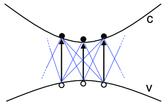
Figure 1: Schematic illustration of interband transitions in an insulator. The thick arrows represent single-particle transitions between the valence (v) and the conduction (c) band. Via dynamical many-body effects, these transitions are coupled (thin blue lines). Excitons can thus be viewed as collective excitations, where the electron-hole interactions involve the entire bands.

In the following, let us for simplicity consider a two-band insulator with valence and conduction band energies $\varepsilon_{\bf k}^{v}$ and $\varepsilon_{\bf k}^{c}$ and associated Bloch functions $\psi_{v{\bf q}}({\bf r})$ and $\psi_{c{\bf q}}({\bf r})$. The single-particle interband transition energies are simply given by $\omega_{\bf k}^{cv}=\varepsilon_{\bf k}^{c}-\varepsilon_{\bf k}^{v}$. A TDDFT formalism for nonlinear ultrafast interband excitations has recently been developed, Turkowski2008 which describes the electron dynamics of a two-band system via a generalization of the semiconductor Bloch equations. This work has shown that TDDFT is capable of producing excitonic signatures in the interband dynamics. We now briefly outline a simpler and more direct TDDFT approach for excitonic binding energies.Turkowski2009

To describe excitonic effects in the interband absorption spectrum of insulators, one needs to go beyond the single-particle picture and include dynamical many-body effects. In TDDFT, this is accomplished through the dynamical XC kernel $f_{\rm xc}({\bf r},{\bf r}^{\prime},\omega)$. Let us illustrate this for the simple case of our two-band insulator. The SPA of Equation (7) refers to two discrete levels, but it can be generalized to two entire bands as follows:

$$\sum_{\bf q}\left[\omega_{\bf q}^{cv}\delta_{\bf kq}+F_{\bf kq}(\omega)\right]\zeta_{\bf q}(\omega)=\omega\zeta_{\bf k}(\omega)\>,$$ (26)

where

$$F_{\bf kq}(\omega)=\frac{2}{\Omega^{2}}\int_{\Omega}d^{3}r\!\int_{\Omega}d^{3}r^{\prime}\>\psi_{c{\bf k}}^{*}({\bf r})\psi_{v{\bf k}}({\bf r})f_{\rm xc}({\bf r},{\bf r}^{\prime},\omega)\psi_{v{\bf q}}^{*}({\bf r}^{\prime})\psi_{c{\bf q}}({\bf r}^{\prime})\>.$$ (27)

Thus, in contrast to the simple SPA Equation (7) which gives an explicit expression for the excitation energy, Equation (26) represents an eigenvalue equation which couples interband transitions of different wavevectors via the coupling matrix $F_{\bf kq}$, Equation (27). This shows explicitly that excitons are collective excitations which involve not only the states at the valence-band maximum and conduction-band minimum (for direct excitons), but the states of the entire bands. A schematic illustration is given in Figure 1. Explicit evaluations of Equations (26) and (27) are currently in progress.Turkowski2009

The TDDFT formalism of Ref. Turkowski2008, can in principle also be used to treat higher-order correlation effects such as biexciton formation. These effects are especially important in the description of the ultrafast nonlinear optical response in semiconductors (bulk and nanostructured). Chemla2001 Such nonlinear effects, which are entirely governed by dynamical correlations, can be expected to put severe demands on the XC functionals, and will be the subject of future studies.

IV Intersubband plasmons in quantum wells

The terahertz frequency regime is scientifically rich, but despite recent progress it is technologically still underdeveloped. ISBbooks Subband spacings in typical III-V quantum wells are of the order of a few tens of meV. Since a photon energy of 10 meV corresponds to a frequency of 2.4 THz, intersubband transitions in quantum wells appear as natural candidates for device applications to fill the “Terahertz gap” in the electromagnetic spectrum. A schematic illustration of intersubband transitions is given in the top panel of figure 2.

The fundamental coupling mechanism between electromagnetic waves and carriers in a doped semiconductor quantum well is through a collective excitation, the so-called intersubband plasmon. To date, most applications of TDDFT linear response theory in quantum wells have been concerned with calculating intersubband plasmon dispersions and linewidths. bloss89 ; jogai91 ; ryan91 ; dobson92 ; marmorkos93 ; ullrich98 ; ullrich01 ; ullrich02 Due to its highly collective nature, and since the dynamics is essentially one-dimensional, intersubband plasmons in quantum wells are an ideal testing ground for new TDDFT approaches. A review of recent applications of TDDFT to the electron dynamics in semiconductor nanostructure is given in Ref. ullrich2006, .

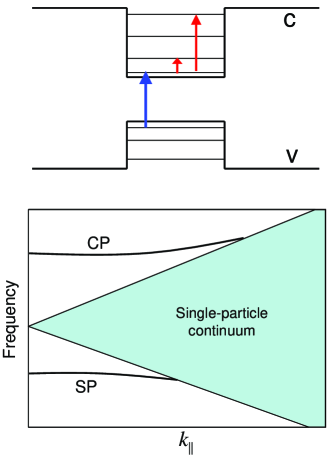
Figure 2: Top: Schematic illustration of interband transitions (blue arrow) and intersubband transitions (red arrows) in a square quantum well. Bottom: Frequency versus in-plane wave vector $k_{||}$ of intersubband excitations in a quantum well. Collective charge and spin plasmon excitations (CP and SP) are separated from the region of incoherent single-particle excitations.

Let us now extend our discussion to include charge as well as spin plasmon excitations. The physical picture of these excitations is that in a charge plasmon the spin-up and spin-down electrons in the quantum well move collectively in phase, whereas in a spin plasmon they move 180 degrees out of phase. These excitations have a dependence on the in-plane wavevector ${\bf k}_{||}$, which is schematically illustrated in Fig. 2. In the $\omega-k_{||}$ plane, one distinguishes an area of incoherent single-particle excitations (also known as Landau damping), and two discrete plasmon branches. The charge plasmon lies above the single-particle regime, and the spin plasmon lies below. Experimentally, this is confirmed via inelastic light scattering spectroscopy.Pinczuk1989

We shall in the following discuss how TDDFT describes the charge and spin plasmons in quantum wells. We adopt the effective-mass approximation for electronic states in doped semiconductor nanostructures. Let $N_{s}$ be the electronic sheet density (the number of electrons per area), which is chosen so that only the lowest subband is occupied. It is assumed that the direction of growth, and thus of quantum confinement, of the quantum well is along the $z$-axis, and electrons are free to move in the $x$-$y$ plane. For simplicity, we consider only the first and the second subband.

The intersubband charge and spin plasmon frequencies $\omega_{c,s}$ are determined by the condition that the following $2\times 2$ matrix equation,

$$\sum_{\sigma^{\prime}}M_{\sigma\sigma^{\prime}}({\bf k}_{||},\omega)h_{\sigma^{\prime}}({\bf k}_{||},\omega)=\lambda h_{\sigma}({\bf k}_{||},\omega)\>,$$ (28)

has eigenvalue $\lambda=1$. The matrix elements are given by

$$M_{\sigma\sigma^{\prime}}({\bf q},\omega) = F_{21}({\bf q},\omega)\left\{\int\!dz\!\int\!dz^{\prime}\left[\frac{2\pi}{q}\>e^{-q|z-z^{\prime}|}+f^{\rm ALDA}_{{\rm xc},\sigma\sigma^{\prime}}(z,z^{\prime})\right]\varphi_{1}(z)\varphi_{2}(z)\varphi_{1}(z^{\prime})\varphi_{2}(z^{\prime})\right.$$ (29)

$$- \frac{i\omega}{\omega_{21}^{2}}\int dz\left[\left(\zeta_{{\rm xc},\sigma\sigma^{\prime}}(z,\omega)+\frac{4}{3}\eta_{{\rm xc},\sigma\sigma^{\prime}}(z,\omega)\right)\left(\nabla_{z}\frac{P(z)}{n(z)}\right)^{2}\right.$$

$$\left.{}+\left.q^{2}\eta_{{\rm xc},\sigma\sigma^{\prime}}(z,\omega)\ \left(\frac{P(z)}{n(z)}\right)^{2}-\frac{\sigma\sigma^{\prime}}{4}\>\Re\rho_{\uparrow\downarrow}(z,\omega)\>P_{z}^{2}(z)\right]\right\},$$

where

$$P(z)=\varphi_{1}(z)\nabla_{z}\varphi_{2}(z)-\varphi_{2}(z)\nabla_{z}\varphi_{1}(z)\>,$$ (30)

and

$$F_{21}({\bf q},\omega)=-\int\frac{d^{2}k}{(2\pi)^{2}}\left\{\frac{f(\varepsilon_{1}+k^{2}/2)}{\omega+\omega_{21}-{\bf q}\cdot{\bf k}+\frac{q^{2}}{2}+i\delta}+\frac{f(\varepsilon_{1}+k^{2}/2)}{-\omega+\omega_{21}-{\bf q}\cdot{\bf k}+\frac{q^{2}}{2}-i\delta}\right\}.$$ (31)

Here, $\varphi_{1}(z)$ and $\varphi_{2}(z)$ are the envelope functions of the first two electronic subbands, $\varepsilon_{1,2}$ are the associated Kohn-Sham energy eigenvalues, and $\omega_{21}=\varepsilon_{2}-\varepsilon_{1}$ is the bare subband spacing (assuming parabolic subbands). A detailed derivation of Equations (29)-(31) will be published elsewhere.Damico2009

The matrix elements $M_{\sigma\sigma^{\prime}}$ of Equation (29) contain various XC contributions. The first XC term features $f_{\rm xc,\sigma\sigma^{\prime}}^{\rm ALDA}(z,z^{\prime})$ in the adiabatic local-density approximation (ALDA). TDDFT_book This term is frequency independent and real, and therefore by itself gives rise to plasmon excitations that have no imaginary part, and thus have an infinite lifetime.

In reality, since quantum wells are extended systems, plasmons are intrinsically damped. Finite plasmon linewidths arise from the other XC terms in Equation (29), featuring the viscosity coefficients $\eta_{\rm xc,\sigma\sigma^{\prime}}$ and $\zeta_{\rm xc,\sigma\sigma^{\prime}}$ and the spin Coulomb drag transresistivity $\rho_{\uparrow\downarrow}$. These terms originate VUC ; Qianvignale1 ; Qianvignale2 in the context of time-dependent current-DFT, and have been extensively studied for quantum wells.ullrich01 ; ullrich02 ; ullrich2006 ; Damico2006

One can simplify things for the case of vanishing in-plane wavevector, $k_{||}=0$, and ignoring the XC contributions beyond ALDA (which in general have only a minor influence on the plasmon frequency). In that case, one obtains a straightforward generalization of the SMA for quantum wells as follows:

$$\omega^{2}=\omega_{21}^{2}+2\omega_{21}(S_{\uparrow\uparrow}\pm S_{\uparrow\downarrow})\>,$$ (32)

where

$$S_{\sigma\sigma^{\prime}}=\frac{N_{s}}{2}\int\!dz\!\int\!dz^{\prime}\Big{[}-2\pi|z-z^{\prime}|+f_{\rm xc,\sigma\sigma^{\prime}}^{\rm ALDA}(z,z^{\prime})\Big{]}\varphi_{1}(z)\varphi_{2}(z)\varphi_{1}(z^{\prime})\varphi_{2}(z^{\prime})\>.$$ (33)

The Hartree contribution in $S_{\sigma\sigma^{\prime}}$ is known as “depolarization shift”, and the XC contribution is sometimes (somewhat misleadingly) called “excitonic shift”. The Hartree part always induces an up-shift of the plasmon frequency with respect to $\omega_{21}$, and the XC part gives a smaller down-shift. In the charge plasmon, the positive shift dominates, but for the spin plasmon, the Hartree parts cancel out in Eq. (32) and the spin plasmon frequency is redshifted with respect to the single-particle excitation region, see Fig. 2. This is a remarkable result: the existence of the collective intersubband spin plasmon is purely a consequence of XC effects.

The picture that emerges from these studies is that TDDFT has been extremely successful in describing excitations in doped semiconductor nanostructures (which are essentially metallic systems, in contrast with the insulators discussed in the previous section), already at the level of the simplest XC approximations. Currently, work is in progress where the formalism is generalized to more realistic descriptions of the semiconductor materials, for example including spin-orbit coupling effects. ullrichflatte1 ; ullrichflatte2 ; Damico2009

V Conclusion and challenges for TDDFT

In this paper, we have given a brief overview of the TDDFT methodology to calculate excitation energies in materials. The basic formalism, which is widely used in popular quantum chemistry software packages, is based on Casida’s equation (1). This approach is universal and in principle capable of producing the exact excitation energies of any system and material, provided that XC effects are properly accounted for.

Besides the full formalism, it is instructive to consider simplified approaches which are based, in one way or another, on truncations of the matrices $\bf A$ and $\bf K$ of Equation (1), leading to the SMA or SPA. We have shown how these approaches can be formulated for excitations in bulk materials and doped semiconductor quantum wells. This allows for a straightforward discussion of excitonic effects in insulators, and intersubband plasmons in quantum wells. In both cases we have given explicit expressions for calculating the collective excitations. For extended systems, TDDFT not only gives the excitation energies in principle exactly, but also the linewidths.

However, the success of TDDFT critically depends upon the quality of the XC functionals used. Simple local and semilocal functionals, such as the LDA or GGA, usually work fine for most applications for molecular systems.Elliott2007 On the other hand, there are situations which are difficult to deal with, namely a proper description of double excitations or of charge-transfer excitations in large molecules. In these cases, one needs to go beyond the adiabatic approximation and use an XC kernel $f_{\rm xc}({\bf r},{\bf r}^{\prime},\omega)$ which is explicitly frequency-dependent.Maitra1 ; Maitra2 The exploration of non-adiabatic XC effects in TDDFT remains a subject of intense investigation.ullrich2006b

For extended insulating or semiconducting systems (inorganic as well as organic), the situation is even more complicated. A proper description of excitonic effects in the optical absorption of such materials requires long-range XC kernels.Onida2002 Standard XC functionals such as LDA and GGA fail to produce any excitonic effects, and are in fact completely incapable of shifting the Kohn-Sham band edge.Gruning2007 ; Izmaylov2008 It has been demonstrated Reining ; Kim ; Botti2007 ; Bruneval2006 that one can construct XC kernels which produce absorption spectra in excellent agreement with experiment. However, these kernels are technically involved and do not lead to major computational advantages compared to Green’s function based techniques. It remains an important task for TDDFT to construct parameter-free expressions for $f_{\rm xc}$ which accurately reproduce excitonic effects in solids, yet are simple enough to implement in practice. Work along these lines is in progress.

- (1) E. Carter, Science 321, 800 (2008).
- (2) S. W. Koch, M. Kira, G. Khitrova, and H. M. Gibbs, Nature Mat. 5, 523 (2006).
- (3) G. D. Scholes and G. Rumbles, Nature Mat. 5, 683 (2006).
- (4) J. R. Chelikowsky, L. Kronik, and I. Vasiliev, J. Phys.: Condens. Mat. 15, R1517 (2003).
- (5) A. Nitzan M. A. and Ratner, Science 300, 1384 (2003).
- (6) M. Koentopp, C. Chang, K. Burke, and R. Car, J. Phys.: Condens. Matter, 20, 083203 (2008).
- (7) Time-dependent density functional theory, edited by M. A. L. Marques, C. A. Ullrich, F. Nogueira, A. Rubio, K. Burke, and E. K. U. Gross, Lecture Notes in Physics 706 (Springer, Berlin, 2006).
- (8) P. Hohenberg and W. Kohn, Phys. Rev. 136, 136, B864 (1964).
- (9) W. Kohn and L. J. Sham, Phys. Rev. A 140, A1133 (1965).
- (10) E. Runge and E. K. U. Gross, Phys. Rev. Lett. 52, 997 (1984).
- (11) M. Petersilka, U. J. Gossmann, and E. K. U. Gross, Phys. Rev. Lett. 76, 1212 (1996).
- (12) M. E. Casida, in Recent Advances in Density Functional Methods, edited by D. E. Chong, vol. 1 of Recent Advances in Computational Chemistry (World Scientific, Singapor, 1995), p. 155.
- (13) E. K. U. Gross and W. Kohn, Phys. Rev. Lett. 55, 2850 (1985); ibid. 57, 923 (1986).
- (14) F. Furche and R. Ahlrichs, J. Chem. Phys. 117, 7433 (2002).
- (15) M. A. L. Marques, X. Lopez, D. Varsano, A. Castro, and A. Rubio, Phys. Rev. Lett. 90, 258101 (2005).
- (16) D. Varsano, R. Di Felice, M. A. L. Marques, and A. Rubio, J. Phys. Chem. B 110, 7129 (2006).
- (17) S. Tretiak and S. Mukamel, Chem. Rev. 102, 3171 (2002).
- (18) O. Berman and S. Mukamel, Phys. Rev. A 67, 042503 (2003).
- (19) P. Elliott, K. Burke, and F. Furche, arXiv:cond-mat/0703590
- (20) S. Hirata and M. Head-Gordon, Chem. Phys. Lett. 314, 291 (1999).
- (21) H. Appel, E. K. U. Gross, and K. Burke, Phys. Rev. Lett. 90, 043005 (2003).
- (22) I. Vasiliev, S. Ogut, and J. R. Chelikowsky, Phys. Rev. Lett. 82, 1919 (1999).
- (23) G. Onida, L. Reining, and A. Rubio, Rev. Mod. Phys. 74, 601 (2002).
- (24) L. Reining, V. Olevano, A. Rubio, and G. Onida, Phys. Rev. Lett. 88, 066404 (2002); A. Marini, R. Del Sole, and A. Rubio, Phys. Rev. Lett. 91, 256402 (2003).
- (25) Y.H. Kim and A. Görling, Phys. Rev. Lett 89, 096402 (2002); Y.H. Kim and A. Görling, Phys. Rev. B 66, 035114 (2002).
- (26) S. Botti, A. Schindlmayr, R. Del Sole, and L. Reining, Rep. Prog. Phys. 70, 357 (2007).
- (27) F. Bruneval, F. Sottile, V. Olevano, and L. Reining, J. Chem. Phys. 124, 14113 (2006).
- (28) V. Turkowski and C. A. Ullrich, Phys. Rev. B 77, 075204 (2008).
- (29) V. Turkowski and C. A. Ullrich, to be published.
- (30) D. S. Chemla and J. Shah, Nature 411, 549 (2001).
- (31) Intersubband Transitions in Quantum Wells I and II, edited by H. C. Liu and F. Capasso, Semiconductors and Semimetals Vols. 62 and 66 (Academic Press, San Diego, 2000).
- (32) W. L. Bloss, J. Appl. Phys. 66, 3639 (1989).
- (33) B. Jogai, J. Vac. Sci. Technol. B 9, 2473 (1991).
- (34) J. C. Ryan, Phys. Rev. B 43, 4499 (1991).
- (35) J. F. Dobson, Phys. Rev. B 46, 10163 (1992).
- (36) I. K. Marmorkos and S. Das Sarma, Phys. Rev. B 48, 1544 (1993).
- (37) C. A. Ullrich and G. Vignale, Phys. Rev. B 58, 15756 (1998).
- (38) C. A. Ullrich and G. Vignale, Phys. Rev. Lett. 87, 037402 (2001).
- (39) C. A. Ullrich and G. Vignale, Phys. Rev. B 65, 245102 (2002).
- (40) C. A. Ullrich and M. E. Flatté, Phys. Rev. B 66, 235310 (2002).
- (41) C. A. Ullrich and M. E. Flatté, Phys. Rev. B 68, 205305 (2003).
- (42) C. A. Ullrich, in Ref. TDDFT_book, , p. 271.
- (43) A. Pinczuk, S. Schmitt-Rink, G. Danan, J. P. Valladares, L. N. Pfeiffer, and K. W. West, Phys. Rev. Lett. 63, 1633 (1989).
- (44) I. D’Amico and C. A. Ullrich, to be published.
- (45) G. Vignale, C. A. Ullrich, and S. Conti, Phys. Rev. Lett. 79, 4878 (1997).
- (46) Z. Qian, A. Constantinescu, and G. Vignale, Phys. Rev. Let. 90, 066402 (2003)
- (47) Z. Qian and G. Vignale, Phys. Rev. B 68, 195113 (2003).
- (48) I. D’Amico and C. A. Ullrich, Phys. Rev. B 74, 121303(R) (2006).
- (49) N. T. Maitra, F. Zhang, R. J. Cave, and K. Burke, J. Chem. Phys. 120, 5932 (2004).
- (50) N. T. Maitra, J. Chem. Phys. 122, 234104 (2005).
- (51) C. A. Ullrich, J. Chem. Phys. 125, 234108 (2006).
- (52) M. Grüning and X. Gonze, Phys. Rev. B 76, 035126 (2007).
- (53) A. F. Izmaylov and G. E. Scuseria, J. Chem. Phys. 129, 034101 (2008).