Dynamical Quantum Memories

Abstract

We propose a dynamical approach to quantum memories using an oscillator-cavity model. This overcomes the known difficulties of achieving high quantum input-output fidelity with storage times long compared to the input signal duration. We use a generic model of the memory response, which is applicable to any linear storage medium ranging from a superconducting device to an atomic medium. The temporal switching or gating of the device may either be through a control field changing the coupling, or through a variable detuning approach, as in more recent quantum memory experiments. An exact calculation of the temporal memory response to an external input is carried out. This shows that there is a mode-matching criterion which determines the optimum input and output mode shape. This optimum pulse shape can be modified by changing the gate characteristics. In addition, there is a critical coupling between the atoms and the cavity that allows high fidelity in the presence of long storage times. The quantum fidelity is calculated both for the coherent state protocol, and for a completely arbitrary input state with a bounded total photon number. We show how a dynamical quantum memory can surpass the relevant classical memory bound, while retaining a relatively long storage time.

Quantum memories are devices that can capture, store, then replay a quantum state on demandduanlukinciraczol . In principle, storage is not a problem for time-scales even as long as seconds or more, since there are atomic transitions with very long lifetimes that could be used to store quantum statesHollberg ; Ye . A quantum memory can store quantum superpositions. These cannot be stored in a classical memory in which a measurement is made on a quantum state prior to storage. The fundamental interest of this type of device is that one can decide at any time to read out the state and perform a measurement. In this way, the collapse of a wavepacket is able to be indefinitely delayed, allowing new tests of decoherence in quantum mechanics.

Such devices also have a fascinating potential for extending the reach of quantum technologies. Here, the main interest is in converting a photonic traveling-wave state - useful in communication - to a static form. Although atomic transitions are normally considered, actually any type of static mode can be used as a quantum memory. For the implementation of quantum networks, quantum cryptography and quantum computing, it is essential to have efficient, long-lived quantum memoriesduanlukinciraczol . These should be able to output the relevant state on demand at a much later time, with a high fidelity over a required set of input states. The benchmark for a quantum memory is that the average fidelity $\bar{F}$ must be higher than any possible classical memory when averaged over the input states: $\bar{F}>\bar{F}_{C}$.

The vital task of a quantum memory is to efficiently store quantum states in a static quantum system and then retrieve them in the form of a propagating quantum signal - typically a photonic pulsed field. It is also important that the read-in and read-out are in well-defined temporal modes that are synchronized to a clock pulse. This is essential if the stored quantum field is to be used in any further quantum logic operations. In establishing fidelity, it is therefore necessary to use a synchronized local oscillator measurement to determine which temporal mode is occupied reproducibly. Essential to the principle of the quantum memory and its role in quantum repeaters and cryptography is that the memory is able to be read out long after the destruction of the input state. This leads to a second essential criterion, which is that the memory time $T$ must be longer than the duration $T_{I}$ of the input signal: $T>T_{I}$.

The transfer of quantum information from light to atoms was demonstrated using off-resonant interactions with spin polarized atomic ensemblesJulsgaard . The transfer and retrieval of classical pulsesclaspulsememory , photon statesChaneliere ; Eisaman ; Chou and, more recently, squeezed statesAppel ; honda has been realized using atomic three-level transitions and electromagnetically induced transparency (EIT)Fllukin . Promising are memories based on controlled reversible inhomogeneous broadening (CRIB)inhomo . Other recent experiments report improved efficiencieshetet using two level atoms Stark shifted by an external electric control field. Another device type is the quantum circuit based on superconducting transmission lines and squids, in which the device characteristics can be fabricated as an integrated circuitsolidstcircuits ; nori ; lehcol . Nanomechanical oscillator storage is also not impossibleHarris2008 , allowing the potential for storage and retrieval of quantum superposition states in tests of macroscopic quantum mechanicsBoseJacobsKnight .

Current experiments are frequently limited by the problem that storage times $T$ achieving high fidelity are shorter than the time $T_{I}$ taken to capture the incoming quantum information. On the other hand, the use of long storage times leads to rapid degradation in the retrieval efficiency, hence giving a low quantum fidelity. A common approach has been to consider a broadband continuous-time input. Alternatively, where pulses have been used, input - output efficiencies are often measured in a regime of minimal storage time, so that the memory acts to delay, rather than store, a pulse. This problem was recognised by Appel et alAppel , who report fidelities with a relative storage time $T/T_{I}$ of order $1.6$. It is an outstanding challenge to design a practical quantum memory which can retain an arbitrary quantum state with good fidelity, for on-demand synchronous readout over times long compared to the input signal duration.

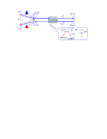
Figure 1: Proposed dynamical atom-cavity memory scheme. The cavity couples effectively to only one external incoming and outgoing mode, labelled here as $u_{0}^{in}$ and $u_{0}^{out}$ respectively. This implies an optimal pulse shape necessary for efficient imprinting and retrieval of the quantum information, as represented by the mode $a_{0}$, onto and from the atomic medium internal to the cavity. Storage is achieved through modulation of the atom-cavity coupling $g$ or detuning $\Delta$.

In this paper, we propose that these limitations may be overcome with the employment of a dynamical oscillator-cavity quantum memory. While useful in generation of squeezed and entangled states, most experimental quantum memories have not so far focused on intra-cavity interactionsstoring cavity1 ; storing cav 2 ; storecav3 ; theorycavity2 ; cavityqcomp ; cavpromise , apart from recent single-photon experimentsVuletic2007 ; Rempe2007 ; Vogel2008 . A limiting factor has been the lack of a full theoretical treatment of the interplay between the storage medium, the cavity and the incoming mode dynamics, together with their effect on memory performance.

Here, we bridge this gap by analyzing the memory dynamics of models of quantum memories, to calculate directly the memory response in the time domain. This allows further insight over previous treatments, which have been restricted by the assumption of slowly varying incoming signals in an adiabatic approximationtheory cavity ; theory cavity 3 ; lulinprl2000 ; scottkimble ; theorycavityDanpulse . Our theoretical approach is carried out with simple non-saturating linear oscillator models that are analytically soluble. This strategy can be applied to more general models, which behave as simple oscillators for low input signal intensities.

Our conclusion is that for quantum memories employing a coupled oscillator-cavity strategy, there is a critical coupling between the oscillator and cavity that gives an optimal temporal mode structure to allow for high efficiency and fidelity of input and output states. For low loss oscillator memories, this allows both high fidelity and long storage times in the cavity relative to the input pulse-width. The critical cavity coupling is closely related to the critical damping of a harmonic oscillator. We show that one can achieve the memory by either a modulation of the coupling or the detuning of the oscillator mode that stores the quantum state.

For a step-function gate the corresponding temporal mode has an asymmetric shape with duration of the order of the cavity ring-down time, which can be fast compared to the atomic decay time. In our treatment, the output mode is a time-reversed copy of the input. This time-reversal of an asymmetric mode could cause problems, for example, in local oscillator measurements or using cascaded devices. However, in a future paper, we show that the mode-shape can be further optimized with a time-dependent coupling, which leads to a fully time-symmetric mode in which both the input and output modes are identical.

Our results are applicable to any technologies employing cavity-like storage with a linear intra-cavity response. One example of this, as indicated above, would be the case of an ensemble of atoms with two or three-level transitions, as typically utilized in current experiments. Other possibilities include memories using superconducting cavities with Josephson junction qubit storagesolidstcircuits , and states encoded into positions of atomsscottkimble , molecules or even nano-oscillatorsVahala ; MarquardtCooling ; Harris2008 . The theoretical approach developed in this paper can also be extended to apply to spatial mode-structuresHak84 ; Drummond1981 , as will be analyzed elsewhere.

I Linear Memory

The quantum memory device we consider is that of a propagating single transverse-mode field $A^{in}(t)$ entering a cavity with an atomic or other oscillator medium (Fig. 1). Writing into the memory occurs up to a time $t=0$, during which time there is a nonzero interaction, between field and cavity, to allow the transfer of information. After a controllable storage time $T$, when the interaction is off, the interaction is switched on again, so the memory reads out into an outgoing quantum field $A^{out}(t)$ at $t>T$ (Fig. 2). The present paper focuses on fields with single transverse modes that are spatially mode-matched to the memory deviceDrummond1981 ; DruRay91 . We consider linear memories which are agnostic with regard to the quantum state or protocol, apart from a physical upper bound to the pulse energy.

I.1 Atomic example

There are many possible implementations in which a quantum system is coupled to an interferometer mode. To illustrate this, we first consider the classic caseHak84 ; Drummond1981 of a two-level near-resonant atomic medium, with a microscopic Hamiltonian of form:

$$\hat{H}_{af}=\sum_{j}\hat{H}_{j}\,,$$ (1)

where the Hamiltonian terms are given by:

$$\hat{H}_{1} = \hbar\sum_{k}\omega_{k}\hat{a}_{k}^{\dagger}\hat{a}_{k}$$

$$\hat{H}_{2} = \frac{\hbar}{2}\sum_{\mu}\omega_{\mu}(t)\hat{\sigma}_{\mu}^{z}$$

$$\hat{H}_{3} = \hat{H}^{a}+\hat{H}^{f}$$

$$\hat{H}_{4} = \hbar\sum_{k}\sum_{\mu}\left(g_{k}\left(t,\mathbf{r}_{\mu}\right)\hat{a}_{k}^{\dagger}\hat{\sigma}_{\mu}^{-}+H.c.\right)$$

$$\hat{H}_{5} = \hbar\sum_{\mu}\left(\hat{\Gamma}_{\mu}^{\sigma\dagger}\hat{\sigma}_{\mu}^{-}+\hat{\Gamma}_{\mu}^{\sigma}\hat{\sigma}_{\mu}^{+}+\hat{\Gamma}_{\mu}^{z}\hat{\sigma}_{\mu}^{z}\right)$$

$$\hat{H}_{6} = i\hbar\sum_{k}\left(\hat{\Gamma}_{k}^{a}\hat{a}_{k}^{\dagger}-\hat{\Gamma}_{k}^{a\dagger}\hat{a}_{k}\right)\,.$$ (2)

Here the rotating-wave and dipole approximations are employed, and the Hamiltonian terms have the interpretation as follows:

• $\hat{H}_{1}$ - paraxial mode free Hamiltonian

• $\hat{H}_{2}$ - atomic transition free Hamiltonian

• $\hat{H}_{3}$ - interferometer and atomic reservoir free Hamiltonians

• $\hat{H}_{4}$ - atom-field interaction Hamiltonian

• $\hat{H}_{5}$ - atom-reservoir interaction Hamiltonian

• $\hat{H}_{6}$ - field-reservoir interaction Hamiltonian

The frequencies $\omega_{k}$ are the mode-frequencies of the $k$-th interferometer modes, with annihilation operator $\hat{a}_{k}$. The sum over $k$ is restricted to a single polarization, under the assumption that only a single polarization of the cavity field is excited here, with momentum near $\mathbf{k}_{0}$ - which is the longitudinal photon momentum at the carrier wavelength.

The frequencies $\omega_{\mu}(t)$ are the transition frequencies of the $\mu$-th atomic transition. In general these may be time-dependent, for example, if an external magnetic field is used to create a time-varying Zeeman splitting. The corresponding operators are $\hat{\sigma}_{\mu}^{-}=\left|2\right\rangle_{\mu}\left\langle 1\right|_{\mu}$ and $\hat{\sigma}_{\mu}^{z}=\left|2\right\rangle_{\mu}\left\langle 2\right|_{\mu}-\left|1\right\rangle_{\mu}\left\langle 1\right|_{\mu}$. Similarly, the coupling term $g_{k}\left(t,\mathbf{r}_{\mu}\right)$ may be time and space-dependent, via the use of a time and space varying control field. In a pure two-level system, this coupling term would be expressed as:

$$g_{k}\left(t,\mathbf{r}_{\mu}\right)=g\left(t\right)u_{k}\left(\mathbf{r}_{\mu}\right)$$ (3)

Here $g\left(t\right)=\left[\mu^{2}\left(t\right)\omega_{c}/2\hbar\varepsilon_{0}\right]$ , where $\mu\left(t\right)$ is the electric dipole moment of the atomic transition. This can be made time-dependent in the case of forbidden transitions in even isotopes of alkaline earths, using a magnetic control fieldHollberg . As usual, $u_{k}\left(\mathbf{r}_{\mu}\right)e^{-i\mathbf{k}_{0}\cdot\mathbf{r}_{\mu}}$ is the mode function of a running wave with longitudinal momentum equal to $\mathbf{k}_{0}$ and a transverse mode structure of $u_{k}\left(\mathbf{r}_{\mu}\right)$, assumed not to depend on the longitudinal position in the simplest cases.

With a three-level atom and electromagnetic control field, the coupling term has a more complex behaviour that depends on the dynamics of a third level, which we have assumed can be eliminated if it has a far-off-resonant Raman coupling. The resulting coupling term has the structure:

$$g_{k}\left(t,\mathbf{r}_{\mu}\right)=g\left(t\right)\Omega\left(\mathbf{r}_{\mu}\right)u_{k}\left(\mathbf{r}_{\mu}\right)$$ (4)

A consequence of this structure of the coupling constant is that there may be two distinct spatial variations involved: one from the control field, and one from the stored quantum field. For simplicity, we will assume a spatially uniform control field intensity so that $\Omega\left(\mathbf{r}_{\mu}\right)=1$ in the following analysis, and we will absorb the phase variation of the control field into a single mode function $u\left(\mathbf{r}_{\mu}\right)$ with modulus $U_{\mu}$.

Generically, it is possible to divide up the atoms into equivalence classes with the same coupling constant modulus $U_{j}$ and transition frequency $\omega_{j}$. If the coupling constant and relevant field modes have radial symmetry, these correspond to distinct radial shells.

This creates a set of inequivalent atomic spin operators, defined as:

$$\hat{J}_{j}^{+} = \sum_{\mu\in s(j)}\hat{\sigma}_{\mu}^{+}u^{*}\left(\mathbf{r}_{\mu}\right)/U_{j}$$

$$\hat{J}_{j}^{-} = \sum_{\mu\in s(j)}\hat{\sigma}_{\mu}^{-}u_{k}\left(\mathbf{r}_{\mu}\right)/U_{j}$$

$$\hat{J}_{j}^{z} = \sum_{\mu\in s(j)}\hat{\sigma}_{\mu}^{z}$$ (5)

Initially ignoring (initially) the effects of atomic reservoirs and losses, which should be small in an atomic system intended for use as a quantum memory, the resulting Heisenberg picture field and atomic equations in the rotating-wave and paraxial approximations are as follows:

$$\frac{\partial}{\partial\,t}\hat{a} = -\left(i\omega_{0}+\kappa\right)\hat{a}-i\sum_{j}g_{j}\left(t\right)\hat{J}_{{\bf j}}^{-}+\hat{\Gamma}_{k}$$

$$\frac{\partial}{\partial\,t}\hat{J}_{j}^{-} = -i\omega_{j}\hat{J}_{j}^{-}+ig_{j}^{*}\left(t\right)\hat{a}\left(t\right)\hat{J}_{{\bf j}}^{z}$$

$$\frac{\partial}{\partial\,t}\hat{J}_{j}^{z} = 2\left[ig_{j}\left(t\right)\hat{a}^{\dagger}\hat{J}_{j}^{-}+H.c.\right]$$ (6)

Here $g_{j}\left(t\right)=g\left(t\right)U_{j}$, and there are also corresponding equations for conjugate fields. This assumes that the mode function does not vary rapidly over the location of the grouped atoms.

We note here that in general there may be many distinct transverse electromagnetic mode functions $u_{k}$ that are able to couple to the atoms. In addition, the cavity loss is at a rate $\kappa_{k}$ due to coupling to the cavity output fields, while $\hat{\Gamma}_{k}$ is the quantum operator for the input and output fields with different transverse mode indices $k$. According to standard input-output theorycollgard84 ; gardcoll85 ,

$$\hat{\Gamma}_{k}=\sqrt{T_{o}/\tau_{r}}\left(\widehat{A}_{k,in}-\widehat{A}_{k,out}\right)\,\,,$$ (7)

where $\widehat{A}_{k,in}$ is the input photon field and $\widehat{A}_{k,out}$ is the output field, while $T_{o}$ is the mirror transmissivity of the output coupler, and $\tau_{r}$ is the cavity round-trip time.

In this paper we will only consider the case of a single-mode interferometer interacting with a non-saturated homogeneous medium, so that $\hat{J}_{j}^{z}\approx-N_{j}$. We can introduce an effective harmonic oscillator operator of:

$$\widehat{b}=\frac{1}{g(t)}\sum_{j}g_{j}\left(t\right)\hat{J}_{{\bf j}}^{-}\,,$$ (8)

where $g=\sqrt{\sum_{j}N_{j}\left|g_{0,j}^{2}\left(t\right)\right|}$. We also assume that the medium has a single resonance at $\omega_{j}=\omega$, which means that there is no inhomogeneous or Doppler broadening. This would require cooling and possibly trapping in an optical lattice to eliminate atomic motion. The corresponding Heisenberg equations are:

$$\frac{\partial}{\partial\,t}\hat{a} = -\left[\kappa+i\omega_{0}\right]\hat{a}-ig\left(t\right)\hat{b}+\hat{\Gamma}$$

$$\frac{\partial}{\partial\,t}\widehat{b} = -i\omega\hat{b}-ig\left(t\right)\hat{a}_{{\bf k}}\left(t\right)\,.$$ (9)

In a rotating frame resonant with the input carrier frequency of the quantum signal $\omega_{L}$, this leads to the following effective Hamiltonian:

$$H=\hbar\delta\widehat{a}^{\dagger}\widehat{a}+\hbar\Delta\widehat{b}^{\dagger}\widehat{b}+\hbar g(t)(\widehat{b}^{\dagger}\widehat{a}+\widehat{a}^{\dagger}\widehat{b})\,.$$ (10)

where $\delta=\omega_{0}-\omega_{L}$, $\Delta=\omega-\omega_{L}$. This one-photon detuning $\Delta$ is replaced by the two photon detuning in the case of a Raman-type interaction.

I.2 Nanomechanical oscillators

Similar results are obtained for the effective Hamiltonian of mechanical oscillators - like an atomic position or nanomechanical oscillator - in a cavityWalls ; scottkimble ; Harris2008 . In this case the position oscillation has a frequency that is physically analogous to the separation of the two lower levels in a three-level atomic model. A control field is needed to create a Raman transition between the oscillator levels. This type of situation is studied theoretically as a means of laser cooling nanomechanical oscillators, which has been recently demonstrated experimentallyVahala .

To derive this relationship, we start with a microscopic Hamiltonian for the radiation field inside an interferometer coupled to a nano-mechanical oscillator, interacting via the dielectric energy of the coupled systemDrummondQuant . This gives a Hamiltonian of form:

$$\hat{H}_{nano}=\sum_{j}\hat{H}_{j}\,,$$ (11)

where the Hamiltonian terms are given by:

$$\hat{H}_{1} = \hbar\sum_{k}\omega_{k}\hat{a}_{k}^{\dagger}\hat{a}_{k}$$

$$\hat{H}_{2} = \hbar\sum_{\mu}\omega_{j}^{m}\hat{b}_{j}^{\dagger}\hat{b}_{j}$$

$$\hat{H}_{3} = \hat{H}^{a}+\hat{H}^{b}$$

$$\hat{H}_{4} = \hbar\int d^{3}\mathbf{r}\left(\frac{1}{\varepsilon(\mathbf{r})}-\frac{1}{\varepsilon_{0}}\right)\left|\hat{\mathbf{D}}\left(\mathbf{r}\right)\right|^{2}$$

$$\hat{H}_{5} = i\hbar\sum_{j}\left(\hat{\Gamma}_{j}^{b}\hat{b}_{j}^{\dagger}-\hat{\Gamma}_{j}^{b\dagger}\hat{b}_{j}\right)\,$$

$$\hat{H}_{6} = i\hbar\sum_{k}\left(\hat{\Gamma}_{k}^{a}\hat{a}_{k}^{\dagger}-\hat{\Gamma}_{k}^{a\dagger}\hat{a}_{k}\right)\,.$$ (12)

Here the Hamiltonian terms have the interpretation:

• $\hat{H}_{1}$ - paraxial mode free Hamiltonian

• $\hat{H}_{2}$ - nano-mechanical oscillator free Hamiltonian

• $\hat{H}_{3}$ - interferometer and oscillator reservoir free Hamiltonians

• $\hat{H}_{4}$ - interaction energy of the nano-oscillator dielectric in an external field

• $\hat{H}_{5}$ - oscillator-reservoir interaction Hamiltonian

• $\hat{H}_{6}$ - field-reservoir interaction Hamiltonian

The frequencies $\omega_{k}$ are the mode-frequencies of the $k$-th interferometer modes, with annihilation operator $\hat{a}_{k}$, as previously. The frequency $\omega_{j}^{m}$ is the $j-$th resonant mode frequency of the nano-mechanical oscillator. The field $\hat{\mathbf{D}}\left(\mathbf{r}\right)$is the electromagnetic displacement field;

$$\hat{\mathbf{D}}\left(\mathbf{r}\right)=\sum_{k}\left[\frac{\hbar\omega_{k}\varepsilon\left(\mathbf{r}\right)}{2}\right]\left(u_{k}\left(\mathbf{r}\right)\hat{a}_{k}+H.c.\right)$$ (13)

which is the relevant canonical field variable. We note that for a standing wave interferometer, with only a single mode of the resonator and nano-mechanical oscillator, this will reduce to the standard quantum model of a nano-oscillator as a movable mirror or dielectric inside a cavityWalls :

$$H=\hbar\delta\widehat{a}^{\dagger}\widehat{a}+\hbar\omega^{m}\widehat{b}^{\dagger}\widehat{b}+\hbar g\widehat{a}^{\dagger}\widehat{a}(\widehat{b}^{\dagger}+\widehat{b})\,.$$ (14)

Here, $\delta=\omega_{0}-\omega_{L}$, and $\omega^{m}$ is the resonant frequency of the nanomechanical oscillator.

Since we wish to eliminate the effects of direct radiation pressure on the oscilator dielectric, we treat a running-wave in which the field modes by themselves are not coupled to the oscillator motion, to lowest order. Next, suppose there is an additional counterpropagating control field $\Omega(t)e^{i\omega_{c}t}$ incident on the oscillator. This additional field is able to interfere either constructively or destructively with the intracavity field, at the mirror location. Let $\omega_{c}=\omega_{0}-\omega$, so the control field is red-detuned with respect to the Fabry-Perot resonance, which is precisely the condition required for sideband cooling of a nano-mechanical oscillator. We will also assume, for simplicity, that the experimental goal of cooling to the oscillator ground-state is achieved, which means that the heating rate of the oscillator due to its thermal reservoirs is sufficiently small.

This leads to the following effective Hamiltonian, in which non-resonant terms are neglected:

$$H = \hbar\delta\widehat{a}^{\dagger}\widehat{a}+\hbar\Delta\widehat{b}^{\dagger}\widehat{b}+$$ (15)

$$+ \hbar g(\Omega^{*}(t)\widehat{a}\widehat{b}^{\dagger}+\Omega(t)\widehat{a}^{\dagger}\widehat{b})$$

We see that, for a real control field with $g(t)=g\Omega(t)$, this expression is identical to the one derived for the case of a weakly excited atomic resonance.

I.3 Input/output mode expansions

As is common in scattering theory, we can define input and output modes corresponding to two distinct Hilbert spaces for the asymptotic past and future of the memory. We limit ourselves to treating a single transverse mode $A_{0}^{in}(t)$ for simplicity. A complete mode expansion into longitudinal modes of the incoming external field for past times $t<0$ is

$$\widehat{A}_{0}^{in}(t)=\sum_{n}\widehat{a}_{n}^{in}u_{n}^{in}(t)\,,$$ (16)

where $\widehat{A}_{0}^{in}$ is a boson input field such that $\left[\widehat{A}_{0}^{in}(t),\widehat{A}_{0}^{in\dagger}(t^{\prime})\right]=\delta(t-t^{\prime})$. Here the $a_{n}^{in}$ are bosonic mode operators and $u_{n}^{in}(t)$ the mode functions, whose expectation values determine the incoming pulse shape. Similarly, the operator $\widehat{A}_{0}^{out}(t)$ is the quantum operator for the output field. A complete mode expansion for the outgoing external field after a memory storage time $T$ is an expansion over future times ($t>T$):

$$\widehat{A}_{0}^{out}(t)=\sum_{n}\widehat{a}_{n}^{out}u_{n}^{in}(t)\,,$$ (17)

where the $\widehat{a}_{n}^{out}$are also boson annihilation operators, and the $u_{n}^{out}(t)$ the output mode functions. We focus on the simplest possible case of single longitudinal mode storage devices, which are designed to accurately write into memory, store then read out information for one input and one output bosonic mode. The single-mode input and output operators of the states to be “remembered” will be labelled $\widehat{a}_{n}^{in}$ and $\widehat{a}_{n}^{out}$ . To simply the typography, we will omit the caret on single mode operators $a$, $b$ and fields $A$, $B$ in the remaining sections.

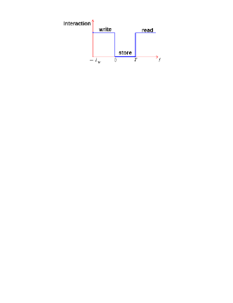
Figure 2: Memory involves three stages: writing, reading and storing. The interaction is turned on, then off, then on, in a controllable way.

II Memory Fidelity

It is crucial to determine the level of memory performance and accuracy at which one can convincingly claim a “quantum memory”. A standard figure of merit for memory performance is that of the average fidelity $\bar{F}$ between input and output states, as defined over a predetermined set of input states. Here the output state is a density matrix $\hat{\rho}_{out}$, which is obtained on tracing the output state over the input modes and loss reservoirs:

$$\hat{\rho}_{out} = Tr_{r}\left[|\Psi_{out}\rangle\langle\Psi_{out}|\right]$$ (18)

$$= Tr_{r}\left[\hat{U}|\Psi_{in}\rangle\langle\Psi_{in}|\hat{U}^{-1}\right]\,.$$

We will be considering pure state inputs, in which case the average fidelity is defined as:

$$\bar{F}=\int P(\Psi_{in})\langle\Psi_{in}|\hat{\rho}_{out}(\Psi_{in})|\Psi_{in}\rangle d\mu(\Psi_{in})$$ (19)

Here $P(\Psi_{in})$ is the probability of using a given state $\Psi_{in}$, while $\hat{\rho}_{out}(\Psi_{in})$ is the output density matrix conditioned on input of $\Psi_{in}$, and $d\mu(\Psi_{in})$ is the integration measure used over the set of input states.

The average fidelity obtained must be compared with the best average fidelity possible using a ‘classical’ measure, store and prepare strategy, in order to claim that one has a quantum memory. There is no known limit to which quantum states may be feasibly prepared, nor on what observables can be measured, except that the commutators of quantum mechanics prevent simultaneous, precise measurement of non-commuting variables. This means that the set of inputs used is important in establishing fidelity bounds. For example, if the input states are orthogonal - like the number states - then the classical fidelity bound is unity. All the number states can in principle be measured using a perfect photo-detector, the corresponding number recorded and stored, followed by regeneration of the original number state with perfect fidelity.

This means that superpositions must be an integral part of the input alphabet of quantum states. An important issue is that the relative phase of superpositions must be recalled in a quantum memory device. Thus, the fidelity can not be measured in the same way as the photon counting efficiency: a memory that generates outputs with random phases will have a high photon-counting efficiency, but a low quantum fidelity. This is because the fidelity measure is phase-sensitive, which is essential for a quantum memory. To experimentally characterize a quantum memory it is therefore necessary to measure input and output states interferometrically. Measuring the energy efficiency alone cannot rule out memory phase errors caused, for example, by timing jitter in the control signals.

II.1 Linear memory

In this paper, we treat linear memory models, with all reservoirs in the vacuum state, and with no excess phase noise. This type of memory has the useful property that it is able, ideally, to preserve any input state with a subsequent time-delayed read-out.

In quantum mechanics, a given initial state $|\Psi_{in}\rangle$ in the Schroedinger picture is transformed to a final state by making a unitary transformation on the input Hilbert space:

$$|\Psi_{out}\rangle=\hat{U}|\Psi_{in}\rangle\,.$$ (20)

In greater detail, we can divide the Hilbert space into the input space, output space, and reservoir space consisting of all other degrees of freedom. We assume that initially the input space has a factorized state :

$$|\Psi_{in}\rangle=|\psi_{0}\rangle_{in}|0\rangle_{out}|0\rangle_{r}$$ (21)

The purpose of a quantum memory is to transform this input state into an output state at a later time, with the structure:

$$|\Psi_{out}\rangle=|0\rangle_{in}|\psi_{0}\rangle_{out}|0\rangle_{r}$$ (22)

It is convenient to describe the input in terms of a function of input mode creation operators $a_{0}^{\dagger}$ defined at $t=-\infty$, so that:

$$|\psi_{0}\rangle=f\left(a_{0}^{\dagger}\right)|0\rangle_{in}$$ (23)

We will find in the next sections that in the Heisenberg picture, the overall effect of either losses or mode mis-matching is identical to a (time-delayed) beam-splitter with transmission efficiency $\eta_{M}$, so that the memory output state is:

$$|\Psi_{out}\rangle=|0\rangle_{in}f\left(a_{0}^{\dagger}(\infty)\right)|0\rangle_{out}|0\rangle_{r}$$ (24)

where:

$$a_{0}(\infty) = \sqrt{\eta_{M}}a_{0}+\sqrt{1-\eta_{M}}a_{0}^{r}\,.$$ (25)

Here $a_{0}$ is now understood to act on the output vacuum state, and $a_{0}^{r}$ is a bosonic operator which only acts on the zero-temperature reservoir, so that $\langle a_{0}^{r\dagger}a_{0}^{r}\rangle_{r}=0$.

Ideal performance is obtained when retrieval efficiency $\eta_{M}=1$, so that the input and output mode operators are identical, apart from the technical issue that they are defined on different Hilbert spaces. In practice, loss and noise will be introduced at all three stages of a quantum memory: not all information can be retrieved, since $\sqrt{\eta_{M}}<1$.

II.2 Coherent state memories

The most common set of input states considered to date are coherent states, which have already proved useful to quantum applications such as teleportationfurteleport and quantum state transfer from light onto atomsJulsgaard . If we consider our input set as the set of coherent states with a Gaussian distribution $P(\alpha)=1/(\overline{n}\pi)e^{-|\alpha|^{2}/\overline{n}}$, and mean photon number $\overline{n}$, the fidelity average measure $\overline{F}$ is

$$\bar{F}_{\bar{n}}^{g}=\int P(\alpha)\langle\alpha|\hat{\rho}_{out}(\alpha)|\alpha\rangle d^{2}\alpha\,,$$ (26)

where $\hat{\rho}_{out}(\alpha)$ is the output state for the coherent input state $|\alpha\rangle$.

The results of Hammerer et alHammerer and Braunstein et albraun show that for any classical channel, the average fidelity is constrained by

$$\bar{F}_{\bar{n}}^{g}\leq(1+\overline{n})/(2\overline{n}+1)\,.$$ (27)

Thus, the result $\bar{F}_{\bar{n}}^{g}>(1+\overline{n})/(2\overline{n}+1)$ serves as a benchmark for the claim of a quantum memory of coherent states.

We calculate $\bar{F}_{\bar{n}}^{c}$ for our beam-splitter solution Eq. (25). In this solution, the output is $\hat{\rho}_{out}(\alpha)=|\sqrt{\eta_{M}}\alpha\rangle\langle\sqrt{\eta_{M}}\alpha|$. Simple calculation gives

$$\bar{F}_{\bar{n}}^{c}=\frac{1}{1+\overline{n}(1-\sqrt{\eta_{M}})^{2}}\,.$$ (28)

The condition for quantum memory (so that (27) is violated) is thus satisfied for efficiencies

$$\sqrt{\eta_{M}}>1-\sqrt{\frac{1}{\overline{n}+1}}\,.$$ (29)

We note that for $\overline{n}\geq 20,$ the bound follows an almost flat line relation to $\bar{n}$, which is the well known flat distribution for which fidelity $\bar{F}_{\infty}^{c}>0.5$ is required for a quantum memoryHammerer ; Julsgaard ; furteleport . These fidelities correspond in the beam splitter memory to quite high efficiencies, so for $\overline{n}=20$, quantum memory is achieved for $\sqrt{\eta_{M}}>0.78$. For $\overline{n}$ small, say $\overline{n}=1$, which requires fidelity $\bar{F}_{1}^{c}>2/3,$ we note that quite low efficiencies ($\sqrt{\eta_{M}}>0.293$) are enough for a claim of a quantum memory (Fig. 3).

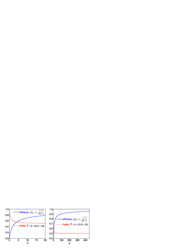
Figure 3: Fidelity $\bar{F}_{\bar{n}}^{c}$ (dashed) and corresponding beam splitter efficiency $\sqrt{\eta_{M}}$ (solid) required for quantum memory as a function of $\bar{n}$ for coherent input states. High $\bar{n}$ will require a high efficiency $\eta_{M}$, for the claim of a quantum memory, whereas for low $\bar{n}$ , quantum memory is achievable for lower efficiencies. Horizontal lines indicate the respective classical bounds.

II.3 Arbitrary state memories

An ideal quantum memory must do more than just store coherent states. For many quantum information applications, the quantum states that must be stored may be in a larger class of possible quantum inputs. Recent experiments and theory have investigated other possibilities, like squeezed statessqbenchmark ; Appel ; honda . The most general case is a completely arbitrary quantum input state. However, it is essential to bound the input energy in some way. Otherwise, the averages are dominated by inputs of infinitely large energy, that no physical memory could possibly store without giving rise to a black hole.

Here we define the input state as any possible state with a maximum photon number less than $n_{m}$. This corresponds to an arbitrary state $\left|\vec{\Psi}\right\rangle$ of $n_{m}$ levels, where:

$$\left|\vec{\Psi^{in}}\right\rangle=\sum_{n=0}^{n_{m}-1}\Psi_{n}\left|n\right\rangle\,.$$ (30)

so that the highest photon number is $n=n_{m}-1$. The fidelity average $\overline{F}_{n_{m}}$ is then the average fidelity over all possible coefficients $\vec{\Psi}$, satisfying the constraint that $\left|\vec{\Psi}\right|=1$ , i.e:

$$\bar{F}_{n_{m}}=\frac{\int\delta(\left|\vec{\Psi}\right|-1)\langle\vec{\Psi}|\hat{\rho}_{out}(\vec{\Psi})|\vec{\Psi}\rangle d^{2n_{m}}\vec{\Psi}}{\int\delta(\left|\vec{\Psi}\right|-1)d^{2n_{m}}\vec{\Psi}}\,,$$ (31)

where $\hat{\rho}_{out}(\vec{\Psi})$ is the output reduced density matrix for the arbitrary bounded input state $|\vec{\Psi}\rangle$, after tracing over any reservoirs coupled to the memory.

To determine the classical fidelity limit in this case, we recall that there is a known fidelity limit for (imperfect) cloning of an arbitrary $n_{m}$ level state, to produce an infinitely large number of copies. This limit is that classical clone :

$$\bar{F}_{n_{m}}\leq\frac{2}{n_{m}+1}\,.$$ (32)

Since a classical memory can clearly generate any number of copies of a quantum state, this result shows that for any classical memory with an arbitrary input of bounded maximum photon number, the average fidelity is constrained by the one-to-many cloning limit.

We now calculate $\bar{F}_{n_{m}}$ for our beam-splitter solution Eq. (25). The total input state, including a reservoir labelled $r$ and assumed to be a vacuum state, is:

$$\left|\Psi_{T}^{in}\right\rangle=\sum_{n=0}^{n_{m}-1}\frac{\Psi_{n}}{\sqrt{n!}}\hat{a}^{\dagger n}|\mathbf{0}\rangle\,.$$ (33)

Here $\Psi_{n}$ is the probability amplitude for the $|n\rangle$ input state. The output state is therefore:

$$\left|\Psi^{out}\right\rangle = \hat{U}\left|\Psi_{T}^{in}\right\rangle$$

$$= \sum_{n=0}^{n_{m}-1}\frac{\Psi_{n}}{\sqrt{n!}}\left[\hat{a}^{out\dagger}\right]^{n}|\mathbf{0}\rangle\,$$

$$= \sum_{n=0}^{n_{m}-1}\frac{\Psi_{n}}{\sqrt{n!}}\left[\sqrt{\eta_{M}}a_{0}^{in\dagger}+\sqrt{1-\eta_{M}}a_{0}^{r\dagger}\right]^{n}|\mathbf{0}\rangle\,.$$

We can now calculate the fidelity in the case of $n_{m}=2$ and $n_{m}=3$, which allows for arbitrary states with up to $1$ and $2$ photons respectively. Since the reservoir modes are not the input to the memory, we trace over the mode $r$, to obtain the predicted memory fidelities

$$\overline{F}_{2} = \frac{\eta_{M}+2\sqrt{\eta_{M}}+3}{6}$$

$$\overline{F}_{3} = \frac{\eta_{M}^{2}+2\eta_{M}\sqrt{\eta_{M}}+3\eta_{M}+2\sqrt{\eta_{M}}+4}{12}\,.$$ (35)

for 2 and 3-dimensional (up to $1$ and $2$ photon number) input states respectively. These results are graphed below, in Fig. 4.

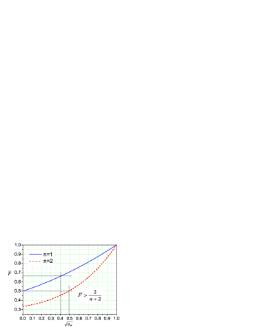
Figure 4: Average fidelity vs beam splitter efficiency of a quantum memory for arbitrary input states with up to $n=1$ (solid line) and $n=2$ (dashed line) photons.

It is straightforward to prove, using SU(n) symmetry, that in the limit of zero efficiency the quantum memory will have an average fidelity of $\overline{F}_{n_{m}}=1/n_{m}$ . This is always less than the fidelity achievable by a classical “measure and regenerate” strategy. In general, the best classical average fidelity decreases as the number of possible quantum levels increases. This is easily understandable: a single measurement gives very little information about the coherent superpositions that may exist in a quantum state with many levels. For this reason, an arbitrary quantum state fidelity measure gives a much better indication of the power of a quantum memory than a measure constrained to a single set of states like the coherent states. This gives a strong motivation for more general experimental tests of quantum memory performance.

III Q-switched memory dynamics: mode matching

In the previous sections, we calculated the fidelity where the relation between the input and output states is describable by the beam splitter solution Eq. (25). Now, we show under which conditions this solution is predicted. To understand the role of mode-matching, we examine in this section the simple model of an empty Q-switched cavity.

We consider first a simplistic quantum memory model of an empty Q-switched cavity, tuned to frequency $\omega_{0}=\omega_{L}+\delta$. In practice, long storage times are not readily achievable without a separate oscillator such as an atom medium for storage. However, we analyse this model first to develop an understanding of the dynamics of the three stages of memory process: writing, storage and reading. The corresponding effective internal Hamiltonian is:

$$\widehat{H}=\hbar\delta a^{\dagger}a\,.$$ (36)

The cavity is partially transmitting, with variable cavity decay rate $\kappa(t)$, allowing a coupling between the cavity mode $a$ and a pulsed input field $a_{in}(t)$. For a cavity whose only loss is through one mirror acting as an input/output coupler, the dynamical Heisenberg equation linking input and cavity mode operators iscollgard84 ; gardcoll85

$$\dot{a}=-\left[i\delta(t)+\kappa(t)\right]a+\sqrt{2\kappa(t)}A^{in}(t)\,.$$ (37)

The writing stage begins at $-t_{w}$ (Fig. 2) and is of duration up to $t=0$. Defining a time-evolution function:

$$T_{\kappa}(t,t^{\prime})=\exp\left[-\int_{t^{\prime}}^{t}\left[i\delta(\tau)+\kappa(\tau)\right]d\tau\right]\,,$$ (38)

the interaction given by Eq. (37) has the general solution

$$a(t) = T_{\kappa}(t,-t_{w})a(-t_{w})+$$ (39)

$$+ \int_{\tau=-t_{w}}^{t}T_{\kappa}(t,\tau)\sqrt{2\kappa(\tau)}A^{in}(\tau)d\tau\,.$$

The purpose of the memory is to read in the field at $t<0$, and then output selected information after a memory time $T$. We therefore introduce a model decay rate with Q-switching between a large value $\kappa$ and a small value $\kappa_{S}$, at zero detuning:

$$\kappa(t) = \kappa\,\,\,[t<0]$$

$$\kappa(t) = \kappa_{S}\,\,\,[0<t<T]$$

$$\kappa(t) = \kappa\,\,\,[t>T]\,.$$ (40)

We note here as a practical issue that all cavities have excess loss and noise over and above that given just by considering input/output couplers. This may be unimportant during the input/output stages, when $\kappa(t)$ is large. However, it is certainly significant when $\kappa(t)$ is small. For this reason, $\kappa_{S}$ and the corresponding vacuum reservoir term must include all losses during the storage time, including loss in the dielectric coatings and diffraction losses. Additional phase-noise and corresponding phase-relaxation terms due to acoustic noise are ignored for simplicity.

We note our model quantum memory has a time-reversal symmetry around $t=T/2$, since $\kappa(t)=\kappa(T-t)$. This is not essential, since one could easily choose $\kappa(t>T)\neq\kappa(t<0)$ . However, this feature - which is also found in some other memory proposals - provides a useful insight into design of a quantum memory, and the mode-functions that are coupled into and out of the memory. Here, of course, time-reversal implies reversing the propagation direction of all fields, including the input and output fields. A typical input-output relation with some residual loss during the storage time is shown in Fig. 5. This is obtained from a numerical solution of Eq. (37) in a P-representationPrep , which transforms the operator equations into c-number equations. In this case, the input state of the field is assumed to be a coherent state. The calculated solution clearly displays the time-reversal. We note that the calculation can be extended to an arbitrary initial state using the positive P-representation methodposP .

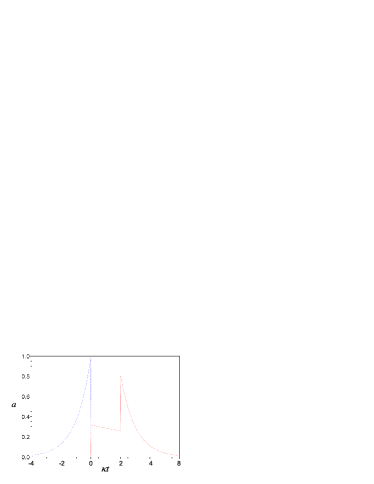
Figure 5: Q-switched cavity input (dashed blue line) and output (solid red line) amplitudes with $\kappa=1$, $\kappa_{S}=0.1$, $T=2.0$. Input mode shape is mode matched to the time-reversed cavity decay.

To explain the operation of the Q-switched quantum memory more clearly, we seek analytical solutions, and now expand the incoming and outgoing field operators into past-time ($t<0$) and future time ($t>T$) modes. This allows us to easily distinguish what is stored in the memory in the past from what is read out, in the future.

III.1 Writing: past-time modes

Our model gives for the stored cavity mode solution, when the cavity coupling is switched to a small value for storage:

$$a(0)=a_{0}^{in}\equiv\sqrt{2\kappa}\int_{-\infty}^{0}e^{\kappa\tau}A^{in}(\tau)d\tau\,.$$ (41)

Where we have considered $\delta=0$ for simplicity, which means that the cavity is resonant with the field carrier frequency. We have allowed the writing time $t_{w}$ to be infinite, in practice of duration much longer than pulse durations and cavity lifetimes, so as to erase information associated with the initial cavity solution.

We note the operator $A^{in}(t)$ is the quantum operator for the input field, but the coupling to the cavity is such that only a certain mode of this incoming field is effectively coupled. We choose our input mode expansion to be:

$$u_{n}(t)=\sqrt{2\kappa}e^{\kappa t}L_{n}(-2\kappa t)\Theta(-t)\,,$$ (42)

which are modified Laguerre polynomials. Since the Laguerre polynomials are a complete set, any incoming waveform that vanishes as $t\rightarrow-\infty$ can be represented as a linear combination of Laguerre functions. Introducing $z=-2\kappa t$, these have orthogonality relations of:

$$\int_{-\infty}^{0}u_{n}^{in}(t)u_{m}^{in*}(t)dt = \int_{0}^{\infty}e^{-2z}L_{n}(z)L_{m}(z)dz$$ (43)

$$= \delta_{mn}\,.$$

In this expansion, $u_{n}(t)$ are orthogonal mode functions on the space of past times, prior to switching on the memory at $t=0$, so that:

$$a_{n}^{in}=\int_{-\infty}^{0}A^{in}(t)u_{n}^{in*}(t)dt\,.$$ (44)

Thus, using the field commutators we obtain the following bosonic commutators for $a^{in}$:

$$\left[a_{n}^{in},a_{m}^{in\dagger}\right] = \int_{-\infty}^{0}\int_{-\infty}^{0}u_{n}^{in*}(t)u_{m}^{in}(t^{\prime})\delta(t-t^{\prime})dtdt^{\prime}$$ (45)

$$= \int_{-\infty}^{0}u_{n}^{in*}(t)u_{m}^{in}(t)dt$$

$$= \delta_{nm}\,.$$

Due to the orthogonality of the Laguerre functions only the $u_{0}(t)$ term will give a nonzero contribution to $a(0)$. To gain maximum efficiency of the memory, the experimentalist must therefore construct the incoming pulse shape to match this mode, so that $<a_{n}^{in}>=\delta_{0n}$. With this choice, when evaluating expectation values we can effectively simplify to a single input mode:

$$A^{in}(t)=u_{0}^{in}(t)a_{0}^{in}=\sqrt{2\kappa}e^{\kappa t}a_{0}^{in}\,.$$ (46)

We note that this saw-tooth type mode structure is time-asymmetric (see Fig. 5), which is not ideal in terms of mode matching to the typical Gaussian pulses produced by mode-locked lasers. Improved matching to symmetric pulses could be realized through more careful shaping of the cavity coupling in time, ie, making $\kappa(t)$ a prescribed shape.

We also stress that this cavity-based memory is a strictly mono-mode memory, from a temporal point of view. One temporal mode only is stored, the others being reflected. No bipartite (or n-partite) states composed of two or more temporal modes $u_{i}(t)$ can thus be stored. This device can however be used as a mode-converter to manipulate temporal multi-mode quantum states.

III.2 Storage period

In the simplest model, in which no medium is present and cavity losses are assumed zero, the value $a(0)$ is stored with maximum efficiency in the cavity for a duration $T$, so that

$$a(T)=a(0)\,.$$ (47)

More generally, there is a residual storage loss $\kappa_{S}$ at this stage. The dynamical Eq. (37) applies again, but this time as we have no pulsed input, the input $A^{in}(\tau)$ represents only the incoming vacuum field. To make a clear distinction between the two inputs, we will denote $A^{in}(t)\equiv A_{v}^{in}(t)$ where $t>T$, so that:

$$a(T)=e^{-\kappa_{S}T}a(0)+\sqrt{2\kappa_{S}}\int_{\tau=o}^{T}e^{\kappa_{S}(\tau-T)}A_{v}^{in}(\tau)d\tau\,.$$ (48)

When there are excess losses in addition to output coupler loss, $A_{v}^{in}(\tau)$ must include all the relevant loss reservoirs associated with $\kappa_{S}$ . Although we do not consider this in detail, there can also be additional noise sources which will degrade the stored quantum information. These include thermal noise if the signal is at relatively low frequency, as in microwave experiments, and additional phase noise from acoustic noise or $1/f$ noise in the mirrors and dielectrics. Phase-noise can become very significant in the limit of long storage times, and must be considered when storage fidelity is measured.

III.3 Reading: future-time modes

At time $T$, the output stage commences, and the cavity is switched back to a large $\kappa$, to allow transmission, or reading, of the remembered signal outside the cavity. The solution is

$$a(t)=e^{-\kappa(t-T)}a(T)+\sqrt{2\kappa}\int_{T}^{t}e^{\kappa(\tau-t)}A_{v}^{in}(\tau)d\tau\,.$$ (49)

We focus on the output field transmitted through the cavity, given bycollgard84 ; gardcoll85

$$A^{out}=\sqrt{2\kappa}a-A_{v}^{in}\,.$$ (50)

Making use of the time-reversal symmetry of our model, we will choose the output modes to be the time-reversed input modes, so that

$$u_{n}^{out}(t) = u_{n}^{in*}(T-t)$$ (51)

$$= \sqrt{2\kappa}e^{-\kappa(t-T)}L_{n}(2\kappa(t-T))\,.$$

Introducing $z=2\kappa(t-T)$, these have orthogonality relations in future time, of:

$$\int_{T}^{\infty}u_{n}^{out}(t)u_{m}^{out*}(t)dt = \int_{0}^{\infty}e^{-z}L_{n}(z)L_{m}(z)dz$$ (52)

$$= \delta_{mn}\,.$$

At this point, we note that maximum efficiency of retrieval is achieved if we temporally match the output with the input in the following way. We define the filtered output field operator as:

$$a_{0}^{out} \equiv \int_{T}^{\infty}u_{0}^{*}(t)A^{out}(t)dt\,$$ (53)

$$= \sqrt{2\kappa}\int_{T}^{\infty}e^{-\kappa(t-T)}A^{out}(t)dt\,.$$

We find

$$a_{0}^{out} = \sqrt{2\kappa}\int_{T}^{\infty}e^{-\kappa(t-T)}A^{out}(t)dt$$ (54)

$$= \sqrt{2\kappa}\int_{T}^{\infty}e^{-\kappa(t-T)}(\sqrt{2\kappa}a(t)-A_{v}^{in}(t))dt$$

$$= 2\kappa\int_{T}^{\infty}e^{-2\kappa(t-T)}a(T)dt$$

$$-2\kappa\sqrt{2\kappa}\int_{T}^{\infty}e^{-\kappa(t-T)}dt\int_{T}^{t}e^{\kappa(\tau-t)}A_{v}^{in}(\tau)d\tau$$

$$+\sqrt{2\kappa}\int_{T}^{\infty}e^{-\kappa(t-T)}A_{v}^{in}(t)dt$$

$$= a(T)\,.$$

In the ideal case with $\kappa_{S}=0$, we know that $a(T)=a(0)=a_{0}^{in}$, so we retrieve the signal $a_{0}^{in}$, while all information related to unwanted vacuum inputs at future times, $A_{v}^{in}$, is completely absent from the filtered output. The explanation of this desirable behaviour is rather simple. After $t=T$, the cavity is perfectly matched as an absorber of incoming vacuum modes to the future-time $u_{0}$ mode. As a result, the cavity now absorbs all the incoming vacuum field radiation in the incoming $n=0$ future-time mode, while simultaneously emitting the stored information in an outgoing $n=0$ future-time mode. In summary, while the modes with $n>0$ are simply reflected, the stored $n=0$ mode changes places with an incoming $n=0$ vacuum mode.

Thus, an incoming past-time $n=0$ mode is time-delayed by the memory time $T$, then re-emitted into an outgoing future-time $n=0$ mode. This is readable without losses (in the ideal case) using a temporal mode filter. We note that the pulse-shape of the output mode is time-reversed with respect to the input mode.

In our model of an empty Q-switched cavity with perfect temporal mode-matching and loss occurring during storage, the storage cannot be ideal. The presence of losses means not all information can be retrieved due to the residual loss $\kappa_{S}$ from the cavity over the storage time of duration $T$. This means that $a(T)\neq a(0)$. Instead

$$a(T) = e^{-\kappa_{S}T}a(0)+\sqrt{2\kappa_{0}}\int_{0}^{T}e^{\kappa_{S}(t-T)}A_{v}^{in}(t)dt$$ (55)

$$= \sqrt{\eta_{M}}a_{0}^{in}+\sqrt{1-\eta_{M}}a_{v}^{in}\,,$$

where the overall memory efficiency is given by:

$$\sqrt{\eta_{M}}=e^{-\kappa_{S}T}\,.$$ (56)

IV Storage using a linear atomic medium

Since all cavities leak or absorb photons, information from the input field is better stored using long-lived atomic transitions. In some experiments, a control field is used to determine whether a particular atomic transition can decay, to release photons into the cavity mode. With the control field off, emission of the quanta is suppressed. We thus propose a simple model in which the cavity decay is now fixed at $\kappa$. The interaction of the cavity field with the linear medium is switched on, to write, then off, to store, and finally on again, to allow readout of the stored quantum information.

At a fixed detuning, the coupling between the cavity field and the medium is modelled by the interaction Hamiltonian

$$H=\hbar\delta a^{\dagger}a+\hbar\Delta b^{\dagger}b+\hbar g(t)(b^{\dagger}a+a^{\dagger}b)\,.$$ (57)

This model may describe, for example, a three-level Raman experiment operated near resonance with detuning $\Delta$, in the linear response regime without saturation. Here the coupling $g(t)$ is modulated with a control field at a different wavelength to the signal field.

Alternatively, one may wish to consider experiments where the effective coupling is switching using time-varying detunings $\delta(t)$, $\Delta(t)$:

$$H=\hbar\delta(t)a^{\dagger}a+\hbar\Delta(t)b^{\dagger}b+\hbar g(b^{\dagger}a+a^{\dagger}b)\,.$$ (58)

This scenario is found in experiments which employ Zeeman, Stark or two-photon control field shifting to change detunings. This strategy can be used in a range of experiments from solid-state crystals and cold atoms to artificial-atom experiments using superconducting cavities and transmission lines.

IV.1 Input (writing):

During the input stage, the interaction is switched on. We assume for simplicity that all couplings and detunings are held constant and that $\delta=0$, so that the Heisenberg evolution equations of the system operators are:

$$\frac{da(t)}{dt} = -\kappa a(t)-igb(t)+\sqrt{2\kappa}A^{in}(t)$$ (59)

$$\frac{db(t)}{dt} = -(\gamma+i\Delta)b(t)-iga(t)+\sqrt{2\gamma}B_{v}^{in}(t)\,,$$

where $\gamma$ is the atomic decay rate. In these equations the source term proportional to $B_{v}^{in}(t)$ corresponds to the coupling of the medium with their respective baths, whereas for $a(t)$ the input field corresponds to the incoming field we wish to store. These equations are valid both for two-level atoms interacting with one field in an optical cavity and for three-level atoms in a Raman configuration when the excited level can be adiabatically eliminated.

To solve the system of equations, it is useful to rewrite as

$$\frac{d}{dt}\vec{\alpha} =- \mathbf{G}\vec{\alpha}+\vec{\alpha}^{in}\,,$$ (60)

where $\vec{\alpha}=\left(\begin{array}[]{c}a\\ b\end{array}\right)$, $\vec{\alpha^{in}}=\left(\begin{array}[]{c}\sqrt{2\kappa}A^{in}\\ \sqrt{2\gamma}B_{v}^{in}\end{array}\right)$ and

$$\mathbf{G} = \left(\begin{array}[]{cc}\kappa&ig\\ ig&\gamma+i\Delta\end{array}\right)$$

$$= \frac{\kappa-\gamma-i\Delta}{2}\sigma_{z}+ig\sigma_{x}+\frac{\kappa+\gamma+i\Delta}{2}$$

$$= \kappa_{-}\sigma_{z}+ig\sigma_{x}+\kappa_{+}\,.$$ (64)

Here we have defined $\kappa_{\pm}=\left[\kappa\pm(\gamma+i\Delta)\right]/2$ and introduced the Pauli spin matrices.

Defining a time-evolution matrix using a time-ordered exponential as

$$\mathbf{T}_{G}(t,t^{\prime})=T:\left\{\exp\left[-\int_{t^{\prime}}^{t}\mathbf{G}(\tau)d\tau\right]\,\right\}:\,,$$ (65)

the operator solution of Eq. (60) is

$$\vec{\alpha}(t) = e^{-\mathbf{G}(t-t_{0})}\alpha(t_{0})+\int_{-t_{w}}^{t}e^{-\mathbf{G}(t-\tau)}\vec{\alpha}^{in}d\tau\,.$$ (66)

In the limit of interest where the writing time, starting at $t=-t_{w}$, is long and we stop writing at $t=0$, the initial cavity operators decay, and the solution becomes

$$\vec{\alpha}(0)=\int_{-\infty}^{0}e^{\mathbf{G}\tau}\vec{\alpha}^{in}d\tau\,.$$ (67)

Simplifying, we note that we can re-express this using:

$$e^{\mathbf{G}\tau}=e^{\kappa_{+}\tau}e^{\overrightarrow{m}\cdot\overrightarrow{\sigma}\tau}\,,$$ (68)

where

$$\overrightarrow{m}=(ig,0,\kappa_{-})\,,$$ (69)

and:

$$\vec{\sigma}=(\sigma_{x},\sigma_{y},\sigma_{z})\,.$$ (70)

Since an exponentiated sum of Pauli matrices can be expanded in elementary form using:

$$e^{\overrightarrow{m}\overrightarrow{\sigma}\tau}=ch(m\tau)\mathbf{I}+\frac{\overrightarrow{m}.\overrightarrow{\sigma}}{m}sh(m\tau)\,,$$ (71)

where $\mathbf{I}$ is the $2\times 2$ identity matrix, we abbreviate $ch\equiv cosh$ and $sh\equiv sinh$, and take $m=\sqrt{\kappa_{-}^{2}-g^{2}}$. We have $\overrightarrow{m}.\overrightarrow{\sigma}=\left(\begin{array}[]{cc}\kappa_{-}&ig\\ ig&-\kappa_{-}\end{array}\right)$. Thus we find the general solution for the input process:

$$\vec{\alpha}(t) = \int_{-\infty}^{0}e^{\kappa_{+}\tau}[ch(m\tau)+\,$$ (74)

$$+ \frac{1}{m}sh(m\tau)\left(\begin{array}[]{cc}\kappa_{-}&ig\\ ig&-\kappa_{-}\end{array}\right)]\vec{\alpha}^{in}(\tau)d\tau\,.$$

Our final stored solutions are written

$$a(0) = \sqrt{2\kappa}\int_{-\infty}^{0}e^{\kappa_{+}\tau}[ch(m\tau)+\frac{\kappa_{-}sh(m\tau)}{2m}]A^{in}(\tau)d\tau$$ (75)

$$+\sqrt{2\gamma}\int_{-\infty}^{0}e^{\kappa_{+}\tau}[\frac{igsh(m\tau)}{m}]B_{v}^{in}(\tau)d\tau\,,$$

$$b(0) = \sqrt{2\kappa}\int_{-\infty}^{0}e^{\kappa_{+}\tau}\frac{ig}{m}sh(m\tau)A^{in}(\tau)d\tau$$ (76)

$$+\sqrt{2\gamma}\int_{-\infty}^{0}e^{\kappa_{+}\tau}[ch(m\tau)-\frac{\kappa_{-}sh(m\tau)}{2m}]B_{v}^{in}(\tau)d\tau$$

$$= \sqrt{2\kappa}\int_{-\infty}^{0}e^{\kappa_{+}\tau}\frac{ig}{m}sh(m\tau)a_{0}^{in}u_{0}^{in}(\tau)d\tau+\mathcal{B}\,,$$

where $\mathcal{B}$ represents all the additional noise terms, dependent on $B_{v}^{in}$. We express $A^{in}$ in terms of the input mode function $u_{0}^{in}(\tau$), as in (46). The $b(0)$ represents the stored mode of the signal $A^{in}(\tau)$. This result implies an optimal choice of pulse shape for $u_{0}^{in}(\tau)$, to maximise memory efficiency. In particular, we will choose

$$u_{0}^{in}(t)=\sqrt{2(\kappa\gamma+g^{2})(\kappa+\gamma)}e^{\kappa_{+}^{*}\tau/2}\frac{-i}{m}sh(m\tau)\,.$$ (77)

In contrast to the Q-switched cavity memory memory, the typical duration of the pulse mode giving the higher transfer efficiency is not merely $1/\kappa$ (i.e.: the inverse of the cavity bandwidth). Here, the duration of the adapted pulse depends strongly on the relative values of the cavity coupling rate $\kappa$ and the atom-light coupling rate $g$. In practice, a pulse as short as possible is preferable to prevent relaxation. Accordingly, a critically damped regime corresponding to $m=0$ should be chosen if possible.

IV.2 Storage:

We store the recorded state in the medium for a time $T$. Here the control field is off, and there is no interaction between the cavity and medium, so that $g=0$. Similar results are found if we assume that $\Delta$ is very large, which also suppresses the coupling between atoms and cavity. A real non-ideal memory will have nonzero atomic and cavity loss $\gamma$ and $\kappa$. The solutions at the end of the storage time are then:

$$a(T) = a(0)e^{-\kappa T}+\sqrt{2\kappa}\int_{0}^{T}e^{-\kappa(T-t)}A_{v}^{in}(t)dt\,,$$

$$b(T) = b(0)e^{-(\gamma+i\Delta)T}+$$ (78)

$$+\sqrt{2\gamma}\int_{0}^{T}e^{-(\gamma+i\Delta)(T-t)}A_{v}^{in}(t)dt\,.$$

IV.3 Output (reading)

After a time $T$, the control field is switched on, but with only the vacuum input to the cavity, and the medium coupled to the cavity mode. The cavity end-mirror has finite transmission, so the signal can be read outside the cavity. Reading is a dynamical process for times $t>T$, described by (60), to give intracavity solutions

$$\overrightarrow{\alpha}(t) = e^{-\mathbf{G}(t-T)}\overrightarrow{\alpha}(T)+$$ (79)

$$+\int_{T}^{t}e^{-\mathbf{G}(t-\tau)}\vec{\alpha}_{v}^{in}(\tau)d\tau\,.$$

The solution for the cavity field $a(t)$ is therefore:

$$a(t) = e^{-\kappa_{+}(t-T)}[ch(m(t-T))a(T)-$$ (80)

$$\frac{sh(m(t-T))}{m}\{a(T)\kappa_{-}+igb(T)\}]$$

$$+\int_{T}^{t}e^{-\kappa_{+}(t-\tau)}\{\sqrt{2\kappa}[ch(m(t-\tau))$$

$$-\frac{\kappa_{-}}{m}sh(m(t-\tau))]A_{v}^{in}(\tau)$$

$$-\sqrt{2\gamma}[\frac{ig}{m}sh(m(t-\tau))]B_{v}^{in}(\tau)\}d\tau\,.$$

We also have for the field outputcollgard84 ; gardcoll85

$$A^{out}(t)=\sqrt{2\kappa}a(t)-A_{v}^{in}(t)\,.$$ (81)

V Comparison of memory strategies

We will now compare in detail two possible strategies for gating the quantum memory: a fixed detuning method with variable coupling, and a fixed coupling method with variable detuning. Thus, we analyse in turn the outputs for two models of Eq. (57) and Eq. (58), where the coupling between the cavity field and the medium is switched by $g(t)$ or a time-varying detuning $\Delta(t)$ respectively.

V.1 Fixed detuning ($\Delta=0$)

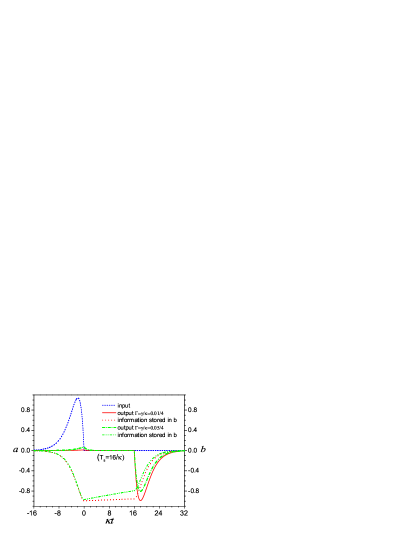
Figure 6: Atomic-coupled cavity input (dashed blue line), and output amplitudes with $\gamma/\kappa=0.01/4$ (solid black line), $\gamma/\kappa=0.05/4$ (dash-dotted green line) for the zero detuning strategy $\Delta=0$. Corresponding dashed thin lines represent the information $b(t)$ stored in the atom. Here $C\simeq 100$ and $T_{s}=16/\kappa$, and the critically damped case applies.

The coupling $g(t)$ is given as

$$g(t) = g\,\quad[t<0]$$

$$g(t) = 0\,\,\,[0<t<T]$$

$$g(t) = g\,\quad[t>T]\,.$$ (82)

Using $\kappa_{\pm}=(\kappa\pm\gamma)/2$ due to $\Delta=0$, we obtain the relation between the operators $a(0),$ $b(0)$ and $a_{0}^{in}$:

$$a(0) = \sqrt{2\kappa}\sqrt{2(\kappa\gamma+g^{2})(\kappa+\gamma)}\int_{-\infty}^{0}e^{2\kappa_{+}\tau}\frac{-i}{m}$$ (83)

$$\times[ch(m(\tau)+\frac{\kappa_{-}sh(m\tau)}{2m}]sh(m\tau)a_{0}^{in}d\tau+noise$$

$$= \frac{\sqrt{\kappa}\gamma i}{\sqrt{(\kappa\gamma+g^{2})(\kappa+\gamma)}}a_{0}^{in}+noise\,,$$

$$b(0) = \sqrt{2\kappa}\sqrt{2(\kappa\gamma+g^{2})(\kappa+\gamma)}\frac{g}{m^{2}}$$ (84)

$$\times\int e^{2\kappa_{+}\tau}sh^{2}(m\tau)a_{0}^{in}d\tau+noise$$

$$= \frac{\sqrt{\kappa}g}{\sqrt{(\kappa\gamma+g^{2})(\kappa+\gamma)}}a_{0}^{in}+noise\,.$$

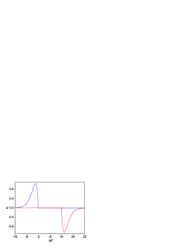
Figure 7: Atomic-coupled cavity input (dashed blue line) and output (solid red line) amplitudes in the zero detuning $\Delta=0$ case with $\kappa=4$, $g=2$, $\gamma=0.01$, $T_{S}=4.0$, using direct numerical integration. Input mode shape is mode matched to the critical cavity decay.

After a time $T$, the time reversed $g(t)$ retrieves the cavity mode into the output mode $u_{0}^{out*}(t)=u_{0}^{in}(T-t)$, which is the time reverse of $u_{0}^{in}(t)$. The optimal function for the cavity output pulse is thus

$$a_{0}^{out} = \int_{T}^{\infty}u_{0}^{out*}(t)a_{out}(t)dt\,,$$

$$a_{out}(t) = \sqrt{2\kappa}a(t)-A_{v}^{in}(t)\,.$$ (85)

After calculating the relevant integrals, but omitting the explicit form of the “noise” terms, we have

$$a_{0}^{out} = \frac{\sqrt{\kappa}\gamma ia(T)+\sqrt{\kappa}gb(T)}{\sqrt{(\kappa\gamma+g^{2})(\kappa+\gamma)}}+noise$$ (86)

$$= \frac{-\kappa\gamma^{2}e^{-\kappa T}+\kappa g^{2}e^{-(\gamma+i\Delta)T}}{(\kappa\gamma+g^{2})(\kappa+\gamma)}a_{0}^{in}+noise$$

$$= \sqrt{\eta_{M}}a_{0}^{in}+\sqrt{1-\eta_{M}}a_{0}^{r}$$

which reduces to (25) where $a_{0}^{r}$ is the reservoir mode arising from the “noise” term, and $\sqrt{\eta_{M}}$ is the overall memory efficiency given by

$$\sqrt{\eta_{M}} = \frac{\kappa g^{2}e^{-\gamma T}-\kappa\gamma^{2}e^{-\kappa T}}{(\kappa\gamma+g^{2})(\kappa+\gamma)}$$ (87)

$$= \frac{Ce^{-\gamma T}}{(1+C)(1+\Gamma)}-\frac{\Gamma e^{-\kappa T}}{(1+C)(1+\Gamma)}.$$

Here, we introduce the cooperativity parameter $C=g^{2}/\kappa\gamma$ and $\Gamma=\gamma/\kappa$. This result agrees with that obtained previously theory cavity , in the limit of $C\gg\Gamma$, or $\kappa T$ large enough so that the second term is negligible. The optimal case is to ensure large $C\gg\Gamma$, $C\gg 1$, large $\kappa$ compared to $\gamma$, so $\Gamma$ is small. It is still necessary however to ensure that the storage time is small enough so that $\gamma T\ll 1$. However, $T$ can be many cavity lifetimes, $\kappa T\gg 1$. We note we do not want $\Gamma=1$ because critical damping would require zero $g$. If $m=0$ , so that $g=\kappa_{-}=(\kappa-\gamma)/2$, we obtain the critically damped case for which the desired input temporal mode function is

$$u_{0}^{in}(t)=\frac{-i\kappa_{+}}{\sqrt{2}}\sqrt{\kappa_{+}}e^{\kappa_{+}t/2}t\,.$$ (88)

Fig. 6 shows the typical input-output relation for various loss ratios during the storage time of duration $T$. For the same cavity damping $\kappa$, different rates of optical coherence decay will result in different memory efficiencies. For $\gamma=0.01,$ $\sqrt{\eta_{M}}=0.95$, while for $\gamma=0.05,$ $\sqrt{\eta_{M}}=0.80.$ We can use the ratio of the integral of envelope between $a_{0}^{out}$ and $a_{0}^{in}$ $[\int u_{0}^{out*}(t)a_{out}(t)dt/\int_{-\infty}^{0}u_{0}^{in*}(t)a_{in}(t)dt$] to check the value of $\sqrt{\eta_{M}}$. If $\gamma$ is larger, the atomic lifetime is shorter, which means the information stored in the medium decays more quickly (shown by thin dashed green curve), resulting in a reduced efficiency.

In summary, with an appropriate selection of mode-matched filters, we are still able to retrieve the input signal with high efficiency, provided $\Gamma\ll 1$. The results are confirmed by numerical integration of the coupled cavity-oscillator equations, as shown in Fig. 7. This numerical method thus serves as a way to explore more sophisticated nonlinear models of the atomic medium.

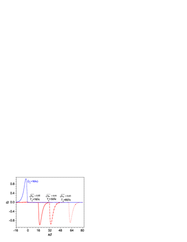
Figure 8: Atomic-coupled cavity input (dashed blue line) and output (solid black line) amplitudes with $\gamma/\kappa=0.01/4$ and different storage time $T_{S}=4$, 8, 15. Input mode shape is mode matched to the critical cavity decay. $\kappa=4$, $g=2$.

To analyse the effectiveness of the memory as a quantum memory, we must calculate the mean fidelity. Here we consider, for definiteness, the simplest encoding strategy with coherent states. Other strategies - for example using an arbitrary state with photon number bounds - will generally have different thresholds, as explained in Section (II).

For the case of $\overline{n}=1$, any retrieval with $\sqrt{\eta_{M}}>0.293$ can be claimed to be a “quantum memory”. For $\overline{n}>20$ (Fig. 3), the curve of required average fidelity as a function of mean number of photons is very flat and close to the classical boundary nature05136 , which is why low photon numbers are preferable in experiments on quantum memory, if high fidelity is required. At $\overline{n}=20$ we need a much higher retrieval efficiency of $\sqrt{\eta_{M}}>0.80$ to ensure the device is a true quantum memory.

A long storage time $T$ is consistent with high memory fidelity $\bar{F}$ (Fig. 8), provided we optimise for high efficiency using mode matching, and provided the atomic losses are not significant over the storage time ($\gamma T\ll 1$). For an input signal duration $\tau_{p}=4$, with residual loss $\gamma=0.01$, we get a retrieval efficiency $\sqrt{\eta_{M}}=0.95$, $0.91$, $0.85$ for the storage times $T=4$, $8$, $15$ respectively. The average fidelities are $\overline{F}=0.95,$ $0.86$, $0.69$, respectively, all of them larger than the classical bound $\overline{F}=0.51$ required for a quantum memory at $\overline{n}=20$. Thus, for these parameters, with input states giving $\overline{n}=20$, we are able to predict the existence of a quantum memory, with both high fidelity and relatively long memory lifetime. At lower photon numbers of $\overline{n}\sim 1$, a much higher loss is possible before loss of quantum memory.

V.2 Time-varying detuning

In experiments using two-level atoms one may control the coupling by with a time-varying detuning $\Delta(t)$ hetet . During writing and reading the atoms are strongly coupled to the field to allow transfer of the quantum state. During storage, the coupling is decreased by using a greatly increased detuning, controllable via a magnetic field or a Stark shift. To model this case, we employ a time-varying detuning with $\Delta_{L}\gg\kappa,$$\gamma$:

$$\begin{array}[]{ccccc}\Delta(t)&=&&0&[t<0]\\ \Delta(t)&=&&\Delta_{L}&[0<t<T/2]\\ \Delta(t)&=&-&\Delta_{L}&[T/2<t<T]\\ \Delta(t)&=&&0&[t>T]\,.\end{array}$$ (89)

Here, the storage period is divided into two parts with opposite detunings in order to ensure the phase is the same between signal and output field. In the writing and reading periods, choosing critical damping $g=\kappa_{-}=(\kappa-\gamma)/2$ expressed in real terms with detuning $\Delta=0,$ we will have the same input mode $u_{0}^{in}(t)$ as above. The overall memory efficiency in this case is

$$\sqrt{\eta_{M}} = \frac{4\kappa(g^{2}e^{-\gamma T}-\gamma^{2}e^{-\kappa T})}{(\kappa+\gamma)^{3}}\,,$$ (90)

which is the same form as Eq. (87) for the critically damped case.

The atomic-coupled cavity input and output amplitudes with $\gamma=0.01,$ $\Delta_{L}=27\pi$ is shown in Fig. 9. The dashed black line represents the desired output mode shape matched to the critical cavity decay.

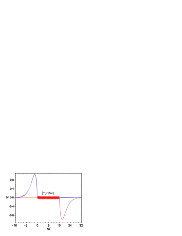
Figure 9: Atomic-coupled cavity input (dashed blue line) and output amplitudes with $\gamma/\kappa=0.01/4$ (solid red line). Input mode shape is mode matched to the critical cavity decay. $\kappa=4$, $g=(\kappa-\gamma)/2$, $T_{S}=4.0$,$\Delta_{L}=27\pi$.

VI Summary

We consider a general protocol for a dynamical quantum memory, using a cavity-oscillator model. Our definition of an acceptable quantum memory is based on two elementary criteria. To qualify as a quantum device, it must have a fidelity over a given set of input states that is better than any classical measure and regenerate strategy. To qualify as a memory it must be able store the input state over a time-scale longer than the input signal duration.

We analyse fidelity measures using both a coherent state input and an arbitrary quantum superposition input. Our general conclusion is that an optimal memory performance of a quantum memory is obtained through mode-matching the input pulse shape to a specific input mode of the memory device.

Three models of quantum memory are considered, of increasing complexity. All the models possess a time-reversal symmetry, so that output modes are obtained through a time-reversal of the input modes. First, to introduce the importance of temporally mode-matching the input pulse to the cavity mode, we consider a simple Q-switched cavity. This is sensitive to cavity losses during the storage period, which are difficult to eliminate.

Next, we introduce a model of a linearly coupled atomic memory, including losses, but with step-function modulation of the coupling. Provided a suitably modified asymmetric temporal mode is used, the effects of cavity loss are suppressed for long atomic lifetimes, and it is possible to largely decouple the input quantum mode from the lossy intracavity field mode. We show that there is an optimal coupling strength which generates a mode-matched input and output pulse. Finally, we consider a model in which the detuning is modulated in time, and show that this has a similar behaviour to the modulated coupling protocol.

With tailored input and output mode shapes, this type of quantum memory device promises to give both relatively long memory lifetimes and high memory quality.

- (1) L. M. Duan, M. D. Lukin, J. I. Cirac and P. Zoller, Nature, 414, 413 (2001).
- (2) Z.W. Barber, C.W. Hoyt, C.W. Oates, L. Hollberg, A.V. Taichenachev and V. I. Yudin, Phys. Rev. Lett. 96, 083002 (2006); A.V. Taichenachev, V. I. Yudin, C.W. Oates, C.W. Hoyt, Z.W. Barber, and L. Hollberg, Phys. Rev. Lett. 96, 083001 (2006).
- (3) Jun Ye, H. J. Kimble, Hidetoshi Katori, Science 320, 1734 (2008).
- (4) B. Julsgaard, J. Sherson, J. I. Cirac, J. Fiurek and E. S. Polzik, Nature 432, 482 (2004).
- (5) D. F. Phillips, A. Fleischhauer, A. Mair, R. L. Walsworth, and M. D. Lukin, Phys. Rev. Lett. 86, 783 (2001).
- (6) T. Chaneliere, D. N. Matsukevich, S. D. Jenkins, S. Y. Lan, T. A. B. Kennedy, and A. Kuzmich, Nature (London) 438, 833 (2005).
- (7) M. D. Eisaman, A. Andre, F. Massou, M. Fleischhauer, A. S. Zibrov, and M. D. Lukin, Nature (London) 438, 837 (2005).
- (8) C. W. Chou, H. de Riedmatten, D. Felinto, S. V. Polyakov, S. J. van Enk, and H. J. Kimble, Nature (London) 438, 828 (2005).
- (9) J. Appel, E. Figueroa, D. Korystov, M. Lobino and A. I. Lvovsky, Phys. Rev. Lett. 100, 093602 (2008).
- (10) K. Honda, D. Akamatsu, M. Arikawa, Y. Yokoi, K. Akiba, S. Nagatsuka, T. Tanimura, A. Furusawa and M. Kozuma, Phys. Rev. Lett. 100, 093601 (2008).
- (11) M. Fleischhauer and M. D. Lukin, Phys. Rev. Lett. 84, 5094 (2000).
- (12) S. A. Moiseev and S. Kroll, Phys. Rev. Lett. 87, 173601 (2001).
- (13) G. Hetet, J. J. Longdell, A. L. Alexander, P. K. Lam, and M. J. Sellars, Phys. Rev. Lett. 100, 023601 (2008).
- (14) R. J. Schoelkopf and S. M. Girvin, Nature 451, 664 (2008).
- (15) J. Q. You and F. Nori, Phys. Today 58 , 42 (2005).
- (16) M. A. Castellanos-Beltran, K. D. Irwin, G. C. Hilton, L. R. Vale, and K. W. Lehnert, arXiv: 0806.0659.
- (17) J D Thompson, B M Zwickl, A M Jayich, Florian Marquardt, S M Girvin, J G E Harris, Nature 452, 72 (2008).
- (18) S. Bose, K. Jacobs, P. L. Knight, Phys. Rev. A 59, 3204 (1999); S. Mancini, D. Vitali, V. Giovannetti, P. Tombesi, Eur. Phys. J. D 22, 417 (2003); W. Marshall, C. Simon, R. Penrose, D. Bouwmeester, Phys. Rev. Lett. 91, 130401 (2003).
- (19) Hiroyuki Yamada, Katsuji Yamamoto, Opt. Comm. 274, 384 (2007).
- (20) M. A. Sillanpää, J. I. Park, and R. W. Simmonds, Nature 449, 438 (2007).
- (21) Shi-Biao Zheng, Guang-Can Guo, Phys. Lett. A 232, 171 (1997).
- (22) P. Grangier, Science 281, 56 (1998).
- (23) P. Grangier, G. Reymond, and Schlosser, Fortschr. Phys. 48, 859 (2000).
- (24) P. Marek and R. Filip, Phys. Rev. A 70, 022305 (2004).
- (25) Tatjana Wilk, Simon C. Webster, Axel Kuhn, Gerhard Rempe, Science 317, 488 (2007).
- (26) C. Di Fidio, W. Vogel, M. Khanbekyan and D.-G. Welsch, Phys. Rev. A 77, 043822 (2008).
- (27) Jonathan Simon, Haruka Tanji, James K. Thompson and Vladan Vuletic, Phys. Rev. Lett. 98, 183601 (2007).
- (28) M. D. Lukin, S. F. Yelin and M. Fleischhauer, Phys. Rev. Lett. 84, 4232 (2000).
- (29) A. S. Parkins and H. J. Kimble, J. Opt. B: Quantum Semiclass. Opt. 1, 496 (2000).
- (30) Alexey V. Gorshkov, Axel Andre, Mikhail D. Lukin, and Anders S. Sorensen, Phys. Rev. A 76, 033804 (2007).
- (31) A. Dantan, A. Bramati, and M. Pinard, Phys. Rev. A 71, 043801 (2005).
- (32) A. Dantan, J. Cviklinski, M. Pinard and P. Grangier, Phys. Rev. A , 032338 (2006).
- (33) V. B. Braginsky, S. E. Strigin, and S. P. Vyatchanin, Phys. Lett. A 287, 331 (2001); T. J. Kippenberg, H. Rokhsari, T. Carmon, A. Scherer, and K. J. Vahala, Phys. Rev. Lett. 95, 033901 (2005).
- (34) Florian Marquardt, Joe P. Chen, A. A. Clerk, and S. M. Girvin, Phys Rev Letts 99, 093902 (2007).
- (35) H. Haken Laser Theory, Springer-Verlag, Berlin (1984).
- (36) P. D. Drummond, I.E.E.E J. Quant. Electron. QE-17, 301 (1981).
- (37) P. D. Drummond and M. G. Raymer, Phys. Rev. A 44, 2072 (1991).
- (38) M. J. Collett and C. W. Gardiner, Phys. Rev. A 30 , 1386 (1984).
- (39) C. W. Gardiner and M. J. Collett, Phys. Rev. A 31, 3761 (1985).
- (40) A. F. Pace, M. J. Collett and D. F. Walls, Phys. Rev. A 47, 3173 (1993).
- (41) P. D. Drummond, Phys. Rev. A42, 6845-6857 (1990).
- (42) A. Furusawa, J. L. Sørensen, S. L. Braunstein, C. A. Fuchs, H. J. Kimble, and E. S. Polzik, Science 282, 5389, 706 (1998).
- (43) K. Hammerer, M. M. Wolf, E. S. Polzik and J. I. Cirac, Phys. Rev. Lett. 94, 150503 (2005).
- (44) S. L. Braunstein, C. A. Fuchs, and H. J. Kimble, J. Mod. Opt. 47, 267 (2000).
- (45) G. Adesso and G. Chiribella, Phys. Rev. Lett. 100, 170503 (2008).
- (46) S. Massar and S. Popescu, Phys. Rev. Lett. 74, 1259 (1995). R. Derka, V. Buzek and A. K. Ekert, Phys. Rev. Lett. 80, 1571 (1998), V. Buzek and M. Hillery, Phys. Rev. Lett. 81, 5003 (1998).
- (47) R. J. Glauber, Phys. Rev. 130, 2529 (1963); E. C. G. Sudarshan, Phys. Rev. Lett. 10, 277 (1963).
- (48) P. D. Drummond and C. W. Gardiner, J. Phys. A13, 2353-2368 (1980).
- (49) J. F. Sherson, H. Krauter, R. K. Olsson, B. Julsgaard, K. Hammerer, I. Cirac, and E. S. Polzik, Nature (London) 443, 557 (2006).